| Issue |
A&A
Volume 520, September-October 2010
|
|
|---|---|---|
| Article Number | A89 | |
| Number of page(s) | 12 | |
| Section | Stellar structure and evolution | |
| DOI | https://doi.org/10.1051/0004-6361/200913796 | |
| Published online | 08 October 2010 | |
Physical elements of the eclipsing binary
 Orionis
![[*]](/icons/foot_motif.png) ,,
,,
P. Mayer1 - P. Harmanec1 - M. Wolf1 - H. Bozic2 - M. Slechta3
1 - Astronomical Institute of the Charles University,
Faculty of Mathematics and Physics,
V Holesovickách 2, 180 00 Praha 8, Czech
Republic
2 - Hvar Observatory, Faculty of Geodesy, Zagreb University, Kaciceva
26, 10000 Zagreb, Croatia
3 - Astronomical Institute, Academy of Sciences of the Czech Republic,
251 65 Ondrejov, Czech Republic
Received 3 December 2009 / Accepted 1 June 2010
Abstract
For years, ![]() Orionis
was considered a normal binary with an O9.5 II
primary exhibiting apsidal-line advance. However, radial-velocity
curves of both binary components have been derived from the IUE and
optical spectra using the cross-correlation technique, and surprisingly
low masses of 11.2 and 5.6
Orionis
was considered a normal binary with an O9.5 II
primary exhibiting apsidal-line advance. However, radial-velocity
curves of both binary components have been derived from the IUE and
optical spectra using the cross-correlation technique, and surprisingly
low masses of 11.2 and 5.6 ![]() were found. We obtained new spectra in the red spectral region and new UBV
photometry. Using all published photometry and radial velocities, we
deduced more accurate orbital and apsidal line periods. The main result
of this paper is to show that the observed line spectra of
were found. We obtained new spectra in the red spectral region and new UBV
photometry. Using all published photometry and radial velocities, we
deduced more accurate orbital and apsidal line periods. The main result
of this paper is to show that the observed line spectra of ![]() Orionis
are composed of the lines of the O9.5 II primary and a
similarly hot tertiary, while the lines of a cooler B-type secondary
are too faint to be detected in the available spectra. The character of
the light curve (low-amplitude partial eclipses and a non-negligible
scatter of the data) does not allow for a unique light-curve solution.
Nevertheless, we show that the assumption of normal primary-component
mass and radius corresponding to the O9.5 II classification
(25
Orionis
are composed of the lines of the O9.5 II primary and a
similarly hot tertiary, while the lines of a cooler B-type secondary
are too faint to be detected in the available spectra. The character of
the light curve (low-amplitude partial eclipses and a non-negligible
scatter of the data) does not allow for a unique light-curve solution.
Nevertheless, we show that the assumption of normal primary-component
mass and radius corresponding to the O9.5 II classification
(25 ![]() ,
16-17
,
16-17 ![]() )
leads to consistent parameters for the system.
)
leads to consistent parameters for the system.
Key words: binaries: eclipsing - stars:
early-type - stars: fundamental parameters - stars: individual: ![]() Ori
Ori
1 Introduction
The star ![]() Orionis
A (HR 1852, HD 36486, HIP 25930) is one of
the brightest
eclipsing binaries on the sky. It has an orbital period of
5
Orionis
A (HR 1852, HD 36486, HIP 25930) is one of
the brightest
eclipsing binaries on the sky. It has an orbital period of
5
![]() 732, the primary star is of
spectral type O 9.5 II (Walborn 1972),
visual magnitude of the system is 2
732, the primary star is of
spectral type O 9.5 II (Walborn 1972),
visual magnitude of the system is 2
![]() 20 at maximum, and depths of
minima
are 0
20 at maximum, and depths of
minima
are 0
![]() 11 and 0
11 and 0
![]() 07 for the primary and
secondary, respectively. The
eclipsing binary is a member of the multiple visual star
ADS 4134.
Besides the somewhat faint and distant components B
and C, there is a close
component Ab discovered by Heintz (1980) and
confirmed by speckle interferometry (Mason et al. 1999) and by Hipparcos
satellite
(Perryman & ESA 1997). The last source gives the
separation between Aa and Ab as 0
07 for the primary and
secondary, respectively. The
eclipsing binary is a member of the multiple visual star
ADS 4134.
Besides the somewhat faint and distant components B
and C, there is a close
component Ab discovered by Heintz (1980) and
confirmed by speckle interferometry (Mason et al. 1999) and by Hipparcos
satellite
(Perryman & ESA 1997). The last source gives the
separation between Aa and Ab as 0
![]() 267
and their magnitude
difference 1
267
and their magnitude
difference 1
![]() 35 (probably the average
difference during the orbit).
Horch et al. (2001)
give the magnitude difference 1
35 (probably the average
difference during the orbit).
Horch et al. (2001)
give the magnitude difference 1
![]() 59. A preliminary
astrometric orbit with a period of 201 years has been
published by Mason et al. (2009). They give
the magnitude difference 1
59. A preliminary
astrometric orbit with a period of 201 years has been
published by Mason et al. (2009). They give
the magnitude difference 1
![]() 4, which will be used
hereafter.
4, which will be used
hereafter.
The binary has been studied many times. The first four radial
velocities (RV) were published by Vogel & Scheiner (1892), and the RV
variability was discovered by Deslandres (1900a, b) and confirmed
by Campbell (1901).
Deslandres (1900a)
analysed 11 Meudon RVs and concluded that ![]() Orionis
is a spectroscopic binary with a period of 1
Orionis
is a spectroscopic binary with a period of 1
![]() 92 and a highly eccentric
orbit. Hartmann (1904)
obtained and analysed Potsdam RVs, including the remeasured early RVs
of Vogel & Scheiner (1892).
He found that the correct orbital period, also reconciling Deslandres'
and Campbell's RVs
is 5
92 and a highly eccentric
orbit. Hartmann (1904)
obtained and analysed Potsdam RVs, including the remeasured early RVs
of Vogel & Scheiner (1892).
He found that the correct orbital period, also reconciling Deslandres'
and Campbell's RVs
is 5
![]() 7325
7325 ![]() 0
0
![]() 0002.
A number of studies followed. These were summarized by Harvey
et al.
(1987) who
derived new RVs from the International Ultraviolet
Explorer (IUE) SWP spectra. After analysing published and new
RVs
they got a sidereal period of 5
0002.
A number of studies followed. These were summarized by Harvey
et al.
(1987) who
derived new RVs from the International Ultraviolet
Explorer (IUE) SWP spectra. After analysing published and new
RVs
they got a sidereal period of 5
![]() 732403, the eccentricity e=0.087,
and the period of the apsidal-line rotation of
732403, the eccentricity e=0.087,
and the period of the apsidal-line rotation of ![]() years. Also
the value of
years. Also
the value of ![]() km s-1
appeared well established.
Luyten et al. (1939)
gave the mass ratio 2.6, and with it, Koch & Hrivnak (1981) obtained
quite acceptable masses: 23 and 9
km s-1
appeared well established.
Luyten et al. (1939)
gave the mass ratio 2.6, and with it, Koch & Hrivnak (1981) obtained
quite acceptable masses: 23 and 9 ![]() .
.
Owing to its brightness, this binary could be a welcome source
of precise
physical properties of early-type stars; but the presence of the visual
component and the low depths of minima (and probably also some
intrinsic
variability) make the exploitation of observations rather difficult.
In a recent study, Harvin et al. (2002; hereafter
H02) published new values of masses and other parameters of the binary
components
(also discussed by Harvin & Gies 2002). They
found
quite surprising masses for the system components: M1=11.2
and
M2=5.6 ![]() .
These values followed from the radial-velocity (RV hereafter) curve
semiamplitudes obtained using 60 high-dispersion IUE spectra
and also a set of ground-based spectra, which consisted of
6 KPNO and 14 Mount Stromlo Observatory spectra, all
with resolution
.
These values followed from the radial-velocity (RV hereafter) curve
semiamplitudes obtained using 60 high-dispersion IUE spectra
and also a set of ground-based spectra, which consisted of
6 KPNO and 14 Mount Stromlo Observatory spectra, all
with resolution
![]() to 32 000 and an S/N of
200 to 300 pixel-1. To obtain RVs, H02
used the cross-correlation function (CCF). The inclination of the orbit
was found from the solution of the light curve obtained by Hipparcos.
to 32 000 and an S/N of
200 to 300 pixel-1. To obtain RVs, H02
used the cross-correlation function (CCF). The inclination of the orbit
was found from the solution of the light curve obtained by Hipparcos.
One would expect a considerably higher mass for the primary
component,
perhaps not as high as expected by H02 (26-30 ![]() ), but
certainly above 20
), but
certainly above 20 ![]() ;
e.g., in Schmidt-Kaler (1982)
the
value 22
;
e.g., in Schmidt-Kaler (1982)
the
value 22 ![]() can be interpolated for the given spectral type and
luminosity. Heap et al. (2006)
give such a value for the O 9.7 III star. The low
masses of components obtained by H02 are difficult to explain; since
the orbit is eccentric, it seems probable that
there was no strong interaction between the primary and secondary
in the previous history of the binary, and both components should have
been evolving as single stars.
can be interpolated for the given spectral type and
luminosity. Heap et al. (2006)
give such a value for the O 9.7 III star. The low
masses of components obtained by H02 are difficult to explain; since
the orbit is eccentric, it seems probable that
there was no strong interaction between the primary and secondary
in the previous history of the binary, and both components should have
been evolving as single stars.
In Sect. 5, it is shown that, although the primary
component is evolved
to a radius well over MS, it is safely inside its Roche lobe. We
compared the ![]() Orionis
spectra with synthetic spectra (CMFGEN - Hillier &
Miller 1998,
OSTAR - Lanz & Hubeny 2003,
BSTAR - Lanz & Hubeny 2007)
and found no indications that the components (namely, the primary one)
possess any abnormalities as might be the case for very low masses. The
IR excess noted by H02 is only modest. Therefore, some doubts about the
H02 results are natural.
Orionis
spectra with synthetic spectra (CMFGEN - Hillier &
Miller 1998,
OSTAR - Lanz & Hubeny 2003,
BSTAR - Lanz & Hubeny 2007)
and found no indications that the components (namely, the primary one)
possess any abnormalities as might be the case for very low masses. The
IR excess noted by H02 is only modest. Therefore, some doubts about the
H02 results are natural.
In several cases, unexpected masses of certain binaries were
ultimately
explained by the presence of the spectral lines of a third body.
Since ![]() Orionis is also a
triple system, the strange masses found by H02
can perhaps be also due to inappropriate treatment of the
contribution of the third body to the observed line profiles.
Orionis is also a
triple system, the strange masses found by H02
can perhaps be also due to inappropriate treatment of the
contribution of the third body to the observed line profiles.
The problem can lie in the application of the CCF method to
the IUE
spectra with their relatively low S/N.
It is surprising - as
H02 themselves admit - that no trace of the visual companion was found
in the IUE spectra. This companion should perhaps contribute more light
in UV than in visual (using 1
![]() 4 mag difference,
4 mag difference,
![]() ;
L1+L2+L3=1)
since there are reasons to expect
that its temperature is higher than the temperature of the primary, see
Sect. 6. Very probably, the irregular and ill-defined CCF as
shown in
Fig. 3
of H02 is the reason; the line of the third body that is very
wide (see Sect. 4) might go unnoticed there.
;
L1+L2+L3=1)
since there are reasons to expect
that its temperature is higher than the temperature of the primary, see
Sect. 6. Very probably, the irregular and ill-defined CCF as
shown in
Fig. 3
of H02 is the reason; the line of the third body that is very
wide (see Sect. 4) might go unnoticed there.
That the third line was not recognized in the IUE spectra was the reason the secondary line was ``found''. The complicated process used by H02 to separate this line from the CCF profile does not appear as convincing. The results can be explained equally well as the effect of the third line. The red and blue extensions of this wide line might be misinterpreted as ``secondary lines''. This is particularly notable in the lower part of Fig. 4 of H02, where the dark areas have the form of straight lines and not of a sine curve. We show in Sect. 4 that the true lines of the secondary are much weaker than those found by H02.
In the H02 study, ![]() Orionis
is compared with
Orionis
is compared with ![]() Cir
and LZ Cep, where
masses lower than expected were found as well. In both these binaries,
the mass deviation is only modest, and the mass determination is not
without problems, especially due to the uncertain inclinations. Since
Cir
and LZ Cep, where
masses lower than expected were found as well. In both these binaries,
the mass deviation is only modest, and the mass determination is not
without problems, especially due to the uncertain inclinations. Since
![]() Cir
is also a triple star and was analysed with the CCF
(Penny et al. 2001),
determination of its component masses could be affected in a similar
way to the case of
Cir
is also a triple star and was analysed with the CCF
(Penny et al. 2001),
determination of its component masses could be affected in a similar
way to the case of ![]() Ori.
On the other hand,
LZ Cep is a semi-detached binary (Harries
et al. 1998),
therefore its component masses should differ from normal ones.
Ori.
On the other hand,
LZ Cep is a semi-detached binary (Harries
et al. 1998),
therefore its component masses should differ from normal ones.
2 Observational material used
We compiled all published RVs with known times of observations, accumulated since 1888, and derived HJDs for them. We also reduced 20 Reticon and 204 CCD spectrograms obtained in the coudé spectrograph of the Ondrejov 2.0-m reflector between 1993 and 2010. Details on the reduction and measurements of the new spectra and compilation of published RVs can be found in Appendix A. All individual RVs with HJDs are provided for future use in electronic-only Table 1.
We obtained new ![]() observations at Hvar and also compiled available
observations with known dates of observations. A detailed account
of these data, their reduction and homogenization is in
Appendix B. For the convenience of future investigators, we
publish
both the new and all the available photoelectric observations
homogenized by us in electronic-only Table 2. The orbital
phase plots for all numerous enough data sets, which were
obtained in the visual spectral region are shown in Fig. 1.
One can see that neither light curve is ideal for the determination of
the basic physical elements of the binary. To read Fig. 1
properly, please note that only Stebbins, Hipparcos,
and Hvar
observations are shown as individual observations, all others being
either normal points or means of several consecutive observations. At
Hvar,
observations at Hvar and also compiled available
observations with known dates of observations. A detailed account
of these data, their reduction and homogenization is in
Appendix B. For the convenience of future investigators, we
publish
both the new and all the available photoelectric observations
homogenized by us in electronic-only Table 2. The orbital
phase plots for all numerous enough data sets, which were
obtained in the visual spectral region are shown in Fig. 1.
One can see that neither light curve is ideal for the determination of
the basic physical elements of the binary. To read Fig. 1
properly, please note that only Stebbins, Hipparcos,
and Hvar
observations are shown as individual observations, all others being
either normal points or means of several consecutive observations. At
Hvar, ![]() Orionis can only be
observed at air masses of 1.4 and
higher which contributes to the scatter (also seen in the
observations of the check star 33 Ori). In spite of these
shortcomings,
the changing position of the secondary minimum due to apsidal motion is
clearly seen.
Orionis can only be
observed at air masses of 1.4 and
higher which contributes to the scatter (also seen in the
observations of the check star 33 Ori). In spite of these
shortcomings,
the changing position of the secondary minimum due to apsidal motion is
clearly seen.
![\begin{figure}
\par\includegraphics[width=4.95cm,clip]{13796f01.eps}\par\include...
...{13796f06.eps}\par\includegraphics[width=4.95cm,clip]{13796f07.eps}
\end{figure}](/articles/aa/full_html/2010/12/aa13796-09/img36.png)
|
Figure 1:
Phase plots for individual homogenized data sets obtained in the visual
region. Ephemeris used:
Primary min.
|
| Open with DEXTER | |
3 Improved ephemeris including the apsidal advance
The collected and new photometric and spectroscopic material allows deriving the improved ephemeris for the system. We used two computer programs: FOTEL (Hadrava 1990, 2004a) and PHOEBE (Prsa & Zwitter 2005a,b, 2006) which is a development of the well-known program WD of Wilson and Devinney (1971), further developed by Wilson (see, e.g. Wilson 2007).
We proceeded in the following way:
- 1.
- We used all published RVs, complemented by our measurements of red Ondrejov spectrograms, to derive a solution with FOTEL. The period and the rate of apsidal advance were included in the solution and individual systemic velocities were derived for individual datasets of Table 1. Using the rms errors of individual datasets from this first solution, we weighted the datasets by outer weights inversely proportional to the squares of these rms errors and derived the final FOTEL RV solution. This is given in Table 3.
- 2.
- Using PHOEBE, we derived an independent solution for all light curves, also allowing for the convergency of the period and the rate of apsidal advance. This solution is also given in Table 3 under the name PHOEBE LC. It shows that there is a fairly good mutual agreement between the elements from spectroscopy and photometry.
- 3.
- To derive the final ephemeris to be used, we therefore
imported
all RV measurements of the primary into PHOEBE.
Note, however, that
the available versions of the WD program (and PHOEBE
) can only
treat one single file of the radial velocities for each component. This
is not suitable since individual RV datasets of
 Orionis
have obviously
different systemic velocities (cf., e.g., Fig. 10 in H02),
probably
because of different zero points of different observers. The
expected variation in the systemic velocity as the binary orbits the
common centre of gravity with the distant tertiary does not agree with
the observed changes. (The probable time of the periastron is in the
middle of the last century, and in that time the velocity change should
be
largest, but the observed velocity is nearly constant in that time.)
For
PHOEBE, we therefore used RVs with the
individual systemic velocities
(as derived in the final FOTEL solution)
subtracted. This means that
one has to fix a zero systemic velocity in PHOEBE.
This solution,
which gives the final ephemeris, is the solution denoted PHOEBE
LC&RV in
Table 3.
Orionis
have obviously
different systemic velocities (cf., e.g., Fig. 10 in H02),
probably
because of different zero points of different observers. The
expected variation in the systemic velocity as the binary orbits the
common centre of gravity with the distant tertiary does not agree with
the observed changes. (The probable time of the periastron is in the
middle of the last century, and in that time the velocity change should
be
largest, but the observed velocity is nearly constant in that time.)
For
PHOEBE, we therefore used RVs with the
individual systemic velocities
(as derived in the final FOTEL solution)
subtracted. This means that
one has to fix a zero systemic velocity in PHOEBE.
This solution,
which gives the final ephemeris, is the solution denoted PHOEBE
LC&RV in
Table 3.
Table 3: Trial orbital and light-curve solutions aimed at determination of improved ephemeris for the binary.
4 Towards true RV curves
Besides the Balmer and He I 6678 Å
lines, He II lines are also
present
in the spectra of ![]() Ori:
namely, the 6683 Å line is clearly visible at
the red wing of the He I 6678 Å
line. The C III 5695 Å
line is
in emission, as it is common among stars of
O 9.5 spectral type and
luminosity classes III and higher.
Ori:
namely, the 6683 Å line is clearly visible at
the red wing of the He I 6678 Å
line. The C III 5695 Å
line is
in emission, as it is common among stars of
O 9.5 spectral type and
luminosity classes III and higher.
H02 concludes that three of their He I 6678 Å
profiles were affected by some
emission. Although our line profiles differ in their widths and depths,
we found no evidence of emission in them. The differences are at the
level of about ![]() 6%,
but changes of EWs are small. Variable
emission/absorption is however present in H
6%,
but changes of EWs are small. Variable
emission/absorption is however present in H![]() ,
as already discussed by
Singh (1982).
This is why we restrict this study to
analysis of He lines.
,
as already discussed by
Singh (1982).
This is why we restrict this study to
analysis of He lines.
When analysing the He I 6678 Å line, H02 applied the CCF method, as in the case of the IUE spectra. However, they are silent about the line of the tertiary, although its effect on the primary and secondary lines might be strong. Once again, we conclude the wings of the third line are probably responsible for the residuals in their Fig. 7.
To provide quantitative support for our alternative interpretation, we used two independent techniques:
- modelling the He I 6678 Å line profiles with Gaussians profiles properly shifted in RV;
- analysing them with the disentangling program KOREL (Hadrava 1995, 1997, 2004b).
![\begin{figure}
\par\includegraphics[angle=-90,width=8.8cm,clip]{13796f08.eps}
\vspace*{-2.5mm}
\end{figure}](/articles/aa/full_html/2010/12/aa13796-09/img44.png)
|
Figure 2: Upper panel: an example of the observed profile (full line) with Gaussians for the He I and He II lines of the primary (dashed lines) and a broad, rotational profile for the third component (dotted line). Central panel: profiles of the observed spectra (He II feature subtracted); among them there is the space for the third line. Bottom panel: average profiles of quadratures and conjunction spectra (He II feature subtracted). The rotational profile of the third body is included. |
| Open with DEXTER | |
4.1 Modelling the profiles with two Gaussians
The spectra taken during an interval shorter than 1 h were
co-added
for the purpose of this analysis. Our iterative procedure is
illustrated
in a series of diagrams that follows. The upper panel of Fig. 2
provides an example of the ![]() 6678
& 6683 Å blend.
The observed profile is fitted with two Gaussians for the primary
contribution, the deeper for the He I 6678 Å
line, the shallower for the He II 6683 Å
line. The He II 6683 Å
Gaussian has FWHM
= 6.5 Å and depth 0.015 of the
continuum; with such values, one can fit all observed profiles (more
accurate fitting see below). The FWHM of the
primary Gaussian varies
from 3.7 to 4.6 Å, the depth from 0.099 to 0.128. For the
profile
shown in the upper panel, FWHM
= 4.12 Å, depth 0.114, RV = 117.9 km s-1.
In the case of a very positive velocity, the red wing of the
profile is only formed by the primary He II
line, without any
contribution from the tertiary or secondary.
6678
& 6683 Å blend.
The observed profile is fitted with two Gaussians for the primary
contribution, the deeper for the He I 6678 Å
line, the shallower for the He II 6683 Å
line. The He II 6683 Å
Gaussian has FWHM
= 6.5 Å and depth 0.015 of the
continuum; with such values, one can fit all observed profiles (more
accurate fitting see below). The FWHM of the
primary Gaussian varies
from 3.7 to 4.6 Å, the depth from 0.099 to 0.128. For the
profile
shown in the upper panel, FWHM
= 4.12 Å, depth 0.114, RV = 117.9 km s-1.
In the case of a very positive velocity, the red wing of the
profile is only formed by the primary He II
line, without any
contribution from the tertiary or secondary.
To compare the profiles observed at various phases, we subtracted the He II 6683 Å line from them. These corrected profiles, with the exception of those having a low S/N, are plotted in the central panel of Fig. 2. Clearly, the third-line contribution (TC) has to be common to all profiles; i.e., TC might fill the free space between the plotted profiles. No other process can explain the upper parts of the profiles except the presence of another component.
The space is fitted well by a rotational profile from the
OSTAR database
(Lanz & Hubeny 2003)
for ![]() K,
K,
![]() ,
,
![]() km s-1.
The profile is shifted in RV to
V=+25 km s-1
and reduced to 0.31 of its intensity.
km s-1.
The profile is shifted in RV to
V=+25 km s-1
and reduced to 0.31 of its intensity.
The large width of TC agrees with the results of H02, but describes the contribution more accurately. It also excludes the possibility, mentioned by H02, that the third component itself could be a binary; the wings of the observed profiles at identical phases would have to vary, which is not the case.
It would, of course, be desirable to also identify the
spectral line of
the secondary. This line should be visible in the profiles taken at
quadratures and invisible in profiles taken near conjunctions.
Therefore, we formed three groups of observed profiles and calculated
their averages: from spectra with RVs over 105 km s-1,
below -85 km s-1 and
between +3 and +25 km s-1.
These averaged profiles are shown in
the bottom panel of Fig. 2.
The space for the secondary line is
only between the quadrature profiles and the conjunction profile. But
nothing is visible between these profiles in quadrature with a positive
primary RV, and there is only a small space in the other quadrature.
Certainly no large contribution from the secondary, comparable to what
is advocated by H02, is acceptable (the expected positions of the
secondary
lines in quadratures are shown for K2=186,
![]() km s-1).
km s-1).
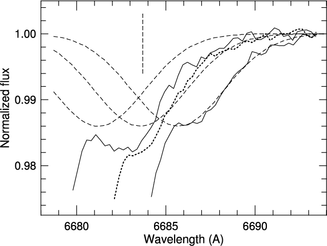
To understand the absorption in the red wings we subtracted
the He I 6678 Å profile
of the third body from the observed profiles. This profile is
independent of the phase, but the He II 6683 Å
profile might be phase dependent
from the strong dependence of this line on temperature and gravity (see
e.g. Lanz & Hubeny 2003). Figure 3 shows the profiles
averaged
for several phase intervals. Clearly, the profile for the quadrature
with a positive primary RV agrees with the Gaussian profile we used in
the former step. But an additional absorption is present
in the quadrature with the negative primary RV. Its maximum is at
6683 Å, so this could be the He I 6678 Å
line of the secondary with an RV of ![]() 220 km s-1.
However, a similar additional absorption, with an identical wavelength,
is also seen in the conjunction profile; in any case, it would be
strange if the secondary line was visible in only one quadrature.
220 km s-1.
However, a similar additional absorption, with an identical wavelength,
is also seen in the conjunction profile; in any case, it would be
strange if the secondary line was visible in only one quadrature.
|
Figure 3:
The red wings of the observed He I 6678 Å
profiles after subtracting the line profile of the third body.
From the left:
the profile at quadrature with the most negative primary RV (solid
line), the profiles at conjunctions (dotted line), and the profile at
quadrature with the most positive primary RV (full line). The dashed
lines represent the corresponding contributions from the primary He
II 6683 Å
profile. The vertical dashed line is at |
| Open with DEXTER | |
|
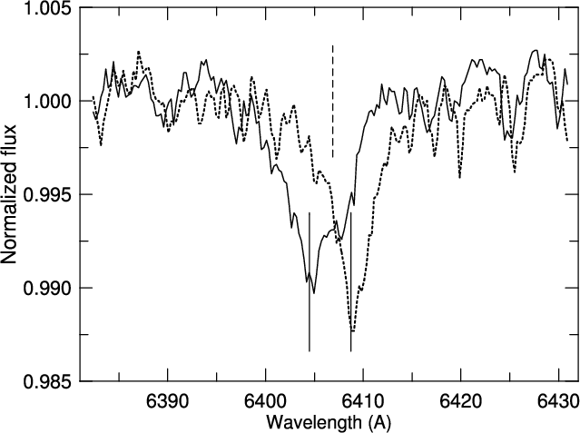
Figure 4:
Profile of the He II 6406 Å
line in both quadratures. Full vertical lines denote the expected line
positions corresponding to K1=106.3 km s-1,
|
| Open with DEXTER | |
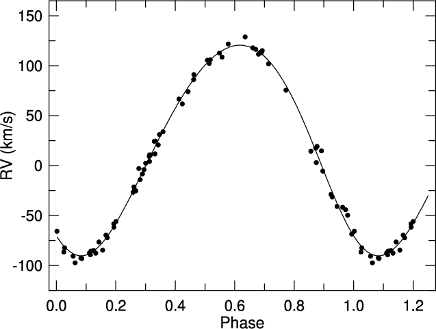
|
Figure 5:
Radial velocity curve of |
| Open with DEXTER | |
A definitive answer can be given by the He II 6406.4 Å
line, which is present in our spectra as a weak feature. This line is
also strongly dependent on ![]() and
and ![]() .
Its profiles in both quadratures
(obtained as sums of a dozen of observed spectra) presented in
Fig. 4
display similar behaviour to He II 6683 Å:
there is an additional
absorption near zero velocity in the profile at the quadrature with the
negative primary RV. As no such absorption is present at the opposite
quadrature, this absorption cannot originate in the third body or in
the secondary. However, to study it in more detail, more spectra of
He II lines would be needed.
.
Its profiles in both quadratures
(obtained as sums of a dozen of observed spectra) presented in
Fig. 4
display similar behaviour to He II 6683 Å:
there is an additional
absorption near zero velocity in the profile at the quadrature with the
negative primary RV. As no such absorption is present at the opposite
quadrature, this absorption cannot originate in the third body or in
the secondary. However, to study it in more detail, more spectra of
He II lines would be needed.
The measured Gaussian RVs of the primary are plotted in
Fig. 5
and the corresponding orbital solution presented in Table 4;
the rms per 1 RV observation is 4.1 km s-1.
The orbit was calculated again using the program FOTEL.
The anomalistic period and the rate of
periastron advance were kept fixed at values of 5
![]() 732821 and
0.00422 degrees per day. As could be expected, and as is known
from other cases (see e.g.
LY Aur, Popper 1982),
when a TC is taken into account, the resulting semi-amplitude of the
primary RV curve increases. In the previous
studies of
732821 and
0.00422 degrees per day. As could be expected, and as is known
from other cases (see e.g.
LY Aur, Popper 1982),
when a TC is taken into account, the resulting semi-amplitude of the
primary RV curve increases. In the previous
studies of ![]() Orionis
- including H02 - the effect of the third line on
the primary RVs was not considered; therefore, our K1
is larger than
for all already published RVs.
Orionis
- including H02 - the effect of the third line on
the primary RVs was not considered; therefore, our K1
is larger than
for all already published RVs.
4.2 Spectral disentangling
We used the program KOREL![]() developed by Hadrava (1995,
1997, 2004b) to the
spectral
disentangling. Preparation of data for the program KOREL
deserves a few
comments. The Ondrejov spectra have dispersion of
17.2 Å
and are recorded with a wavelength step of 0.256 Å, which
translates
to an RV resolution of about 12 km s-1.
For investigation of the
neighbourhood of the He I 6678 Å
and He II 6406 Å, we
oversampled the
spectra, rebinning them with steps of 2.2 and 2.0 km s-1,
respectively.
The rebinning was carried out with the help of the HEC35D
program
written by PH
developed by Hadrava (1995,
1997, 2004b) to the
spectral
disentangling. Preparation of data for the program KOREL
deserves a few
comments. The Ondrejov spectra have dispersion of
17.2 Å
and are recorded with a wavelength step of 0.256 Å, which
translates
to an RV resolution of about 12 km s-1.
For investigation of the
neighbourhood of the He I 6678 Å
and He II 6406 Å, we
oversampled the
spectra, rebinning them with steps of 2.2 and 2.0 km s-1,
respectively.
The rebinning was carried out with the help of the HEC35D
program
written by PH![]() ,
which derives consecutive discrete wavelengths via
,
which derives consecutive discrete wavelengths via
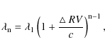
where
Table 4: The orbital solution with FOTEL based on the Gaussian RVs of the primary.
To take the variable quality of individual spectra into
account, we
measured their S/N in the
line-free region 6630-6650 Å, and
assigned each spectrum a weight according to formula
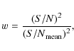
where
We briefly recall that KOREL uses the observed spectra and derives both the orbital elements and the mean individual line profiles of the two binary components. Considering that some spectra were obtained during the eclipses and that the object also exhibits obvious physical line-strength variations, we allowed for variable strengths of the spectral lines in individual spectra during the solutions - cf. Hadrava (1997).
Our experience with KOREL is that the
result is sensitive to the choice
of starting values of the elements and initial values of the simplex
steps. This is understandable since the sum of squares of residuals
using all data points of individual spectra is a very complicated one,
and
it is easy to end up in a local minimum. This has been nicely
illustrated in an excellent study of DW Car by Southworth
& Clausen
(2007) - see
their Fig. 3.
There is also another problem to complicate the task
of finding the optimal elements. If - as is obviously the case for
![]() Orionis - the
spectral lines of the secondary component are much fainter
than those of the primary, their effect on the resulting sum of squares
is very small. As a consequence, solutions for a wide range of mass
ratios would appear as comparably good ones.
Orionis - the
spectral lines of the secondary component are much fainter
than those of the primary, their effect on the resulting sum of squares
is very small. As a consequence, solutions for a wide range of mass
ratios would appear as comparably good ones.
Before mapping the sum of residuals vs. trial values of the
semiamplitude
of the primary, we derived trial solutions, using the value of K1estimated
from the Gaussian fits and adopting the astrometric solution
of Mason et al. (2009)
for the orbit of the tertiary. We investigated
two useful spectral regions: the neighbourhood of the He I 6678 Å
line and
a close neighbourhood of the He II 6406 Å
line. In these trial
solutions, we allowed disentangling of both spectral regions into three
stellar components. We obtained straight lines at continuum
for both
the disentangled secondary in the two regions and the tertiary
in the He II 6406 Å line
region. In other words, no
lines of the secondary and the He 6406 line of the tertiary
could be
detected above the detection treshold of some 0.003 of the
continuum level.
For that reason, we did the final parameter space mapping for the
primary
and tertiary only for He I 6678 Å
![]() ,
and for the primary and the telluric spectrum
for the neighbourhood of the He II 6406 Å
line.
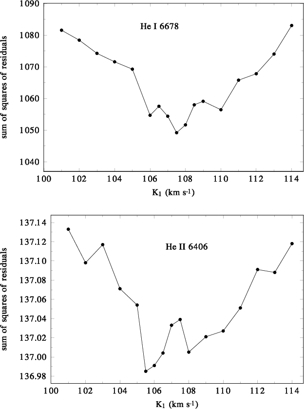
The plot of the sum of squares of residuals as a function of the
semi-amplitude K1 is shown
in Fig. 6,
separately for the
He I 6678 Å and He II 6406 Å
line.
One can see that the variation is not quite smooth but that it
clearly identifies the most probable semi-amplitude of the
primary near some 107 km s-1,
in good agreement with the result
based on the Gaussian fits.
,
and for the primary and the telluric spectrum
for the neighbourhood of the He II 6406 Å
line.
The plot of the sum of squares of residuals as a function of the
semi-amplitude K1 is shown
in Fig. 6,
separately for the
He I 6678 Å and He II 6406 Å
line.
One can see that the variation is not quite smooth but that it
clearly identifies the most probable semi-amplitude of the
primary near some 107 km s-1,
in good agreement with the result
based on the Gaussian fits.
We then derived a number of trial solutions where we only kept
the
anomalistic period (5
![]() 732821), apsidal advance
(0.00422 degrees per day) and eccentricity fixed, and starting
with K1 near
107 km s-1. The final KOREL
solutions for both lines, giving the
smallest sums of residuals, are in Table 5. Renormalizing the
continua of disentangled spectra according to the light-curve solution
(see the next section), we obtained the final line profiles shown
in Fig. 7.
732821), apsidal advance
(0.00422 degrees per day) and eccentricity fixed, and starting
with K1 near
107 km s-1. The final KOREL
solutions for both lines, giving the
smallest sums of residuals, are in Table 5. Renormalizing the
continua of disentangled spectra according to the light-curve solution
(see the next section), we obtained the final line profiles shown
in Fig. 7.
|
Figure 6: The sum of squares of residuals of exploratory KOREL solutions as a function of the semiamplitude of the primary K1 for the He II 6678 Å and He II 6406 Å lines. See the text for details. |
| Open with DEXTER | |
Table 5: KOREL disentangling orbital solutions for the spectral regions near the He I 6678 Å line, and near the He II 6406 Å line.
![\begin{figure}
\par\includegraphics[width=9cm,clip]{13796f14.eps}\par\includegraphics[width=9cm,clip]{13796f15.eps}
\end{figure}](/articles/aa/full_html/2010/12/aa13796-09/img64.png)
|
Figure 7: The line profiles disentangled by KOREL and normalized to their individual continua according to the light-curve solutions ( L1 = 0.755, L3=0.216). Upper panel: the He I 6678 Å and He II 6683 Å line profiles of the tertiary and primary. Bottom panel: the telluric spectrum and the He II 6406 Å line profile of the primary. In both panels, the spectra were shifted in flux for clarity, and there are very different flux scales in the two panels. |
| Open with DEXTER | |
5 Light-curve solution
Keeping the orbital period, the rate of apsidal advance, and
eccentricity
fixed at the values from the last solution of Table 3,
we derived the final combined solution with PHOEBE,
using
all available photometry and the Gaussian RVs for the primary.
The ![]() of the primary was kept fixed at
30 000 K because it follows, e.g., from the
calibration by Martins et al.
(2005). We also assumed that the third light contributed 21.6% in all
passbands and used linear limb darkening coefficients.
The anomalistic period and the rate of periastron advance were kept
fixed at values of 5
of the primary was kept fixed at
30 000 K because it follows, e.g., from the
calibration by Martins et al.
(2005). We also assumed that the third light contributed 21.6% in all
passbands and used linear limb darkening coefficients.
The anomalistic period and the rate of periastron advance were kept
fixed at values of 5
![]() 732821 and
0.00422 degrees per day.
Since we were unable to find any spectral lines of the secondary,
we had to assume something. We decided to adopt a reasonable mass
of 25
732821 and
0.00422 degrees per day.
Since we were unable to find any spectral lines of the secondary,
we had to assume something. We decided to adopt a reasonable mass
of 25 ![]() for the primary.
for the primary.
The solution with a free convergency (solution I) of
all elements gave
results that did not agree with expectations - the primary radius was
too small. As a consequence, the absolute visual magnitude and
the resulting distance were small. Also the effective temperature
of the secondary T2 was
under 20 000 K, although temperature of
a young 10 ![]() star should be about 24 000 K. Therefore, we derived
other solutions with the effective temperature
of the secondary fixed at 24 000 K. In
solution II, we moreover fixed
the relative radius of the primary, while in solution III the
relative
radius of the secondary was fixed. During solutions,
we tuned the mass ratio q to fit the known mass
function f(m)=0.71and the
inclination as it followed from the solution. The mass ratio
was always between 0.38 and 0.42, i.e.,
star should be about 24 000 K. Therefore, we derived
other solutions with the effective temperature
of the secondary fixed at 24 000 K. In
solution II, we moreover fixed
the relative radius of the primary, while in solution III the
relative
radius of the secondary was fixed. During solutions,
we tuned the mass ratio q to fit the known mass
function f(m)=0.71and the
inclination as it followed from the solution. The mass ratio
was always between 0.38 and 0.42, i.e., ![]()
![]() .
Our results
are summarized in Table 6.
.
Our results
are summarized in Table 6.
In the latest (development) version of PHOEBE
that we are using, the convergency is governed by minimalization of a
cost function ![]() defined in the case of our datasets as
defined in the case of our datasets as
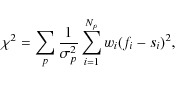
where index p denotes the individual photometric passbands,
Table 6: The final combined solution with PHOEBE, based on all photometric data sets and Gaussian RVs for the primary.
The cost function for both constrained solutions is naturally
a bit higher, but the comparison of the resulting model V
light curves with
the observed Hvar V light curve, presented in
Fig. 8,
shows that all these solutions fit the observed curve
within the limits of its scatter (all
photometry was used to obtain the solutions, but owing to apside
line advance, only observations from a limited time interval are
shown).
In other words, one must conclude
that a whole class of possible solutions is tolerable with the light
curves at hand. When H02 solved the Hipparcos
light curve, their result also was that a wide interval of solutions
is possible. Their radii of the primary 9 and 13 ![]() (obtained for a=34.5
(obtained for a=34.5 ![]() )
can be transformed for our
)
can be transformed for our ![]()
![]() to 11.5 and 16.6
to 11.5 and 16.6 ![]() .
In spite of including several times more numerous data, our results are
similar.
.
In spite of including several times more numerous data, our results are
similar.
Parameters that would follow from the system's membership in
the Orion complex are therefore allowed. The membership means that
the primary ![]() is about -
is about -
![]() .
The
.
The ![]() of the three-body system is then -
of the three-body system is then -
![]() and with the magnitude at maximum
and with the magnitude at maximum ![]() and interstellar absorption
and interstellar absorption ![]() the distance moduli is 8.0, comparable e.g. to the distance
413 pc of Trapezium
(Menten et al. 2007).
With the radius
the distance moduli is 8.0, comparable e.g. to the distance
413 pc of Trapezium
(Menten et al. 2007).
With the radius ![]() about 17
about 17 ![]() ,
the age of the primary is
,
the age of the primary is ![]() 5.5 My (Claret 2004);
the
secondary component is very probably a star of identical age. With the
mass
5.5 My (Claret 2004);
the
secondary component is very probably a star of identical age. With the
mass ![]() 10
10 ![]() ,
its radius should be about 4.3
,
its radius should be about 4.3 ![]() and temperature
24 000 K. Even with r1=0.38
the primary is well inside Roche lobe: its
volume equals about 57% of the Roche lobe volume as calculated using
the
formula by Eggleton (1983).
and temperature
24 000 K. Even with r1=0.38
the primary is well inside Roche lobe: its
volume equals about 57% of the Roche lobe volume as calculated using
the
formula by Eggleton (1983).
6 Discussion
In this paper, several arguments are given against detection of
secondary
absorption lines by H02 in ![]() Orionis
. It is mainly the unreliability
of the CCF results - very probably, CCFs obtained by H02 contain
information on the third line, not on the secondary. When
disentangling He I 6678 Å
line, H02 did not
Orionis
. It is mainly the unreliability
of the CCF results - very probably, CCFs obtained by H02 contain
information on the third line, not on the secondary. When
disentangling He I 6678 Å
line, H02 did not ![]() the secondary line, only
the secondary line, only
![]() it. Therefore, the component masses found by H02 cannot
be trusted.
it. Therefore, the component masses found by H02 cannot
be trusted.
![\begin{figure}
\par\includegraphics[width=8.8cm,clip]{13796f16.eps}
\end{figure}](/articles/aa/full_html/2010/12/aa13796-09/img86.png)
|
Figure 8: Hvar V measurements compared with PHOEBE solutions: I - full curve, II - short-dash curve, III - long-dash curve. |
| Open with DEXTER | |
According to the BSTAR spectra (Lanz & Hubeny 2007), theoretical
equivalent widths of the He I 6678 Å
line are ![]() 0.50 Å
in the
primary, as well as in the secondary component. Then the observed width
of the primary line should be 0.38 Å. (But the real observed
width
is 0.47 Å; such deviations are known for other high-luminosity
stars, too). Under assumptions of ``normality'' for both binary
components, the secondary is 26-times weaker in V,
and its observed
line should have EW = 0.015 Å.
If the components rotate synchronously, the secondary FWHM
is about 1.5 Å, therefore the line depth would
be 0.01 of the continuum. No such lines are visible in Figs. 2 (bottom) or 3; the limit for the
detection is several times smaller, i.e., the secondary He I 6678 Å
line is several times weaker than it should be.
0.50 Å
in the
primary, as well as in the secondary component. Then the observed width
of the primary line should be 0.38 Å. (But the real observed
width
is 0.47 Å; such deviations are known for other high-luminosity
stars, too). Under assumptions of ``normality'' for both binary
components, the secondary is 26-times weaker in V,
and its observed
line should have EW = 0.015 Å.
If the components rotate synchronously, the secondary FWHM
is about 1.5 Å, therefore the line depth would
be 0.01 of the continuum. No such lines are visible in Figs. 2 (bottom) or 3; the limit for the
detection is several times smaller, i.e., the secondary He I 6678 Å
line is several times weaker than it should be.
Therefore, instead of the problem of very low masses, we
are confronted with another problem - very small EW of the secondary
He I 6678 Å
line. We do not have any explanation; however, we can say that a very
similar situation was met by Popper (1993) in his discussion of the
spectra
of V1765 Cyg. This binary bears some similarity to ![]() Ori:
the spectral type
is B 0.5 Ib, the orbit is eccentric, and
Ori:
the spectral type
is B 0.5 Ib, the orbit is eccentric, and ![]() ;
the period is 13
;
the period is 13
![]() 4. Popper did not find the
secondary line
He I 5786 Å
and estimated that it is 35 times or more
weaker than the primary line, i.e. several times weaker than it should
be, the problem identical to the case of He I 6678 Å
in
4. Popper did not find the
secondary line
He I 5786 Å
and estimated that it is 35 times or more
weaker than the primary line, i.e. several times weaker than it should
be, the problem identical to the case of He I 6678 Å
in ![]() Ori.
Ori.
Because it is 1
![]() 4 fainter than the primary,
the third body should be of about O 9 IV type, with
4 fainter than the primary,
the third body should be of about O 9 IV type, with ![]() K.
In spite of this high temperature, the He II 6683 Å
and 6406 Å lines are not expected to be present as
both strongly depend on gravity. Naturally, it would be
helpful if a separated spectrum of the visual component could be
acquired, for example using adaptive optics.
K.
In spite of this high temperature, the He II 6683 Å
and 6406 Å lines are not expected to be present as
both strongly depend on gravity. Naturally, it would be
helpful if a separated spectrum of the visual component could be
acquired, for example using adaptive optics.
It is known that there are systems where the lines of their seconaries are invisible presumably due to circumstellar envelopes, but they possess longer periods (HD 187399, P=28 d, e=0.39) or circular orbits. In this connection, please note that the suggestion by H02 that the eccentricity might stem from the visual component is not acceptable, because the time scale of any such effect is about 1010 years, see Eggleton & Kiseleva-Eggleton (2001). Also the effect of the third body on the apside line rotation might only be small - according to Söderhjelm (1981), the apside line period would be 107 years if its only reason was the third body.
AcknowledgementsWe gratefully acknowledge the use of spectrograms of
References
- Campbell, W. W. 1901, PASP, 13, 162 [NASA ADS] [CrossRef] [Google Scholar]
- Campbell, W. W., & Moore, J. H. 1928, Publ. Lick Obs., 16, 74 [Google Scholar]
- Claret, A. 2004, A&A, 424, 919 [NASA ADS] [CrossRef] [EDP Sciences] [Google Scholar]
- Curtiss, R. H. 1915, Publ. Michigan, 1, 118 [NASA ADS] [Google Scholar]
- Deslandres, H. 1900a, Comptes Rendus, 130, 379 [Google Scholar]
- Deslandres, H. 1900b, Observatory, 23, 148 [NASA ADS] [Google Scholar]
- Deslandres, H. 1904, AN, 166, 33 [NASA ADS] [Google Scholar]
- Eggleton, P. P. 1983, ApJ, 268, 368 [NASA ADS] [CrossRef] [Google Scholar]
- Eggleton, P. P., & Kiseleva-Eggleton, L. 2001, ApJ, 562, 1012 [NASA ADS] [CrossRef] [Google Scholar]
- Hadrava, P. 1990, Contr. Astron. Obs. Skalnaté Pleso, 20, 23 [Google Scholar]
- Hadrava, P. 1995, A&AS, 114, 393 [NASA ADS] [Google Scholar]
- Hadrava, P. 1997, A&AS, 122, 581 [NASA ADS] [CrossRef] [EDP Sciences] [Google Scholar]
- Hadrava, P. 2004a, Publ. Astr. Inst. Acad. Sci. Czech Rep., 89, 1 [Google Scholar]
- Hadrava, P. 2004b, Publ. Astr. Inst. Acad. Sci. Czech Rep., 89, 15 [Google Scholar]
- Harmanec, P. 1998, A&A, 335, 173 [NASA ADS] [Google Scholar]
- Harmanec, P., & Bozic, H. 2001, A&A, 369, 1140 [NASA ADS] [CrossRef] [EDP Sciences] [Google Scholar]
- Harmanec, P., & Horn, J. 1998, J. Astron. Data, 4, file 5 [Google Scholar]
- Harmanec, P., Horn, J., & Juza, K. 1994, A&AS, 104, 121 [NASA ADS] [Google Scholar]
- Harries, T. J., Hilditch, R. W., & Hill, G. 1998, MNRAS, 295, 386 [NASA ADS] [CrossRef] [Google Scholar]
- Hartmann, J. 1904, ApJ, 19, 268 [Google Scholar]
- Harvey, A. S., Stickland, D. J., Howarth, I. D., & Zuiderwijk, E. J. 1987, Observatory, 107, 205 [NASA ADS] [Google Scholar]
- Harvin, J. A., & Gies, D. R. 2002, in Exotic Stars as Challenges to Evolution, ed. C. A. Tout, & W. van Hamme, ASP Conf. Ser., 279, 47 [Google Scholar]
- Harvin, J. A., Gies, D. R., Bagnuolo, W. G., Penny, L. R., & Thaller, M. 2002, ApJ, 565, 1216 [NASA ADS] [CrossRef] [Google Scholar]
- Heap, S. R., Lanz, T., & Hubeny, I. 2006, ApJ, 638, 409 [NASA ADS] [CrossRef] [Google Scholar]
- Heintz, W. D. 1980, ApJS, 44, 111 [NASA ADS] [CrossRef] [Google Scholar]
- Hill, G. 1982, Publ. Dominion Astrophys. Obs., 16, 67 [Google Scholar]
- Hillier, D. J., & Miller, D. L. 1998, ApJ, 496, 407 [NASA ADS] [CrossRef] [Google Scholar]
- Hnatek, A. 1921, AN, 213, 17 [NASA ADS] [Google Scholar]
- Holmgren, D. E., Hadrava, P., Harmanec, P., et al. 1999, A&A, 345, 855 [NASA ADS] [Google Scholar]
- Horch, E., Ninkov, Z., & Franz, O. G. 2001, AJ, 121, 1583 [NASA ADS] [CrossRef] [Google Scholar]
- Horn, J., Kubát, J., Harmanec, P., et al. 1996, A&A, 309, 521 [NASA ADS] [Google Scholar]
- Johnson, H. L., Iriarte, B., Mitchell, R. I., & Wisniewski, W. Z. 1966, CoLPL, 4, 99 [Google Scholar]
- Jordan, F. C. 1916, Publ. Allegheny Obs., 3, 125 [NASA ADS] [Google Scholar]
- Koch, R. H., & Hrivnak, B. J. 1981, ApJ, 248, 249 [NASA ADS] [CrossRef] [Google Scholar]
- Lanz, T., & Hubeny, I. 2003, ApJS, 146, 417 [NASA ADS] [CrossRef] [Google Scholar]
- Lanz, T., & Hubeny, I. 2007, ApJS, 169, 83 [CrossRef] [Google Scholar]
- Luyten, W. J., Struve, O., & Morgan, W. W. 1939, Publ. Yerkes Obs., 7, 256 [Google Scholar]
- Martins, F., Schaerer, D., & Hillier, D. J. 2005, A&A, 436, 1049 [NASA ADS] [CrossRef] [EDP Sciences] [Google Scholar]
- Mason, B. D., Martin, C., Hartkopf, W. I., Barry, D. J., Germain, M. E., et al. 1999, AJ, 117, 1890 [NASA ADS] [CrossRef] [Google Scholar]
- Mason, B. D., Hartkopf, W. I., Gies, D. R., Henry, T. J., & Helsel, J. W. 2009, AJ, 137, 3358 [NASA ADS] [CrossRef] [EDP Sciences] [Google Scholar]
- Menten, K. M., Reid, M. J., Forbrich, J., & Brunthaler, A. 2007, A&A, 474, 515 [NASA ADS] [CrossRef] [EDP Sciences] [Google Scholar]
- Miczaika, G. R. 1952, ZfA, 30, 299 [NASA ADS] [Google Scholar]
- Moultaka, J., Ilovaiski, S. A., Pruguiel, P., & Soubiran, C. 2004, PASP, 116, 693 [NASA ADS] [CrossRef] [Google Scholar]
- Natarajan, V., & Rajamohan, R. 1971, KodOB, 208, 219 [NASA ADS] [Google Scholar]
- Perryman, M. A. C., & ESA 1997, The Hipparcos & Tycho Catalogues, ESA SP-1200 [Google Scholar]
- Pismis, P., Haro, G., & Struve, O. 1950, ApJ, 111, 509 [NASA ADS] [CrossRef] [Google Scholar]
- Penny, L. R., Seyle, D., Gies, D. R., et al. 2001, ApJ, 575, 1050 [Google Scholar]
- Popper, D. M. 1982, ApJ, 262, 641 [NASA ADS] [CrossRef] [Google Scholar]
- Popper, D. M. 1953, PASP, 105, 721 [NASA ADS] [CrossRef] [Google Scholar]
- Prsa, A., & Zwitter, T. 2005a, ApJ, 628, 426 [NASA ADS] [CrossRef] [Google Scholar]
- Prsa, A., & Zwitter, T. 2005b, ESA SP-576, 611 [Google Scholar]
- Prsa, A., & Zwitter, T. 2006, Ap&SS, 304, 347 [NASA ADS] [CrossRef] [Google Scholar]
- Schmidt-Kaler, Th. 1982, in Landolt-Börnstein, 2b (Berlin: Springer), 453 [Google Scholar]
- Singh, M. 1982, Ap&SS, 87, 269 [NASA ADS] [CrossRef] [Google Scholar]
- Skoberla, P. 1935, ZfA, 11, 1 [NASA ADS] [Google Scholar]
- Skoda, P. 1996, in Astronomical Data Analysis Software and Systems V, ASP Conf. Ser., 101, 187 [Google Scholar]
- Söderhjelm, S. 1981, A&A, 42, 229 [Google Scholar]
- Southworth, J., & Clausen, J. V. 2007, A&A, 461, 1077 [NASA ADS] [CrossRef] [EDP Sciences] [Google Scholar]
- Stebbins, J. 1915, ApJ, 42, 133 [NASA ADS] [CrossRef] [Google Scholar]
- Stebbins, J. 1911, ApJ, 34, 105 [NASA ADS] [CrossRef] [Google Scholar]
- Storer, N. W. 1930, PASP, 42, 291 [NASA ADS] [CrossRef] [Google Scholar]
- Vogel, H. C., & Scheiner, J. 1892, Publ. Astrophys. Obs. Potsdam, 7, Part I, 100 [Google Scholar]
- Wilson, R. E. 2007, in IAU Symp. 240, ed. by W.I. Hartkopf, E.F. Guinan, & P. Harmanec (Cambridge Univ. Press), 188 [Google Scholar]
- Wilson, R. E., & Devinney, E. J. 1971, ApJ, 166, 605 [NASA ADS] [CrossRef] [Google Scholar]
- Walborn, N. L. 1972, AJ, 77, 312 [NASA ADS] [CrossRef] [Google Scholar]
- Worley, C. E. 1955, PASP, 67, 330 [NASA ADS] [CrossRef] [Google Scholar]
Online Material
Appendix A: Overview of available RV observations
Table A.1: Journal of available RV observations.
We reduced and measured two sets of electronic spectra
secured at the coudé focus of the 2-m reflector of the Ondrejov
Observatory which cover the red spectral region containing the H![]() and
He I 6678 Å lines. These
spectra have a linear dispersion of 17.2 Å mm-1and
a 2-pixel resolution of 12 700 (11-12 km s-1
per pixel).
and
He I 6678 Å lines. These
spectra have a linear dispersion of 17.2 Å mm-1and
a 2-pixel resolution of 12 700 (11-12 km s-1
per pixel).
- 1.
- In the period 1993-2000, 20 spectra were obtained with a Reticon 1872RF linear detector. They cover the wavelengths from 6305 to 6740 Å and have the S/N between 110 and 900.
- 2.
- A series of 204 spectrograms obtained with a
SITe-005
 CCD
detector secured between 2003 and 2010. They cover a slighly longer
wavelength region 6255-6765 Å and have S/N
between
200 and 880.
CCD
detector secured between 2003 and 2010. They cover a slighly longer
wavelength region 6255-6765 Å and have S/N
between
200 and 880.
The initial reductions of spectra were performed using the IRAF (Ondrejov CCD spectra and SPEFO (Ondrejov Reticon spectra) programs. All subsequent reductions and the RV measurements were carried out using the SPEFO reduction program written by the late Dr. J. Horn and then further developed by Dr. P. Skoda and by (now also late) Mr. J. Krpata (Horn et al. 1996; Skoda 1996). Note that SPEFO displays direct and reverse traces of the line profiles superimposed on the computer screen, and the user can slide them to achieve their exact ovelapping for the studied detail of the profile.
A.1. Radial-velocity data files
We carried out a critical compilation of all available RV measurements
from the literature with the known dates of observations.
In all cases where the original sources give the dates and times of
mid-exposures, we used the program HEC19 to
derive heliocentric Julian dates![]() .
The journal of all RVs used in this study is in Table A.1.
.
The journal of all RVs used in this study is in Table A.1.
When the number of measured lines N used to derive the mean RV was given in the original study, we applied internal weighting of individual RVs, assigning weights w = 0.1*N. The only exception are Vienna RVs based on the mean of 11-38 individual lines. Here we used a linear transformation from the interval (11, 38) to (0.5, 1.5).
Comments on some individual files follow:
- Spg. 1: Potsdam Four very first RVs of Orionis
were obtained
by Vogel & Scheiner (1892)
in 1888-1891 and showed no evidence of RV changes. They are based on RV
of H
 alone. When Deslandres (1900a)
discovered the RV variations, Prof. Vogel remeasured the old spectra at
the request of Dr. Hartmann. He found out that
the last two spectra do show significant RV changes. His revised RVs
are published in Hartmann's (1904)
paper and should be preferred over
the original measurements so are used by us.
alone. When Deslandres (1900a)
discovered the RV variations, Prof. Vogel remeasured the old spectra at
the request of Dr. Hartmann. He found out that
the last two spectra do show significant RV changes. His revised RVs
are published in Hartmann's (1904)
paper and should be preferred over
the original measurements so are used by us.
- Spg. 2: Meudon Deslandres (1900a,b) published his discovery RVs giving only the days of observations. Hartmann (1904) republished his RVs with estimated fractions of the days of observations, but later Deslandres (1904) published the actual mid-exposure times of his observations and these are used by us.
- Spg. 3: Lick Three RVs from 1900 Lick spectra taken with the Mills pectrograph were obtained and measured by Dr. Wright and published by Campbell (1901), again without accurate mid-exposure times. Hartmann (1904) also estimated the times of mid-exposures for these spectra but we use the actual mid-exposure times published by Campbell & Moore (1928), adopting also mean RV from two independent measurements of these spectra for this last publication.
- Spg. 6: Vienna Hnatek (1921) tabulated mid-exposure times in Central European Mean Time (G.M.T.+1 h) and used this time also for the fractions of his Julian days. We derived and used correct HJDs.
- Spg. 11: IUE Harvey et al. (1987) analysed the first 44 SWP spectra obtained by the IUE. Their RV measurements were relative and the RVs published in their Table 1 have the zero point artificially shifted in such a way as to give the systemic velocity of 20.4 km s-1, adopted from the study by Curtiss (1915). Harvin et al. (2002) later analysed the complete set of 60 IUE SWP spectra from the final IUE reduction. The derived RVs via cross-correlation, using the spectra of O 9.5V star AB Aur (HD 34078) as a template. Here we adopted their RVs.
- Spg. 14&15: Kitt Peak and Mt. Stromlo These RVs are solely based on the He I 6678 Å line and were also derived via cross-correlation by Harvin et al. (2002).
- Spg. 13&16: Ondrejov These RVs are also solely based on the He I 6678 Å line measured in SPEFO via comparison of direct and flipped line profile on the computer screen.
Appendix B: Photometry
After the discovery that ![]() Orionis
is an eclipsing variable by Stebbins
(1911, 1915), the binary
was measured by several authors: Storer (1930), Skoberla (1935; only times
of minima), Worley (1955,
who also published measurements by Storer), and Koch & Hrivnak (1981). Then
there is the photometry by Hipparcos.
Orionis
is an eclipsing variable by Stebbins
(1911, 1915), the binary
was measured by several authors: Storer (1930), Skoberla (1935; only times
of minima), Worley (1955,
who also published measurements by Storer), and Koch & Hrivnak (1981). Then
there is the photometry by Hipparcos.
Table B.1: Photometric data sets used.
Table B.2: Comparison and check stars used by various photometric observers.
We obtained new ![]() observations using the automated photoelectric
photometer attached to the 0.65-m reflector of the Hvar Observatory.
The data were transformed to the standard
observations using the automated photoelectric
photometer attached to the 0.65-m reflector of the Hvar Observatory.
The data were transformed to the standard ![]() system via
non-linear transformation (see Harmanec et al. 1994, for
details).
system via
non-linear transformation (see Harmanec et al. 1994, for
details).
The reductions were carried out with the latest
version 16.1 of the
HEC22 program (Harmanec & Horn 1998), which
permits extinction variations to be modelled in the course of the
night. To be able to also transform the old Stebbins (1915) photometry
to the V magnitude, we also observed his comparison
star ![]() Ori regularly during
the first season.
Ori regularly during
the first season.
The new observations were combined with several existing
photometric data
sets that we critically compiled from the literature. Basic information
about all data sets used is summarized in Table B.1.
Table B.2
summarizes the ![]() magnitudes of all comparison
stars used by different observers. Hvar mean all-sky magnitudes were
added to all magnitude differences
magnitudes of all comparison
stars used by different observers. Hvar mean all-sky magnitudes were
added to all magnitude differences ![]() Orionis
- comparison whenever these differences were known.
Orionis
- comparison whenever these differences were known.
A few comments on individual data sets follow:
- Stebbins (1915):
magnitude differences Orionis
-
 Ori,
secured with the Lick 12-inch refractor, were transformed
toJohnson V following Holmgren
et al. (1999)
and Harmanec & Bozic (2001).
The mean Hvar all-sky V magnitude of Ori,
1
Ori,
secured with the Lick 12-inch refractor, were transformed
toJohnson V following Holmgren
et al. (1999)
and Harmanec & Bozic (2001).
The mean Hvar all-sky V magnitude of Ori,
1
 695
695  0
019 was then added to the
transformed magnitude differences to get Stebbins' observations on the
standard Johnson V magnitude. Note,
however, that Ori
is a known variable star (see Fig. B.1), so these early
data must be treated with some caution.
0
019 was then added to the
transformed magnitude differences to get Stebbins' observations on the
standard Johnson V magnitude. Note,
however, that Ori
is a known variable star (see Fig. B.1), so these early
data must be treated with some caution.
- Storer (1930)
and Worley (1955):
Both these authors published their observations only in a graphical
form. Their observations were also secured with the
Lick 12-inch refractor, but no details about the photometer
used by Storer are known. Worley used an EMI 5659
photomultiplier and Corning filters 3385 and 5543, which very
closely match the B and V magnitudes
of the Johnson system. He obtained about 300 yellow and 250
blue observations and formed 112 running means of them. Storer
observed in the years 1926-1928 relative to
 Ori (V = 3
36) and only showed plots of
magnitude differences from several observed
eclipses. They range from about 0
1 to 0
2; apparently
the integral parts of the ordinate scale of his plot should be -1
instead zero. Worley (1955)
obtained Storer's individual observations but he published them along
with his own observations only in the form of a phase diagram, forming
the normal points from the original Storer's observations.
We therefore reconstructed these two sets of observations from his
plot and assigned them ``artificial'' Julian dates corresponding to the
mean times of observations of the respective data sets applying
the ephemeris that Worley probably used: HJD 2419068.20 + 5
Ori (V = 3
36) and only showed plots of
magnitude differences from several observed
eclipses. They range from about 0
1 to 0
2; apparently
the integral parts of the ordinate scale of his plot should be -1
instead zero. Worley (1955)
obtained Storer's individual observations but he published them along
with his own observations only in the form of a phase diagram, forming
the normal points from the original Storer's observations.
We therefore reconstructed these two sets of observations from his
plot and assigned them ``artificial'' Julian dates corresponding to the
mean times of observations of the respective data sets applying
the ephemeris that Worley probably used: HJD 2419068.20 + 5
 732476
  .
This ephemeris is still close to the present ephemeris
for the primary minimum. For the data by Storer (1930) and Worley
(1955), the
magnitude zero point is unknown, because Worley regrettably did not
mention which comparison star he used. Since the colours of the
comparison stars that were probably used are quite similar to those of Ori,
we treat these data as yellow magnitudes in the photometric solutions.
.
This ephemeris is still close to the present ephemeris
for the primary minimum. For the data by Storer (1930) and Worley
(1955), the
magnitude zero point is unknown, because Worley regrettably did not
mention which comparison star he used. Since the colours of the
comparison stars that were probably used are quite similar to those of Ori,
we treat these data as yellow magnitudes in the photometric solutions.
- Johnson et al. (1966): we derived
heliocentric Julian dates for these standard all-sky
 observations.
- Koch & Hrivnak (1981): these
authors obtained about 350 individual observations using a
photoelectric photometer with an RCA 4509 tube attached to the
0.38-m refractor of the Flower and Cook Observatory and
green and blue filters; however, they only published magnitude
differences
for 64 green and 62 blue normal points. We converted their JDs
to HJDs again. The primary comparison they
used,HD 36840 = HIP 26149, is a
seldom studied G5 star (
 = 6
25), and we found no way how
to transform their observations to the Johnson V
and B magnitudes. We therefore simply
added estimated green and blue magnitudes of HD 36840, 6
53, and 7
15 to the published magnitude
differences.
= 6
25), and we found no way how
to transform their observations to the Johnson V
and B magnitudes. We therefore simply
added estimated green and blue magnitudes of HD 36840, 6
53, and 7
15 to the published magnitude
differences.
- Perryman & ESA (1997) These Hipparcos
 observations
were transformed to the standard V magnitude
following Harmanec (1998)
and assuming the mean all-sky Hvar colour indices for Ori:
observations
were transformed to the standard V magnitude
following Harmanec (1998)
and assuming the mean all-sky Hvar colour indices for Ori:
 = -0
219, and
= -0
219, and  = -1
040 .
= -1
040 .
As a quality check, it is also useful to add a few comments on possible
light variations on other time scales.
All photometric observers of ![]() Orionis
have concluded that the object is exhibiting
cycle-to-cycle and, possibly also, hour-to-hour changes. The inspection
of Fig. 1
indeed reveals a rather large scatter in virtually
all visual light curves, although most of them are based on averaged
data. A word of caution is appropriate, however, because Stebbins' and
Storer's (if not also Worley's) observations were obtained using mildly
variable comparison stars. As Hvar observations show, the scatter
outside minima is comparable to what is observed for the check star and
can to some extent be attributed to the fact that the star could only
be observed at relatively high air masses.
Orionis
have concluded that the object is exhibiting
cycle-to-cycle and, possibly also, hour-to-hour changes. The inspection
of Fig. 1
indeed reveals a rather large scatter in virtually
all visual light curves, although most of them are based on averaged
data. A word of caution is appropriate, however, because Stebbins' and
Storer's (if not also Worley's) observations were obtained using mildly
variable comparison stars. As Hvar observations show, the scatter
outside minima is comparable to what is observed for the check star and
can to some extent be attributed to the fact that the star could only
be observed at relatively high air masses.
What can be suspected, however, is the different height of the maxima between the two eclipses, which might also vary secularly. Only more systematic observations from a good site can decide whether it is indeed so.
Footnotes
- ... Orionis
- Based on new spectral and photometric observations from the Hvar and Ondrejov observatories.
- ...
- Tables 1 and 2 are only available in electronic form at the CDS via anonymous ftp to cdsarc.u-strasbg.fr (130.79.128.5) or via http://cdsarc.u-strasbg.fr/viz-bin/qcat?J/A+A/520/A89
- ...
- Appendix A is only available in electronic form at http://www.aanda.org
- ... KOREL
- The freely distributed version from Dec. 2004.
- ... PH
- The program HEC35D with User's Manual is available to interested users at http://astro.troja.mff.cuni.cz/ftp/hec/HEC35
- ... edges
- This is necessary since KOREL requires that the number of the input data points is an integer multiple of 512.
- ... dates
- This program, which handles data in various forms, together with brief instructions on how to use it, is freely available on the anonymous ftp server at http://astro.troja.mff.cuni.cz/ftp/hec/HEC19.
- ...
- This value of the sidereal period is quoted by him and later also used by Koch & Hrivnak (1981), while the epoch had already been derived by Stebbins (1915) and used in subsequent studies.
All Tables
Table 3: Trial orbital and light-curve solutions aimed at determination of improved ephemeris for the binary.
Table 4: The orbital solution with FOTEL based on the Gaussian RVs of the primary.
Table 5: KOREL disentangling orbital solutions for the spectral regions near the He I 6678 Å line, and near the He II 6406 Å line.
Table 6: The final combined solution with PHOEBE, based on all photometric data sets and Gaussian RVs for the primary.
Table A.1: Journal of available RV observations.
Table B.1: Photometric data sets used.
Table B.2: Comparison and check stars used by various photometric observers.
All Figures
|
|
Figure 1:
Phase plots for individual homogenized data sets obtained in the visual
region. Ephemeris used:
Primary min.
|
| Open with DEXTER | |
| In the text | |
|
|
Figure 2: Upper panel: an example of the observed profile (full line) with Gaussians for the He I and He II lines of the primary (dashed lines) and a broad, rotational profile for the third component (dotted line). Central panel: profiles of the observed spectra (He II feature subtracted); among them there is the space for the third line. Bottom panel: average profiles of quadratures and conjunction spectra (He II feature subtracted). The rotational profile of the third body is included. |
| Open with DEXTER | |
| In the text | |
|
|
Figure 3:
The red wings of the observed He I 6678 Å
profiles after subtracting the line profile of the third body.
From the left:
the profile at quadrature with the most negative primary RV (solid
line), the profiles at conjunctions (dotted line), and the profile at
quadrature with the most positive primary RV (full line). The dashed
lines represent the corresponding contributions from the primary He
II 6683 Å
profile. The vertical dashed line is at |
| Open with DEXTER | |
| In the text | |
|
|
Figure 4:
Profile of the He II 6406 Å
line in both quadratures. Full vertical lines denote the expected line
positions corresponding to K1=106.3 km s-1,
|
| Open with DEXTER | |
| In the text | |
|
|
Figure 5:
Radial velocity curve of |
| Open with DEXTER | |
| In the text | |
|
|
Figure 6: The sum of squares of residuals of exploratory KOREL solutions as a function of the semiamplitude of the primary K1 for the He II 6678 Å and He II 6406 Å lines. See the text for details. |
| Open with DEXTER | |
| In the text | |
|
|
Figure 7: The line profiles disentangled by KOREL and normalized to their individual continua according to the light-curve solutions ( L1 = 0.755, L3=0.216). Upper panel: the He I 6678 Å and He II 6683 Å line profiles of the tertiary and primary. Bottom panel: the telluric spectrum and the He II 6406 Å line profile of the primary. In both panels, the spectra were shifted in flux for clarity, and there are very different flux scales in the two panels. |
| Open with DEXTER | |
| In the text | |
|
|
Figure 8: Hvar V measurements compared with PHOEBE solutions: I - full curve, II - short-dash curve, III - long-dash curve. |
| Open with DEXTER | |
| In the text | |
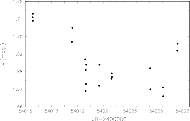
|
Figure
B.1:
A time plot of the Hvar V observations of |
| In the text | |
Copyright ESO 2010
Current usage metrics show cumulative count of Article Views (full-text article views including HTML views, PDF and ePub downloads, according to the available data) and Abstracts Views on Vision4Press platform.
Data correspond to usage on the plateform after 2015. The current usage metrics is available 48-96 hours after online publication and is updated daily on week days.
Initial download of the metrics may take a while.