| Issue |
A&A
Volume 520, September-October 2010
Pre-launch status of the Planck mission
|
|
|---|---|---|
| Article Number | A4 | |
| Number of page(s) | 21 | |
| Section | Astronomical instrumentation | |
| DOI | https://doi.org/10.1051/0004-6361/200912853 | |
| Published online | 15 September 2010 | |
Pre-launch status of the Planck mission
Planck pre-launch status: Design and description of the Low Frequency Instrument
M. Bersanelli1,2 - N. Mandolesi3 - R. C. Butler3 - A. Mennella1,2 - F. Villa3 - B. Aja4 - E. Artal4 - E. Artina5 - C. Baccigalupi6,15 - M. Balasini5 - G. Baldan5 - A. Banday7,32 - P. Bastia5 - P. Battaglia5 - T. Bernardino8 - E. Blackhurst9 - L. Boschini5 - C. Burigana3 - G. Cafagna5 - B. Cappellini1,2 - F. Cavaliere1 - F. Colombo5 - G. Crone10 - F. Cuttaia3 - O. D'Arcangelo11 - L. Danese6 - R. D. Davies9 - R. J. Davis9 - L. De Angelis12 - G. C. De Gasperis13 - L. De La Fuente4 - A. De Rosa3 - G. De Zotti14 - M. C. Falvella12 - F. Ferrari5 - R. Ferretti5 - L. Figini11 - S. Fogliani15 - C. Franceschet1 - E. Franceschi3 - T. Gaier16 - S. Garavaglia11 - F. Gomez17 - K. Gorski16 - A. Gregorio18 - P. Guzzi5 - J. M. Herreros17 - S. R. Hildebrandt17 - R. Hoyland17 - N. Hughes19 - M. Janssen16 - P. Jukkala19 - D. Kettle9 - V. H. Kilpiä19 - M. Laaninen20 - P. M. Lapolla5 - C. R. Lawrence16 - D. Lawson9 - J. P. Leahy9 - R. Leonardi21 - P. Leutenegger5 - S. Levin16 - P. B. Lilje22 - S. R. Lowe9 - P. M. Lubin21 - D. Maino1 - M. Malaspina3 - M. Maris15 - J. Marti-Canales10 - E. Martinez-Gonzalez8 - A. Mediavilla4 - P. Meinhold21 - M. Miccolis5 - G. Morgante3 - P. Natoli13 - R. Nesti23 - L. Pagan5 - C. Paine16 - B. Partridge24 - J. P. Pascual4 - F. Pasian15 - D. Pearson16 - M. Pecora5 - F. Perrotta15,6 - P. Platania11 - M. Pospieszalski25 - T. Poutanen26,27,28 - M. Prina16 - R. Rebolo17 - N. Roddis9 - J. A. Rubiño-Martin17 - M. J. Salmon8 - M. Sandri3 - M. Seiffert16 - R. Silvestri5 - A. Simonetto11 - P. Sjoman19 - G. F. Smoot29 - C. Sozzi11 - L. Stringhetti3 - E. Taddei5 - J. Tauber30 - L. Terenzi3 - M. Tomasi1 - J. Tuovinen31 - L. Valenziano3 - J. Varis31 - N. Vittorio13 - L. A. Wade16 - A. Wilkinson9 - F. Winder9 - A. Zacchei15 - A. Zonca1,2
1 - Università degli Studi di Milano, Dipartimento di Fisica, via
Celoria 16, 20133 Milano, Italy
2 - INAF - Istituto di Astrofisica Spaziale e Fisica Cosmica, via
Bassini 15, 20133 Milano, Italy
3 - INAF - Istituto di Astrofisica Spaziale e Fisica Cosmica, via P.
Gobetti, 101, 40129 Bologna, Italy
4 - Universidad de Cantabria, Departamento de Ingenieria de
Comunicaciones, Av. de Los Castros s/n, 39005 Santander, Spain
5 - Thales Alenia Space Italia S.p.A., S.S. Padana Superiore 290, 20090
Vimodrone, Milano, Italy
6 - SISSA/ISAS, Astrophysics Sector, Via Beirut 4, 34014 Trieste, Italy
7 - CESR, Centre d'Étude Spatiale des Rayonnements, 9 Av. du Colonel
Roche, BP 44346, 31028 Toulouse Cedex 4, France
8 - Instituto de Fisica de Cantabria, CSIC, Universidad de Cantabria,
Av. de los Castros s/n, 39005 Santander, Spain
9 - Jodrell Bank Centre for Astrophysics, Alan Turing Building, The
University of Manchester, Manchester, M13 9PL, UK
10 - Herschel/Planck Project,
Scientific Projects Dpt of ESA, Keplerlaan 1, 2200 AG, Noordwijk, The
Netherlands
11 - Istituto di Fisica del Plasma, CNR, via Cozzi 53, 20125 Milano,
Italy
12 - ASI, Agenzia Spaziale Italiana, viale Liegi, 26, 00198 Roma, Italy
13 - Dipartimento di Fisica, Università degli Studi di Roma Tor
Vergata, via della Ricerca Scientifica 1, 00133 Roma, Italy
14 - INAF - Osservatorio Astronomico di Padova, Vicolo
dell'Osservatorio 5, 35122 Padova, Italy
15 - INAF - Osservatorio Astronomico di Trieste, via Tiepolo, 11, 34143
Trieste, Italy
16 - Jet Propulsion Laboratory, California Institute of Technology,
4800 Oak Grove Drive, Pasadena, CA 91109, USA
17 - Instituto de Astrofisica de Canarias, C/ via Lactea s/n, 38200
La Laguna, Tenerife, Spain
18 - Dipartimento di Fisica, Università degli Studi di Trieste, via
A. Valerio 2, 34127 Trieste, Italy
19 - DA-Design Oy, Keskuskatu 29, 31600 Jokioinen, Finland
20 - Ylinen Electronics Oy, Teollisuustie 9A, 02700 Kauniainen, Finland
21 - Department of Physics, University of California, Santa Barbara,
CA 93106, USA
22 - Institute of Theoretical Astrophysics, University of Oslo, PO Box
1029 Blindern, 0315 Oslo, Norway
23 - INAF - Osservatorio Astrofisico di Arcetri, Largo Enrico Fermi 5,
50125 Firenze, Italy
24 - Haverford College, 370 Lancaster Avenue, Haverford, PA 19041, USA
25 - National Radio Astronomy Observatory, 520 Edgemont Rd,
Charlottesville, VA 22903-2475, USA
26 - University of Helsinki, Department of Physics, PO Box 64, 00014
Helsinki, Finland
27 - Helsinki Institute of Physics, University of Helsinki, PO Box 64,
00014, Finland
28 - Metsähovi Radio Observatory, Helsinki University of Technology,
Metsähovintie 114, 02540, Kylmälä, Finland
29 - Lawrence Berkeley National Laboratory, 1 Cyclotron Road, Berkeley,
CA 94720, USA
30 - European Space Agency (ESA), Astrophysics Division, Keplerlaan 1,
2201AZ Noordwijk, The Netherlands
31 - MilliLab, VTT Technical Research Centre of Finland, PO Box 1000,
02044 VTT, Finland
32 - MPA Max-Planck-Institut für Astrophysik, Karl-Schwarzschild-Str.
1, 85741 Garching, Germany
Received 8 July 2009 / Accepted 15 December 2009
Abstract
In this paper we present the Low Frequency Instrument (LFI), designed
and developed as part of the Planck space mission,
the ESA programme dedicated to precision imaging of the cosmic
microwave background (CMB). Planck-LFI will observe
the full sky in intensity and polarisation in three frequency bands
centred at 30, 44 and 70 GHz, while higher
frequencies (100-850 GHz) will be covered by the
HFI instrument. The LFI is an array of microwave radiometers
based on state-of-the-art indium phosphide cryogenic HEMT amplifiers
implemented in a differential system using blackbody loads as reference
signals. The front end is cooled to 20 K for optimal
sensitivity and the reference loads are cooled to 4 K to
minimise low-frequency noise. We provide an overview of
the LFI, discuss the leading scientific requirements, and
describe the design solutions adopted for the various hardware
subsystems. The main drivers of the radiometric, optical, and thermal
design are discussed, including the stringent requirements on
sensitivity, stability, and rejection of systematic effects. Further
details on the key instrument units and the results of ground
calibration are provided in a set of companion papers.
Key words: cosmic microwave background - cosmology: observations - space vehicles: instruments
1 Introduction
Observations of the cosmic microwave background (CMB) have played a
central role in the enormous progress of cosmology in the past few
decades. Technological developments in both coherent radio receivers
and bolometric detectors have supported an uninterrupted chain of
successful experiments, from the initial discovery (Penzias & Wilson 1965)
up to the present generation of precision measurements. Following COBE![]() and WMAP
and WMAP![]() , the Planck
, the Planck![]() satellite, launched on
14 May 2009, is the next-generation space
mission dedicated to CMB observations. The Planck
instruments are designed to extract all the cosmological information
encoded in the CMB temperature anisotropies with an accuracy
set by cosmic variance and astrophysical confusion limits, and to push
polarisation measurements well beyond previously reached results. Planck
will image the sky in nine frequency bands across the
CMB blackbody peak, leading to a full-sky map of the
CMB temperature fluctuations with
signal-to-noise >10 and angular
resolution <10'. The Planck
instruments and observing strategy were devised to reach an
unprecedented combination of angular
resolution (5' to 30'), sky
coverage (100%), spectral coverage (27-900 GHz),
sensitivity (
satellite, launched on
14 May 2009, is the next-generation space
mission dedicated to CMB observations. The Planck
instruments are designed to extract all the cosmological information
encoded in the CMB temperature anisotropies with an accuracy
set by cosmic variance and astrophysical confusion limits, and to push
polarisation measurements well beyond previously reached results. Planck
will image the sky in nine frequency bands across the
CMB blackbody peak, leading to a full-sky map of the
CMB temperature fluctuations with
signal-to-noise >10 and angular
resolution <10'. The Planck
instruments and observing strategy were devised to reach an
unprecedented combination of angular
resolution (5' to 30'), sky
coverage (100%), spectral coverage (27-900 GHz),
sensitivity (
![]()
![]() 2
2 ![]() 10-6),
calibration accuracy (
10-6),
calibration accuracy (![]() 0.5%),
and rejection of systematic effects (
0.5%),
and rejection of systematic effects (
![]() K per pixel)
(Tauber
et al. 2010a). In addition, all Planck
bands between 30 and 350 GHz are sensitive to linear
polarisation.
K per pixel)
(Tauber
et al. 2010a). In addition, all Planck
bands between 30 and 350 GHz are sensitive to linear
polarisation.
The imaging power of Planck is sized to extract the temperature power spectrum with high precision over the entire angular range dominated by primordial fluctuations. This will lead to accurate estimates of cosmological parameters that describe the geometry, dynamics, and matter-energy content of the universe. The Planck polarisation measurements are expected to deliver complementary information on cosmological parameters and to provide a unique probe of the thermal history of the universe in the early phase of structure formation. Planck will also test the inflationary paradigm with unprecedented sensitivity through studies of non-Gaussianity and of B-mode polarisation as a signature of primordial gravitational waves (Planck Collaboration 2005).
The wide frequency range of Planck is
required primarily to ensure accurate discrimination of foreground
emissions from the cosmological signal. However, the nine Planck
maps will also represent a rich data set for galactic and extragalactic
astrophysics. Up to now, no single technology can reach the
required performances in the entire Planck
frequency range. For this reason two complementary instruments are
integrated at the Planck focal plane exploiting
state-of-the-art radiometric and bolometric detectors in their best
windows of operation. The Low Frequency Instrument (LFI), described in
this paper, covers the 27-77 GHz range with a radiometer array
cooled to 20 K. The High Frequency Instrument (HFI)
will observe in six bands in the 90-900 GHz range with a
bolometer array cooled to 0.1 K (Lamarre et al. 2010).
The two instruments share the focal plane of a single telescope,
a shielded off-axis dual reflector Gregorian system with
1.5 ![]() 1.9 m
primary aperture (Tauber
et al. 2010b).
1.9 m
primary aperture (Tauber
et al. 2010b).
The design of the Planck satellite and
mission plan is largely driven by the extreme thermal requirements
imposed by the instruments. The cold payload enclosure
(<50 K passive cooling) needs to be thermally decoupled
from the warm (![]() 300 K)
service module while preserving high thermal stability. The optical
design, orbit, and scanning strategy are optimised to obtain the
required effective angular resolution, rejection of stray light, and
environmental stability. Planck has been injected
into a Lissajous orbit around the Sun-Earth L2 point,
at 1.5 million km from Earth. The scanning strategy
assumes, to first order, the spacecraft is spinning at
1 rpm with the spin axis aligned at 0
300 K)
service module while preserving high thermal stability. The optical
design, orbit, and scanning strategy are optimised to obtain the
required effective angular resolution, rejection of stray light, and
environmental stability. Planck has been injected
into a Lissajous orbit around the Sun-Earth L2 point,
at 1.5 million km from Earth. The scanning strategy
assumes, to first order, the spacecraft is spinning at
1 rpm with the spin axis aligned at 0![]() solar aspect angle.
The typical angle between the detectors' line of sight and the spin
axis is
solar aspect angle.
The typical angle between the detectors' line of sight and the spin
axis is ![]() .
It will be possible to redirect the spin axis within a cone
of
.
It will be possible to redirect the spin axis within a cone
of ![]() around the spacecraft-sun axis. The baseline mission allows for
15 months of routine scientific operations in L2,
a period in which the entire sky can be imaged twice by all
detectors. However, in anticipation of a possible extension of
the mission, spacecraft and instrument consumables allow an extension
by a factor of two
around the spacecraft-sun axis. The baseline mission allows for
15 months of routine scientific operations in L2,
a period in which the entire sky can be imaged twice by all
detectors. However, in anticipation of a possible extension of
the mission, spacecraft and instrument consumables allow an extension
by a factor of two![]() .
.
In this paper we present the design of the Planck-LFI and discuss its driving scientific requirements. We give an overview of the main subsystems, particularly those that are critical for scientific performance, while referring to a set of companion papers for more details. The LFI programme as a whole, including data processing and programming issues, is described in Mandolesi et al. (2010); the calibration plan and ground calibration results are discussed by Mennella et al. (2010) and Villa et al. (2010). The LFI optical design is presented in Sandri et al. (2010), while the expected polarisation performance is discussed in Leahy et al. (2010).
In Sect. 2.1 we discuss the main scientific requirements of LFI. We start from top-level guidelines such as frequency range, angular resolution, and sensitivity, and then move to more detailed requirements that were derived for the chosen design by assuming a moderate level of extrapolation of the technology available at the time of the design completion. In Sect. 3 we provide an overall description of LFI instrument configuration and discuss in detail the LFI differential radiometers and associated components. Section 4 is a description of the instrument system and subsystems, including optical, radiometric, and electronic units, while Sects. 4 to 7 describe the thermal, electrical, and optical interfaces.
2 Scientific requirements
In this section we discuss the main scientific requirements for the LFI. Here, and throughout this paper, we discuss instrument specifications, while measured on-ground performance are discussed in Mennella et al. (2010) and Villa et al. (2010). Measured values are generally in line with the design specifications, although noise levels are somewhat higher, particularly at 44 GHz. On the other hand, angular resolution at 70 GHz and stability at all frequencies surpass the requirement values. In the following sections we describe the design solutions implemented to meet such requirements.
2.1 Frequency range
The minimum of the combined diffuse emission of foregrounds relative to
the CMB spectrum occurs at ![]() mm,
i.e., roughly at the turning point between optimal
performances of radiometric coherent receivers and bolometric
detectors. Simulations carried out in the early design phases of Planck
(Bersanelli
et al. 1996a) have shown that a set of four
logarithmically spaced bands in the 30-100 GHz range would
provide good spectral leverage to disentangle low-frequency components,
while covering the window of minimum foregrounds for optimal
CMB science. The LFI is designed to cover the
frequency range below the peak of the CMB spectrum using an
array of differential radiometers (Bersanelli et al.
1996b; Mandolesi et al. 2000b).
The initial Planck-LFI configuration (Bersanelli & Mandolesi
2000) included four bands centred at 30, 44, 70, and
100 GHz, with the 100 GHz channel covered by both LFI
and HFI for scientific redundancy and systematics crosschecks. Budget
and managerial difficulties, however, led to descoping of the LFI
100 GHz channel, which is now covered by HFI only.
Nonetheless, the three LFI bands centred at 30, 44,
and 70 GHz in combination with the six
HFI bands provide Planck with a uniquely
broad spectral coverage for robust separation of non-cosmological
components. In addition, the LFI 70 GHz channel offers the
cleanest view of the CMB for both temperature and polarisation
anisotropy.
mm,
i.e., roughly at the turning point between optimal
performances of radiometric coherent receivers and bolometric
detectors. Simulations carried out in the early design phases of Planck
(Bersanelli
et al. 1996a) have shown that a set of four
logarithmically spaced bands in the 30-100 GHz range would
provide good spectral leverage to disentangle low-frequency components,
while covering the window of minimum foregrounds for optimal
CMB science. The LFI is designed to cover the
frequency range below the peak of the CMB spectrum using an
array of differential radiometers (Bersanelli et al.
1996b; Mandolesi et al. 2000b).
The initial Planck-LFI configuration (Bersanelli & Mandolesi
2000) included four bands centred at 30, 44, 70, and
100 GHz, with the 100 GHz channel covered by both LFI
and HFI for scientific redundancy and systematics crosschecks. Budget
and managerial difficulties, however, led to descoping of the LFI
100 GHz channel, which is now covered by HFI only.
Nonetheless, the three LFI bands centred at 30, 44,
and 70 GHz in combination with the six
HFI bands provide Planck with a uniquely
broad spectral coverage for robust separation of non-cosmological
components. In addition, the LFI 70 GHz channel offers the
cleanest view of the CMB for both temperature and polarisation
anisotropy.
2.2 Angular resolution and sensitivity
After neglecting astrophysical foregrounds, calibration errors, and
systematic effects, and after taking cosmic variance into account, the
uncertainty in the parent distribution of the CMB power
spectrum ![]() is given by (Knox 1995):
is given by (Knox 1995):
![\begin{displaymath}%
\frac{\delta C_\ell}{C_\ell} \simeq f_{\rm sky}^{-1/2} \sqr...
...ac{A\sigma_{\rm pix}^{2}}{N_{\rm pix} C_\ell W_\ell^2}\right],
\end{displaymath}](/articles/aa/full_html/2010/12/aa12853-09/img18.png)
where
where
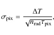
is the integration time per resolution element in the sky.
2.2.1 Angular resolution
The basic scientific requirement for the Planck
angular resolution is to provide
approximately 10' beams in the minimum foreground
window and to achieve up to 5' in the highest frequency
channels. This led to a telescope in the 1.5 m aperture class
to ensure the desired resolution with an adequate rejection of
straylight contamination (Mandolesi et al. 2000a;
Villa
et al. 2002). In general,
a trade-off occurs between main-beam resolution (half-power
beam width, HPBW) and the illumination by the feeds of the edges of
both the primary and sub-reflector (edge taper), which in turn
drives the stray-light contamination effect. An edge taper
>30 dB at an angle of 22![]() and an angular resolution of 14' at 70 GHz were set
as design specifications for LFI. Detailed calculations taking
into account the location of the feeds in the focal plane and the
telescope optical performance (Sandri
et al. 2010) showed that angular resolutions
of
and an angular resolution of 14' at 70 GHz were set
as design specifications for LFI. Detailed calculations taking
into account the location of the feeds in the focal plane and the
telescope optical performance (Sandri
et al. 2010) showed that angular resolutions
of ![]() are achieved for the 70 GHz channels, while at lower
frequencies we expect 24'-28' at 44 GHz
(depending on feed) and
are achieved for the 70 GHz channels, while at lower
frequencies we expect 24'-28' at 44 GHz
(depending on feed) and ![]() at 30 GHz (see also Sect. 7).
at 30 GHz (see also Sect. 7).
2.2.2 Sensitivity
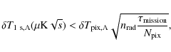
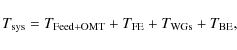
To specify the noise per frequency channel, we adopted the general
criterion of uniform sensitivity per equivalent pixel. In the
early design phases, based on extrapolation of previous technological
progress, we set a noise specification ![]()
![]() 10-6 (or
10-6 (or ![]() K,
thermodynamic temperature) for a reference pixel
K,
thermodynamic temperature) for a reference pixel ![]() at all frequencies. We also considered ``goal'' sensitivities of
at all frequencies. We also considered ``goal'' sensitivities of ![]() K
per reference pixel, i.e., lower by 25%.
K
per reference pixel, i.e., lower by 25%.
With an array of ![]() radiometers at frequency
radiometers at frequency ![]() a sky pixel will be observed, on average, for an
integration time
a sky pixel will be observed, on average, for an
integration time

|
(4) |
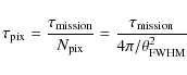
Assuming a 15 month survey, for
As we describe in detail in Sect. 3,
the LFI receivers are coupled in pairs to each feed horn (
![]() )
through an orthomode transducer. Thus the LFI design is such
that all channels are inherently sensitive to polarisation. The
sensitivity to Q and U Stokes
parameters is lower than the sensitivity to total intensity I
by a factor
)
through an orthomode transducer. Thus the LFI design is such
that all channels are inherently sensitive to polarisation. The
sensitivity to Q and U Stokes
parameters is lower than the sensitivity to total intensity I
by a factor ![]() since the number of channels per polarisation is only half
as great. To optimise the LFI sensitivity to
polarisation, the location and orientation of the
LFI radiometers in the focal plan follows well-defined
constraints that are described in Sect. 4.
In Table 1
we summarise the main requirements for LFI sensitivity,
angular resolution, and the nominal LFI design
characteristics.
since the number of channels per polarisation is only half
as great. To optimise the LFI sensitivity to
polarisation, the location and orientation of the
LFI radiometers in the focal plan follows well-defined
constraints that are described in Sect. 4.
In Table 1
we summarise the main requirements for LFI sensitivity,
angular resolution, and the nominal LFI design
characteristics.
Table 1: LFI specifications for sensitivitya and angular resolution.
2.3 Sensitivity budget
For an array of coherent receivers, each with typical
bandwidth ![]() and noise temperature
and noise temperature
![]() ,
observing a sky antenna temperature
,
observing a sky antenna temperature
![]() ,
the average white noise per pixel (in antenna
temperature) will be
,
the average white noise per pixel (in antenna
temperature) will be
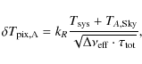
where
where
2.3.1 Bandwidth and system noise
A first breakdown for contributions to LFI sensitivity is
between system temperature and effective bandwidth. Each radiometer is
characterised by a spectral response ![]() that is determined by the overall spectral response of the system
including amplifiers, waveguide components, and filters. We define the
radiometer effective bandwidth as
that is determined by the overall spectral response of the system
including amplifiers, waveguide components, and filters. We define the
radiometer effective bandwidth as
![\begin{displaymath}%
\Delta\nu_{\rm eff}=\frac{\left[\int^\infty_0 g(\nu){\rm d}\nu\right]^2}{\int^\infty_0 g^2(\nu){\rm d}\nu}\cdot
\end{displaymath}](/articles/aa/full_html/2010/12/aa12853-09/img67.png)
In general, therefore, ripples in the band tend to narrow the ideal rectangular equivalent bandwidth. In practice, the effective bandwidth is limited by waveguide components, filters and in-band gain ripples. Extrapolating available technology further, we assume for LFI a goal effective bandwidth of 20% of the central frequency. Equation (5) then leads to requirements on
Table 2: Sensitivity budget for LFI units.
2.3.2 Active cooling
These very ambitious noise temperatures can only be achieved with cryogenically cooled low-noise amplifiers. Typically, the noise temperature of current state-of-the-art cryogenic transistor amplifiers exhibit a factor of 4-5 reduction going from 300 K to 100 K operating temperature, and another factor 2-2.5 from 100 K to 20 K. We implement active cooling to 20 K of the LFI front-end (including feeds, OMTs and first-stage amplification) to gain in sensitivity and to optimise the LFI-HFI thermo-mechanical coupling in the focal plane.
Because the cooling power of the 20 K cooler (see
Sect. 5)
is not compatible with the full radiometers operating at cryogenic
temperature, each radiometer has been split into
a 20 K front-end module and a 300 K
back-end module, each carrying about half of the needed amplification (![]() 70 dB overall).
This solution also avoids the serious technical difficulty of
introducing a detector operating in cryogenic conditions.
A set of waveguides connect the front and back-end modules;
these were designed to provide sufficient thermal decoupling between
the cold and warm sections of the instrument. Furthermore, low power
dissipation components are required in the front-end. This is ensured
by the new generation of cryogenic indium phosphide (InP) high
electron mobility transistor (HEMT) devices, which yield world-record
low-noise performance with very low power dissipation.
70 dB overall).
This solution also avoids the serious technical difficulty of
introducing a detector operating in cryogenic conditions.
A set of waveguides connect the front and back-end modules;
these were designed to provide sufficient thermal decoupling between
the cold and warm sections of the instrument. Furthermore, low power
dissipation components are required in the front-end. This is ensured
by the new generation of cryogenic indium phosphide (InP) high
electron mobility transistor (HEMT) devices, which yield world-record
low-noise performance with very low power dissipation.
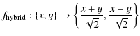
2.3.3 Breakdown allocations
While the system noise temperature, ![]() ,
is dominated by the performance of front-end amplifiers,
additional contributions come from front-end losses and from back-end
noise, which need to be minimised. For each LFI radiometer we can
express the system temperature as
,
is dominated by the performance of front-end amplifiers,
additional contributions come from front-end losses and from back-end
noise, which need to be minimised. For each LFI radiometer we can
express the system temperature as
where the terms on the righthand side represent the contributions from the feed-horn/OMT, front-end module, waveguides, and back-end module. These terms can be expressed as

|
where T0 is the physical temperature of the front end;
In Table 2,
we summarise the main LFI design allocations to the various elements
contributing to the system temperature; these were established by
taking state-of-the-art technology into account.
The contribution from front-end losses,
![]() ,
is reduced to
,
is reduced to
![]() by cooling the feeds and OMTs to 20 K and by using
state-of-the-art low-loss waveguide components. Also,
by requiring 30 dB of gain in the radiometer
front-end, noise temperatures for the back-end module of
by cooling the feeds and OMTs to 20 K and by using
state-of-the-art low-loss waveguide components. Also,
by requiring 30 dB of gain in the radiometer
front-end, noise temperatures for the back-end module of ![]() K
(leading to
K
(leading to ![]() K)
can be acceptable, which allows the use of standard GaAs
HEMT technology for the ambient temperature amplification.
More detailed design specifications for each component are given in
Sect. 4
as we describe the instrument in more detail.
K)
can be acceptable, which allows the use of standard GaAs
HEMT technology for the ambient temperature amplification.
More detailed design specifications for each component are given in
Sect. 4
as we describe the instrument in more detail.
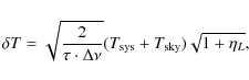
2.4 Stability
Considering perturbations to ideal radiometer stability, the minimum
detectable temperature variation of a coherent receiver is
given by
![\begin{displaymath}%
\delta T(f)=k_R T_{\rm sys}\sqrt{\frac{1}{\tau\cdot \Delta \nu_{\rm eff}}+\left[\frac{\delta G_T(f)}{G_T}\right]^2},
\end{displaymath}](/articles/aa/full_html/2010/12/aa12853-09/img93.png)
where
![\begin{displaymath}%
P(f)\approx \sigma^2 \left[1+\left(\frac{f_{\rm k}}{f}\right)^{\alpha}\right],
\end{displaymath}](/articles/aa/full_html/2010/12/aa12853-09/img97.png)
where
The 1/f noise component not only degrades
the sensitivity but also introduces spurious correlations in the
time-ordered data and sky maps. The reference frequency used to set a
requirement on the knee frequency for LFI is the spacecraft spin
frequency, 1 rpm, or 17 mHz. However,
detailed analyses (Keihänen
et al. 2004; Maino et al. 2002) have
shown that, for the Planck scanning
strategy, a higher knee frequency (
![]() mHz) is acceptable
as robust destriping and map making algorithms can be successfully
applied to suppress the effects of low-frequency fluctuations. Because
a total power HEMT receiver would have typical knee
frequencies of 10 to 100 Hz, a very
efficient differential design is needed for LFI to meet the
50 mHz requirement.
mHz) is acceptable
as robust destriping and map making algorithms can be successfully
applied to suppress the effects of low-frequency fluctuations. Because
a total power HEMT receiver would have typical knee
frequencies of 10 to 100 Hz, a very
efficient differential design is needed for LFI to meet the
50 mHz requirement.
2.5 Systematic effects
Throughout the design and development of LFI a key driver has been the minimisation and control of systematic effects, i.e., deviations from the signal that would be produced by an instrument with axially symmetric Gaussian beams, with ideal pointing and pure Gaussian white noise. These include optical effects (e.g., straylight, misalignment, beam distortions), instrument intrinsic effects (e.g., non-stationary and correlated noise features such as 1/f noise, spikes, glitches, etc.), thermal effects (e.g., temperature fluctuations in the front-end or other instrument interfaces), and pointing errors. In particular, the LFI receiver (discussed in Sect. 3) was designed with the primary objective of minimising the impact of 1/f noise, thermal fluctuations, and systematic effects due to non-ideal receiver components.
The quantitative evaluation of various potential systematic effects required a complex iterative process involving design choices, knowledge and stability of the interfaces (with HFI and with the satellite), testing and modelling of the instrument behaviour, and simulations and simplified data analysis to evaluate the impact of each effect on the scientific output of the mission (Mennella et al. 2004). Furthermore, dedicated analyses were required to evaluate the impact of instrument non-idealities on polarisation measurements (Leahy et al. 2010).
Limits on systematic effects impacting the effective angular
resolution (beam ellipticity, alignment, pointing errors) were used,
together with those coming from HFI, as input to the design of
the Planck telescope and focal plane,
as well as to set pointing requirements at the system level.
Regarding signal perturbations, for LFI we set an upper limit to the
global impact of systematic effects of <3 ![]() K per
pixel at the end of the mission and after data processing. Starting
from this cumulative limit, we defined a breakdown of contributions
from various kinds of effects (Table 3), and then we worked
out more detailed allocations for each contribution. This provided a
useful guideline for the design, development, and testing of the
various LFI subsystems. For each type of systematic error we
specify limits for three cases: a high-frequency component,
spin-synchronous fluctuations, and periodic (non-spin-synchronous)
fluctuations. High-frequency contributions (
K per
pixel at the end of the mission and after data processing. Starting
from this cumulative limit, we defined a breakdown of contributions
from various kinds of effects (Table 3), and then we worked
out more detailed allocations for each contribution. This provided a
useful guideline for the design, development, and testing of the
various LFI subsystems. For each type of systematic error we
specify limits for three cases: a high-frequency component,
spin-synchronous fluctuations, and periodic (non-spin-synchronous)
fluctuations. High-frequency contributions (![]() 0.016 Hz) can be considered as random
fluctuations and added in quadrature to the radiometers' white noise.
As a goal, the overall noise increase due to
random effects other than radiometer white noise should be less
than 10%. Spin synchronous (0.016 Hz) components are
not damped by scanning redundancy, and impose the most stringent limits
on systematic effects. Periodic fluctuations on time scales other than
the satellite spin are damped with an efficiency that depends on the
characteristic time scale of the effect (see Mennella et al. 2002a,
for quantitative analysis). For 1/f and
thermal non-spin-synchronous fluctuations, affecting long time scales,
we set the acceptable limits on systematic effects assuming that a
consolidated destriping algorithm is applied to the data (Maino
et al. 2002,1999).
0.016 Hz) can be considered as random
fluctuations and added in quadrature to the radiometers' white noise.
As a goal, the overall noise increase due to
random effects other than radiometer white noise should be less
than 10%. Spin synchronous (0.016 Hz) components are
not damped by scanning redundancy, and impose the most stringent limits
on systematic effects. Periodic fluctuations on time scales other than
the satellite spin are damped with an efficiency that depends on the
characteristic time scale of the effect (see Mennella et al. 2002a,
for quantitative analysis). For 1/f and
thermal non-spin-synchronous fluctuations, affecting long time scales,
we set the acceptable limits on systematic effects assuming that a
consolidated destriping algorithm is applied to the data (Maino
et al. 2002,1999).
Table 3: Top-level systematic error budget (peak-to-peak values).
High level allocations for signal perturbation effects are indicated in Table 3. The meaning of some of these contributions will become clearer as we provide a description of the design solutions adopted for the LFI instrument and its interfaces (Sects. 4 to 7).
3 Instrument concept
The heart of the LFI instrument is an array of 22 differential receivers based on cryogenic high-electron-mobility transistor (HEMT) amplifiers. Cooling of the front end is achieved by a closed-cycle hydrogen sorption cooler (Morgante et al. 2009), with a cooling power of about 1 W at 20 K, which also provides 18 K pre-cooling to the HFI.
Radiation from the sky intercepted by the Planck telescope is coupled to 11 corrugated feed horns, each connected to a double-radiometer system, the so-called radiometer chain assembly (RCA, see Fig. 1). The complete LFI array, including 11 RCAs and 22 radiometers, is called the radiometer array assembly (RAA).
![\begin{figure}
\par\includegraphics[width=7.5cm,clip]{figures/12853f01.eps}\vspace*{3mm}
\includegraphics[width=8.5cm,clip]{figures/12853f02.ps}
\end{figure}](/articles/aa/full_html/2010/12/aa12853-09/img102.png)
|
Figure 1: Top: schematic of a radiometer chain assembly (RCA). The LFI array has 11 RCAs, each comprising two radiometers carrying the two orthogonal polarisations. The RCA is constituted by a feed horn, an orthomode transducer (OMT), a front-end module (FEM) operated at 20 K, a set of four waveguides that connect FEM to the back-end module (BEM). The notations ``0'' and ``1'' for the two radiometers in the RCA denote the branches downstream of the main and side arms of the OMT, respectively. Each amplifier chain assembly (ACA) comprises a cascaded amplifier and a phase switch. Bottom: picture of a 30 GHz RCA integrated before radiometer-level tests. |
| Open with DEXTER | |
3.1 Radiometer chain assemblies
Downstream of each feedhorn, an orthomode transducer (OMT) separates the signal into two orthogonal polarisations with minimal losses and cross talk. Two parallel, independent radiometers are connected to the output ports of the OMT, thus preserving the polarisation information. Each radiometer pair is split into a front end module (FEM) and a back-end module (BEM) to minimise power dissipation in the actively cooled front end. A set of composite waveguides connect the FEM and the BEM.
The stringent stability requirements are obtained with a pseudo-correlation receiver in which the signal from the sky is continuously compared with the signal from a blackbody reference load. The loads, one for each radiometer, are cooled to approximately 4.5 K by a Stirling cooler that provides the second pre-cooling stage for the HFI bolometers. As we show in detail in Sect. 3.3, each radiometer has two internal symmetric legs, so that each RCA comprises four waveguides connecting the FEM and the BEM and four detector diodes.
Each RCA is designated by a consecutive number (see Sect. 4.1.1). In each RCA, the radiometer connected to the main arm of the OMT is called R0, and the one connected to the side arm is called R1, as shown in Fig. 1. The two detectors in radiometer R0 are named (M-00, M-01), while those in radiometer R1 are named (S-10, S-11).
3.2 Radiometer array assembly
A schematic of the radiometer array assembly (RAA), is shown in Fig. 2. Each RCA has been integrated and tested separately, and then mounted on the RAA without de-integration to ensure stability of the radiometer characteristics after calibration at RCA level (Villa et al. 2010).
A ``mainframe'' supports the LFI 20 K front end (with
feeds, OMTs, and FEMs) and interfaces the HFI 4 K front-end
box in the central portion of the focal plane. The HFI 4 K box
is linked to the 20 K LFI mainframe with insulating
struts and provides the thermal and mechanical interface to the
LFI reference loads. Forty-four waveguides connect the LFI
front-end unit (FEU) to the back-end unit (BEU), which is mounted on
the top panel of the Planck service module (SVM)
and is maintained at a temperature of ![]() K. The BEU comprises
the eleven BEMs and the data acquisition electronics (DAE) unit. After
on-board processing, provided by the radiometer box electronics
assembly (REBA), the compressed signal is down-linked to the ground
station with housekeeping data.
K. The BEU comprises
the eleven BEMs and the data acquisition electronics (DAE) unit. After
on-board processing, provided by the radiometer box electronics
assembly (REBA), the compressed signal is down-linked to the ground
station with housekeeping data.
![\begin{figure}
\par\includegraphics[width=8.5cm,clip]{figures/12853f03}
\end{figure}](/articles/aa/full_html/2010/12/aa12853-09/img104.png)
|
Figure 2: Schematic of the LFI system displaying the main thermal interfaces with the V-grooves and connections with the 20 K and 4 K coolers. Two RCAs only are shown in this scheme. The radiometer array assembly (RAA) is represented by the shaded area and comprises the front-end unit (FEU) and back-end unit (BEU). The entire LFI RAA includes 11 RCAs, with 11 feeds, 22 radiometers, and 44 detectors. |
| Open with DEXTER | |
A major design driver has been to ensure acceptably low conductive and
radiative parasitic thermal loads at the 20 K stage,
particularly those introduced by the waveguides and cryo-harness.
As we discuss below, sophisticated design solutions were
implemented for these units. In addition, three thermal sinks
were used to largely reduce the parasitic loads in the 20 K
stage, and these are the three conical shields (V-grooves) introduced
in the Planck payload module to thermally isolate
the cold telescope enclosure from the SVM at ![]() 300 K
(Tauber
et al. 2010a). The V-grooves also provide multiple
precool temperatures to all of the Planck coolers,
as well as intercepting parasitics from the cooler piping and
HFI equipment. The three V-grooves are expected to reach
in-flight temperatures of approximately 170 K, 100 K,
and 50 K.
300 K
(Tauber
et al. 2010a). The V-grooves also provide multiple
precool temperatures to all of the Planck coolers,
as well as intercepting parasitics from the cooler piping and
HFI equipment. The three V-grooves are expected to reach
in-flight temperatures of approximately 170 K, 100 K,
and 50 K.
The FEU is aligned in the focal plane of the telescope and supported by a set of three thermally insulating bipods attached to the telescope structure. The back-end unit is fixed on top of the Planck service module, below the lower V-groove. In Fig. 3 we show a detailed drawing of the RAA, including an exploded view showing its main subassemblies and units. After integration, the RAA was first tested in a dedicated cryo-facility (Mennella et al. 2010) for instrument level tests (Fig. 4), and then inserted into the payload module after integrating the HFI 4 K box. Figure 5 shows the LFI within the Planck satellite.
![\begin{figure}
\par\includegraphics[width=8.5cm,clip]{figures/12853f04.ps}\vspace*{3mm}
\includegraphics[width=8.5cm,clip]{figures/12853f05.ps}
\end{figure}](/articles/aa/full_html/2010/12/aa12853-09/img105.png)
|
Figure 3: LFI RAA. Top: drawing of the integrated instrument showing the focal plane unit, waveguide bundle and back-end unit. The elements that are not part of LFI hardware (HFI front-end, cooler pipes, thermal shields) are shown in light grey. Bottom: more details are visible in the exploded view, as indicated in the labels. |
| Open with DEXTER | |
![\begin{figure}
\par\includegraphics[width=7.5cm,clip]{figures/12853f06.ps}
\end{figure}](/articles/aa/full_html/2010/12/aa12853-09/img106.png)
|
Figure 4: The LFI instrument in the configuration for instrument level test cryogenic campaign. |
| Open with DEXTER | |
![\begin{figure}
\par\includegraphics[width=7.5cm,clip]{figures/12853f07.ps}
{\hs...
...ludegraphics[width=7cm,clip]{figures/12853f27.ps}\hspace*{0.25cm}}\end{figure}](/articles/aa/full_html/2010/12/aa12853-09/img107.png)
|
Figure 5: Top: schematic of the Planck satellite showing the main interfaces with the LFI RAA on the spacecraft. Bottom: back view of Planck showing the RAA integrated on the PPLM. The LFI Back-end unit is the box below the lowest V-groove and resting on the top panel of the SVM. |
| Open with DEXTER | |
3.3 Receiver design
The LFI receivers are based on an additive correlation concept, or pseudo-correlation, analogous to schemes used in previous applications in early works (Blum 1959), as well as in recent CMB experiments (Jarosik et al. 2003; Staggs et al. 1996). The LFI design introduces new features that optimise stability and immunity to systematics within the constraints imposed by cryogenic operation and by integration into a complex payload such as Planck. The FEM contains the most sensitive part of the receiver, where the pseudo-correlation scheme is implemented, while the BEM provides further RF amplification and detection.
In each radiometer (Fig. 6),
after the OMT, the voltages of the signal from the sky horn, x(t),
and from the reference load, y(t),
are coupled to a 180![]() hybrid that yields
the mixed signals
hybrid that yields
the mixed signals
![]() and
and
![]() at its two output ports. These signals are then amplified by the
cryogenic low-noise amplifiers (LNAs) characterised by noise voltage,
gain, and phase nF1,
gF1,
at its two output ports. These signals are then amplified by the
cryogenic low-noise amplifiers (LNAs) characterised by noise voltage,
gain, and phase nF1,
gF1,
![]() and nF2,
gF2,
and nF2,
gF2,
![]() .
One of the two signals then runs through a switch that shifts the phase
between 0 and 180
.
One of the two signals then runs through a switch that shifts the phase
between 0 and 180![]() at a frequency of 4096 Hz. A second phase
switch is mounted for symmetry and redundancy on the other radiometer
leg, but it does not introduce any switching phase shift. The
signals are then recombined by a second 180
at a frequency of 4096 Hz. A second phase
switch is mounted for symmetry and redundancy on the other radiometer
leg, but it does not introduce any switching phase shift. The
signals are then recombined by a second 180![]() hybrid coupler, thus
producing an output, which is a sequence of signals proportional
to x(t) and y(t)
alternating at twice the phase switch frequency.
hybrid coupler, thus
producing an output, which is a sequence of signals proportional
to x(t) and y(t)
alternating at twice the phase switch frequency.
In the back-end modules (Fig. 6),
the RF signals are further amplified in the two legs of the
radiometers by room temperature amplifiers characterised by noise
voltage, gain and phase nB1,
gB1,
![]() and nB2,
gB2,
and nB2,
gB2,
![]() .
The signals are filtered and then detected by square-law detector
diodes. A DC amplifier then boosts the signal output,
which is connected to the data acquisition electronics. The sky and
reference load DC signals are integrated, digitised, and then
transmitted to the ground as two separated streams of sky and reference
load data.
.
The signals are filtered and then detected by square-law detector
diodes. A DC amplifier then boosts the signal output,
which is connected to the data acquisition electronics. The sky and
reference load DC signals are integrated, digitised, and then
transmitted to the ground as two separated streams of sky and reference
load data.
![\begin{figure}
\par\includegraphics[width=9cm,clip]{figures/12853f08.ps}
\end{figure}](/articles/aa/full_html/2010/12/aa12853-09/img114.png)
|
Figure 6: LFI receiver scheme, shown in the layout of a radiometer chain assembly (RCA). Some details in the receiver components (e.g., attenuators, filters, etc.) differ slightly for the different frequency bands. |
| Open with DEXTER | |
The sky and reference load signals recombined after the second hybrid
in the FEM have highly correlated 1/f fluctuations.
This is because, in each radiometer leg, both the sky
and the reference signals undergo the same instantaneous fluctuations
due to LNAs intrinsic instability. Furthermore, the fast modulation
drastically reduces the impact of 1/f fluctuations
coming from the back-end amplifiers and detector diodes, since the
switch rate ![]() 4 kHz
is much higher than the 1/f knee frequency
of the BEM components. By taking the difference
between the DC output voltages
4 kHz
is much higher than the 1/f knee frequency
of the BEM components. By taking the difference
between the DC output voltages
![]() and
and
![]() ,
therefore, the 1/f noise is
highly reduced.
,
therefore, the 1/f noise is
highly reduced.
Differently from the WMAP receivers, the LFI phase switches and second hybrids have been placed in the front end. This allows full modularity of the FEMs, BEMs, and waveguides, which in turns simplifies the integration and test procedure. Furthermore, this design does not require that the phase be preserved in the waveguides, a major advantage given the complex routing imposed by the LFI-HFI integration and the potentially significant thermo-elastic effects from the cryogenic interfaces in the Planck payload.
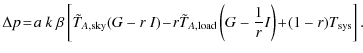
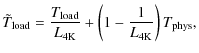
In principle, for a null differential output corresponding to
a perfectly balanced system, fluctuations would be fully suppressed in
the differenced data. In practice, for LFI,
a residual offset will be necessarily present due to input
asymmetry between the sky arm (![]() K from the sky,
plus
K from the sky,
plus ![]() 0.4 K
from the reflectors) and the reference load arm (with physical
temperature
0.4 K
from the reflectors) and the reference load arm (with physical
temperature ![]() 4.5 K),
plus a small contribution from inherent radiometer asymmetry.
To compensate for this effect, a gain modulation
factor r is introduced in software to null
the output by taking the difference
4.5 K),
plus a small contribution from inherent radiometer asymmetry.
To compensate for this effect, a gain modulation
factor r is introduced in software to null
the output by taking the difference ![]() .
In the next section, we discuss the signal model in
more detail.
.
In the next section, we discuss the signal model in
more detail.
![\begin{figure}
\par\includegraphics[width=15cm,clip]{figures/12853f28.eps}
\end{figure}](/articles/aa/full_html/2010/12/aa12853-09/img119.png)
|
Figure 7:
Curves of equal |
| Open with DEXTER | |
3.3.1 Signal model
If x(t) and y(t) are the input voltages at each component, then the transfer functions for the hybrids, the front-end amplifiers, the phase switches, and the back-end amplifiers can be written, respectively, as
where
For small phase mismatches and assuming negligible phase
switch imbalance, the power output of the differenced signal after
applying the gain modulation factor is given by
In Eq. (12) a is the proportionality constant of the square-law detector diode, and G and I are the effective power gain and isolation of the system:
where gB is the voltage gain of the BEM in the considered channel. In Eq. (12) the temperature terms,
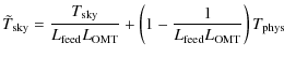
represent the sky and reference load signals at the input of the first hybrid, where
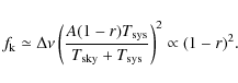
3.3.2 Knee frequency and gain modulation factor
For a radiometer with good isolation (>13 dB),
as expected in a well-matched system, it follows from
Eq. (12)
that the power output is nullified for
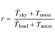
In this case the gain fluctuations are fully suppressed and the radiometer is only sensitive to the 1/f noise caused by noise temperature fluctuations, which only represents a small fraction of the amplifiers instability. For an optimal choice of the gain modulation factor, the resulting knee frequency is given by
Thus, in principle, for small input offsets
It is essential that the gain modulation factor r
be calculated with sufficient precision to reach the required
stability. Simulations and testing show that the needed accuracy ranges
from ![]() (30 GHz) to
(30 GHz) to
![]() (70 GHz). This accuracy can be obtained with different methods
(Mennella et al. 2003),
the simplest being to evaluate the ratio of the total power output
voltages averaged over a suitable time interval,
(70 GHz). This accuracy can be obtained with different methods
(Mennella et al. 2003),
the simplest being to evaluate the ratio of the total power output
voltages averaged over a suitable time interval, ![]() .
In Fig. 8
we show, as an example, the data streams from one of
the 44 LFI detectors with the two total power signals
and differenced data. The LFI telemetry allocations ensure that the
total power data from both the sky and reference load samples will be
downloaded, so calculation of r and
differencing is performed on the ground.
.
In Fig. 8
we show, as an example, the data streams from one of
the 44 LFI detectors with the two total power signals
and differenced data. The LFI telemetry allocations ensure that the
total power data from both the sky and reference load samples will be
downloaded, so calculation of r and
differencing is performed on the ground.
Further suppression of common fluctuation modes, typically of thermal or electrical origin, is obtained by taking the noise-weighted average of the two detectors associated to each radiometer (Mennella et al. 2010) as well as in the differencing of the main and side arm radiometers signals when analysing data for polarisation (Leahy et al. 2010).
![\begin{figure}
\par\includegraphics[width=7.5cm,clip]{figures/12853f09.ps}
\end{figure}](/articles/aa/full_html/2010/12/aa12853-09/img143.png)
|
Figure 8: Example of uncalibrated data stream from one of the 44 LFI detectors (LFI19M-00, at 70 GHz) recorded during instrument level tests. The upper and middle panels show the data for the sky and reference load inputs, while the lower panel shows differenced data stream with optimal gain modulation factor. |
| Open with DEXTER | |
![\begin{figure}
\par\includegraphics[width=18cm,clip]{figures/12853f29.ps}
\end{figure}](/articles/aa/full_html/2010/12/aa12853-09/img144.png)
|
Figure 9: Schematics of the LFI showing interconnections and details of the DAE and REBA main functions and units. |
| Open with DEXTER | |
3.3.3 Noise temperature
The LFI radiometer sensitivity is essentially independent of the
temperature of the reference loads. From Eqs. (5)
and (12)
it follows that, to first order, the radiometer
sensitivity is
where

and TN,B is the noise temperature of the back-end, and GF the gain of the front end. For parameter values typical of LFI, we have
4 LFI configuration and subsystems
The overall LFI system is shown schematically in Fig. 9. In this section we provide an overview of the instrument units and main subsystems. More details on the design, development and testing of the most critical components are given in companion papers that are cited below.
4.1 The front-end unit
4.1.1 Focal plane design
The disposition of the LFI feeds in the focal plane is driven by optimisation of angular resolution and by recovery of polarisation information. In addition, requirements need to be met on proper sampling of the sky and rejection of crosstalk effects.
The central portion of the Planck focal plane is occupied by the HFI front end, as higher frequency channels are more susceptible to optical aberration. The LFI feeds are located as close as possible to the focal plane centre compatible with mechanical interfaces with HFI and 4 K reference loads (Fig. 10). Miniaturised designs for the FEMs and OMT are implemented to allow optimal use of the focal area. The 70 GHz feeds, most critical for cosmological science, are placed in the best location for angular resolution and low beam distortion required for this frequency (Sandri et al. 2010).
A key criterion for the feed arrangement is that the E
and H planes as projected in the sky will
allow optimal discrimination of the Stokes Q
and U parameters. The polarisation
information is obtained by differencing the signal measured by the
main-arm (R0) and side-arm (R1) radiometers in each RCA, which are set
to 90![]() angle
by the OMT. An optimal extraction of Q
and U is achieved if subsets of channels
are oriented in such a way that the linear polarisation directions are
evenly sampled (Leahy
et al. 2010). We achieve this by arranging pairs of
feeds with their E planes oriented
at 45
angle
by the OMT. An optimal extraction of Q
and U is achieved if subsets of channels
are oriented in such a way that the linear polarisation directions are
evenly sampled (Leahy
et al. 2010). We achieve this by arranging pairs of
feeds with their E planes oriented
at 45![]() to each other (Fig. 11).
With the exception of one 44 GHz feed, all the E planes
are oriented at
to each other (Fig. 11).
With the exception of one 44 GHz feed, all the E planes
are oriented at ![]() 22.5
22.5![]() relative to the scan direction. We also align pairs of feeds such that
their projected lines of sight will follow each other in the Planck
scanning strategy.
relative to the scan direction. We also align pairs of feeds such that
their projected lines of sight will follow each other in the Planck
scanning strategy.
![\begin{figure}
\par\includegraphics[width=7.5cm,clip]{figures/12853f10.ps}\vspace*{3mm}
\includegraphics[width=7.5cm,clip]{figures/12853f11.ps}
\end{figure}](/articles/aa/full_html/2010/12/aa12853-09/img149.png)
|
Figure 10: Arrangement of the LFI feeds in the focal plane. Top: mechanical drawing of the main frame and focal plane elements. Shown are the bipods connecting the FPU to the telescope structure. Bottom: picture of the LFI flight model focal plane. |
| Open with DEXTER | |
![\begin{figure}
\par\includegraphics[width=7.5cm,clip]{figures/12853f12.eps}
\end{figure}](/articles/aa/full_html/2010/12/aa12853-09/img152.png)
|
Figure 11:
Footprint of the LFI main beams on the sky and polarisation angles as
seen by an observer looking towards the satellite along its optical
axis. The units are u-v coordinates
defined as |
| Open with DEXTER | |
The spin axis of Planck will be shifted by 2' every
![]() 45 min
(Tauber
et al. 2010a). Therefore, even for the highest
LFI angular resolution,
45 min
(Tauber
et al. 2010a). Therefore, even for the highest
LFI angular resolution, ![]() at 70 GHz, the sky is well sampled.
at 70 GHz, the sky is well sampled.
4.1.2 LFI main frame
The LFI mainframe provides thermo-mechanical support to the LFI radiometer front-end, but it also supports the HFI and interfaces to the cold end (nominal and redundant) of the 20 K sorption cooler. In fact, some of the key requirements on the LFI mainframe (stiffness, thermal isolation, optical alignment) are driven by the HFI rather than the LFI instrument. The mainframe is built of the aluminium alloy 6061-T6, and it is dismountable in three subunits to facilitate integration of the complete RCAs and of the HFI front-end.
The interface between the FPU and the 50 K payload
module structure must ensure thermal isolation, as well as compliance
with eigenfrequencies from launch loads. A trade-off was made
to identify the proper material properties, fibre orientations, and
strut inclinations. The chosen configuration was a set of three
225-mm-long CFRP T300 bipods, inclined at 50![]() .
The LFI-HFI interface is provided by a structural ring connected to the
HFI by six insulating struts locked to the LFI main frame through a
shaped flange. The design of the interface ring allows
HFI integration inside the LFI, as well as
waveguide paths, while ensuring accurate alignment of the 4 K
reference loads with the reference horns mounted on the FEMs.
.
The LFI-HFI interface is provided by a structural ring connected to the
HFI by six insulating struts locked to the LFI main frame through a
shaped flange. The design of the interface ring allows
HFI integration inside the LFI, as well as
waveguide paths, while ensuring accurate alignment of the 4 K
reference loads with the reference horns mounted on the FEMs.
4.1.3 Feed horns
The LFI feeds must have highly symmetric beams, low levels of side
lobes (-35 dB), cross-polarisation (-30 dB), and
return loss (-25 dB), as well as good control of the
phase centre location (Villa
et al. 2002). Dual profiled conical corrugated horns
have been designed to meet these requirements, a solution that
has the added advantage of high compactness and design flexibility. The
profiles have a sine squared inner section, i.e.,
![]() ,
and by an exponential outer section,
,
and by an exponential outer section, ![]() .
.
The detailed electromagnetic designs of the feeds were developed based on the entire optical configuration of the feed-telescope system. The control of the edge taper only required minimal changes on the feed aperture and overall feed sizes, so that an iterative design process could be carried out at system level.
The evaluation of straylight effects in the optimisation process required extensive simulations (carried out with GRASP8 software) of the feed-telescope assembly for several different feed designs, edge tapers, and representative positions in the focal plane (Sandri et al. 2010). A multi-GTD (geometrical theory of diffraction) approach was necessary since the effect of shields and multiple scatter needed to be included in the simulations. In Table 4 we report the main requirements and characteristics of the LFI feed horns. The details of the design, manufacturing, and testing of the LFI feed horns are discussed in Villa et al. (2009b).
Table 4: Specifications of the feed horns.
4.1.4 Orthomode transducers
The use of orthomode transducers (OMTs) allows the full power intercepted by the feed horns to be used by the LFI radiometers, and makes each receiver intrinsically sensitive to linear polarisation. The OMT splits the TE11 propagation mode from the output circular waveguide of the feed horn into two orthogonal polarised components. Low insertion loss (<0.15 dB) is needed to minimise any impact on radiometer sensitivity. In addition, OMTs are critical components for achieving the ambitious wide bandwidth specification, especially when combined with the miniaturisation imposed by the focal plane arrangement.
Table 5: Specifications of the OMTs.
These requirements made commercial OMTs inadequate for LFI, and a dedicated design development was carried out for these components (Villa et al. 2009a). An asymmetric design was selected, with a common polarisation section connected to the feed horn and to the main and side arms in which the two polarisations are separated. A modular design approach was developed, in which six different sections were identified, each corresponding to a specific electromagnetic function. While the basic configuration of the OMTs at different frequencies is scaled from a common design, some details are optimised depending on frequency, such as the location of the waveguide twist in the side arm or in the main arm. The main design specifications for the LFI orthomode transducers are given in Table 5. Detailed discussion of the design, manufacturing, and unit-level testing of the LFI OMTs are reported in Villa et al. (2009a).
4.1.5 Front-end modules
The performance of the LFI relies largely on its front-end modules (FEMs, see Table 6). Detailed descriptions of the 30 GHz and 44 GHz FEMs are given by Davis et al. (2009), and of the 70 GHz FEMs by Varis et al. (2009). Each FEM accepts four input signals, two from the rectangular waveguide outputs of the OMT and two from the 4 K reference loads viewed by rectangular horns attached to the FEMs (Fig. 6).
In each half-FEM, the sky and reference input signals were connected to a hybrid coupler (or ``magic-T''). To minimise front-end losses, waveguide couplers were used, machined in the aluminium-alloy FEM body and gold-plated. At 20 K the hybrid losses were estimated 0.1 to 0.2 dB. The first hybrid divides the signals between two waveguide outputs along which the low noise amplifiers (LNAs) and phase shifters were mounted. The internal waveguide design ensured that the phase is preserved at the input of the second hybrid. The signals were thus recombined at the FEM outputs as voltages that are proportional to the sky or reference load signal amplitude, depending on the state of the modulated phase switches.
At 70 GHz the large number of channels called for a highly modular FEM design, where each half-module can be easily dismounted and replaced. In addition, the elements hosting the LNAs and the phase shifters (the so-called amplifier chain assembly, ACA, see Fig. 1) are built as separable units. This allowed flexibility during selection and testing, which proved extremely useful when replacement with a spare unit was required in an advanced stage of integration (Mennella et al. 2010). At 30 and 44 GHz, a multi-splitblock solution was devised to facilitate testing and integration, in which the four ACAs were mounted to end plates and arranged in a mirror-image format.
Table 6: Specifications of the front-end modules.
LNAs.
To meet LFI requirements it was necessary to reach lower amplifier noise temperatures than previously achieved with multi-stage transistor amplifiers. We implemented state-of-the art cryogenic InP HEMT technology at all frequencies. Each front-end LNA must have a minimum of 30 dB of gain to reject back-end noise, which required 4 to 5 stage amplifiers. In addition to low noise, the InP technology enables very low-power operation, which is essential for meeting the requirements for heat load at 20 K. The amplifiers were selected and tuned for best operation at low drain voltages and for gain and phase match between paired radiometer legs, which is crucial for good balance.The 70 GHz receivers were based on monolithic
microwave integrated circuit (MMIC) semiconductors (Fig. 14) while discrete
HEMTs on a substrate (MIC technology) were used at 30
and 44 GHz. To reach lowest possible noise
temperatures, ultra-short gate devices are adopted. The final design
used 0.1 ![]() m
gate length InP HEMTs manufactured by TRW (now Northrop Grumman) from
the Cryogenic HEMT Optimisation Programme (CHOP).
m
gate length InP HEMTs manufactured by TRW (now Northrop Grumman) from
the Cryogenic HEMT Optimisation Programme (CHOP).
Phase shifters.
After amplification, the LNA output signals are applied to two identical phase shifters whose state is set by a digital control line modulated at 4 kHz. The signal is then conveyed via stripline to waveguide transitions to the second hybrid, and then passes to the interface with the interconnecting waveguide assembly to the BEMs. The phase switch design used at all frequencies is based on a double hybrid-ring configuration (Hoyland 2003). The switches, manufactured with InP PIN diodes, have demonstrated excellent cryogenic performances for low 1/f noise contribution and good 180Electrical connections.
Each of the 11 FEMs uses 16 to 20 low noise transistors and 8 phase-switch diodes, all operated in cryo conditions. This sets demanding requirements in the design of the bias circuitry. The LNA biases are controlled by the data acquisition electronics (DAE) to obtain the required amplification and lowest noise operation. Different details in the design of the FEMs at each frequency minimise the number of supply lines. In the 30 and 44 GHz FEMs, potentiometers were used to simplify the control wiring. The cryo-harness wiring that connects the FEMs to the power supply isProper tuning of the LNAs is critical for best performance.
The front-end InP LNAs contain 4 stages of amplification
at 30 and 70 GHz and 5 stages
at 44 GHz. The LNAs are driven by three voltages:
a common drain voltage (![]() ), a gate voltage for
the first stage (
), a gate voltage for
the first stage (
![]() ), and a common gate voltage
for the remaining stages (
), and a common gate voltage
for the remaining stages (
![]() )
(Fig. 15).
The voltages
)
(Fig. 15).
The voltages
![]() and
and ![]() are programmable and are optimised in the tuning phase (Cuttaia et al. 2009).
The total drain current,
are programmable and are optimised in the tuning phase (Cuttaia et al. 2009).
The total drain current, ![]() flowing in the ACA
is measured and is available in the instrument housekeeping.
flowing in the ACA
is measured and is available in the instrument housekeeping.
4.2 The 4 K reference load system
Blackbody loads provide stable internal signals for the
pseudo-correlation receivers (Valenziano
et al. 2009). Cooling the loads as close as possible
to the ![]() 3 K
sky temperature minimises the radiometer knee frequency (Eq. (16)) and
reduces the susceptibility to thermal fluctuations and to other
systematic effects. Requirements are thus derived for the loads'
absolute temperature,
3 K
sky temperature minimises the radiometer knee frequency (Eq. (16)) and
reduces the susceptibility to thermal fluctuations and to other
systematic effects. Requirements are thus derived for the loads'
absolute temperature, ![]() K,
as well as for the insertion loss of the reference horn,
K,
as well as for the insertion loss of the reference horn, ![]() dB.
dB.
Connecting the loads to the HFI 4 K stage imposes
challenging thermo-mechanical requirements on the system. The loads
must be thermally isolated from, but radiometrically
matched to, the reference horns feeding the
20 K FEMs. Complete thermal decoupling is obtained by
leaving a ![]() 1.5 mm
gap between the loads and the reference horns.
1.5 mm
gap between the loads and the reference horns.
![\begin{figure}
\par\includegraphics[width=7.5cm,clip]{figures/12853f13.ps}
\end{figure}](/articles/aa/full_html/2010/12/aa12853-09/img162.png)
|
Figure 12: Picture of nine of the eleven feed horns and associated OMTs, FEMs, and waveguides before integration of the HFI front end. The six smaller feeds in the front supply the 70 GHz channels. In the back row, the two 30 GHz feeds flank one of the 44 GHz feeds. Visible are part of the twisted Cu waveguide sections and the reference horns (protected by a kapton layer): for the 70 GHz FEMs they are embodied in the FEMs, while for the 30 and 44 GHz they are flared waveguide sections. |
| Open with DEXTER | |
![\begin{figure}
\par\includegraphics[width=7.5cm,clip]{figures/12853f14.ps}\par\includegraphics[width=7.5cm,clip]{figures/12853f15.ps}
\end{figure}](/articles/aa/full_html/2010/12/aa12853-09/img163.png)
|
Figure 13: Top: structure of a 70 GHz half-FEM. On the right side of the module, one can see the small reference horn used to couple to the 4 K reference load surrounded by quarter-wave grooves. The parts supporting the amplifier chain assembly are dismounted and shown in the front. Bottom: picture of LNA and phase switch within a 30 GHz FEM. The RF channel incorporating the four transistors runs horizontally in this view. The phase switch is the black rectangular element on the left. |
| Open with DEXTER | |
| Figure 14:
A 4-stage InP HEMT MMIC low-noise amplifier used in a flight model FEM
at 70 GHz. The size of the MMIC is 2.1 mm |
|
| Open with DEXTER | |
![\begin{figure}
\par\includegraphics[width=7.5cm,clip]{figures/12853f17.ps}
\end{figure}](/articles/aa/full_html/2010/12/aa12853-09/img165.png)
|
Figure 15: DAE biasing to a front-end LNA. Each LNA is composed of four to five amplifier stages driven by a common drain voltage, a dedicated gate voltage to the first stage (most critical for noise performances), and a common gate voltage to the other stages. |
| Open with DEXTER | |
![\begin{figure}
\par\includegraphics[width=7.5cm,clip]{figures/12853f18.ps}
\end{figure}](/articles/aa/full_html/2010/12/aa12853-09/img166.png)
|
Figure 16: Picture of the reference loads mounted on the HFI 4 K box. On the top is the series of loads serving the 70 GHz radiometers, while in the lower portion are the loads of the two 30 GHz FEMs and one of the 44 GHz FEMs. Each FEM is associated to two loads, each feeding a radiometer in the RCA. |
| Open with DEXTER | |
Radiometric requirements for the loads were derived by analysis and tests (Valenziano et al. 2009). The coupling between the reference horns and the loads is optimized to reduce reflectivity and to avoid straylight radiation leaking through the gap, with a required match at the horn aperture >20 dB. For the 70 GHz radiometers the reference horns are machined as part of the FEM body, while for the 30 and 44 GHz they are fabricated as independent waveguide components and mounted on the FEM (Fig. 12). This is because of the different paths required to reach the loads, whose location on the 4 K box is constrained by the LFI-HFI interface.
The configuration of the loads is the result of a complex trade-off between RF performance and a number of constraints such as allowed mass, acceptable thermal load on the 4 K stage, and available volume. The latter is limited by the optical requirement of placing the sky horns close to the focal plane centre. In addition, the precise location and alignment of the loads on the HFI box need to follow the non-trivial orientation and arrangement of the FEMs, dictated by the optical requirements for angular resolution and polarisation. The final design comprises a front layer (made in ECR-110) shaped for optimal match with the reference horn radiation pattern and a back layer (ECR-117) providing excellent absorption efficiency.
Requirements on thermal stability at the 4 K shield
interface were set to ![]() K
K![]() ,
i.e., at the same level as the HFI internal requirement. To
maximise thermal stability, a PID (proportional, integral, and
derivative) system was implemented on the HFI 4 K box (Lamarre et al. 2010).
The 70 GHz loads are located near the top of the HFI
4 K box, near the PID control system, while the 30
and 44 GHz loads are in the lower part (Figs. 12 and 16).
This resulted in a more stable signal for the LFI 70 GHz loads
than for the 30 and 44 GHz ones. Simulations have
shown that residual systematic effects on the maps at end-of-mission,
after applying destriping algorithms (Keihänen
et al. 2004), are expected to be
,
i.e., at the same level as the HFI internal requirement. To
maximise thermal stability, a PID (proportional, integral, and
derivative) system was implemented on the HFI 4 K box (Lamarre et al. 2010).
The 70 GHz loads are located near the top of the HFI
4 K box, near the PID control system, while the 30
and 44 GHz loads are in the lower part (Figs. 12 and 16).
This resulted in a more stable signal for the LFI 70 GHz loads
than for the 30 and 44 GHz ones. Simulations have
shown that residual systematic effects on the maps at end-of-mission,
after applying destriping algorithms (Keihänen
et al. 2004), are expected to be ![]() K at
30-44 GHz and
K at
30-44 GHz and ![]() K
at 70 GHz.
K
at 70 GHz.
4.3 Waveguides
A total of 44 waveguides connect the 20 K FEU and the 300 K BEU through a length of 1.5 to 1.9 m, depending on RCA. Conflicting constraints of thermal, electromagnetic, and mechanical nature imposed challenging trade-offs in the design. The LFI waveguides must ensure good thermal isolation between the FEM and the BEM, while avoiding excessive attenuation of the signal. In addition, their mechanical structure must comply with the launch vibration loads. The asymmetric location of the FEMs in the focal plane and the need to ensure integrability of the HFI in the LFI main frame, as well as of the RAA on the spacecraft, impose complex routing with several twists and bends, which required a dedicated design for each individual waveguide.
| Figure 17: Schematics of the LFI composite waveguide design, showing representative dimensions of the various sections as described in the text. |
|
| Open with DEXTER | |
![\begin{figure}
\par\includegraphics[width=7.5cm,clip]{figures/12853f20.ps}\vspace*{3mm}
\includegraphics[width=7.5cm,clip]{figures/12853f21.ps}
\end{figure}](/articles/aa/full_html/2010/12/aa12853-09/img172.png)
|
Figure 18: Pictures of the LFI waveguides mounted on the RAA during the integration of the LFI flight model. Top: a view of the straight SS sections, black-painted on the outside and arranged in groups of four. On the upper part the Cu sections are connected through multiple flanges. The upper and lower mechanical support structures are also visible. The three interface levels corresponding to the three V-grooves are also shown. Bottom: back view of the LFI front-end unit showing the twisted Cu sections connecting to the FEMs. The waveguide routing and central hole in the main frame are designed to interface with the HFI front-end 4 K box. |
| Open with DEXTER | |
Table 7: RF requirements on the waveguides.
A composite configuration was devised with two separated sections: a stainless steel (SS) straight section connecting to the BEMs, and a copper (Cu) section incorporating all the twists and bends and connecting to the FEMs (Fig. 17). The two sections are connected via custom-designed multiple flanges, each serving the four guides in each RCA.
The SS sections essentially support the entire
20-300 K thermal gradient. All
44 SS waveguides have the same length
(70 cm) and are gold-plated (2 ![]() m thickness) in the first 40 cm near the
BEM interface to minimise ohmic losses. They are thermally
sunk to the three V-grooves (Fig. 18),
and their outer surfaces are painted black
(Aeroglaze Z306) to optimise heat radiation.
m thickness) in the first 40 cm near the
BEM interface to minimise ohmic losses. They are thermally
sunk to the three V-grooves (Fig. 18),
and their outer surfaces are painted black
(Aeroglaze Z306) to optimise heat radiation.
The Cu sections, of lengths 80 to 120 cm depending on RCA, operate at a nearly constant temperature of 20 K, and are individually designed based on optimisation of return loss compatible with the required routing. Precise criteria for the curvature radii, twist length, and mechanical tolerances were followed in the design (D'Arcangelo et al. 2009). Dynamical analysis showed the need for two dedicated mechanical support structures to ensure compliance with the vibration loads of the Ariane 5 launch (Fig. 18).
The selected design proved to meet simultaneously the heat load limits to the 20 K stage (250 mW for the bundle of 44 guides) and the insertion loss at a level of few dBs. A thermal model was developed to calculate the temperature profile along the waveguide and the final solution was found using an analytical model.
D'Arcangelo et al. (2009) gives a full account of the manufacturing, qualification, and challenging test plan of the LFI waveguides.
4.4 Back-end unit
4.4.1 Back-end modules
The back-end modules (BEMs) are housed in the LFI back-end unit,
together with the DAE, and are operated at room temperature ![]() 300 K.
Each BEM has four branches, grouped in pairs (Fig. 6).
In each channel within the BEM, the incoming signal is
filtered by a band-pass filter, amplified by cascaded transistor
amplifiers, detected by a detector diode, and DC-amplified. The BEM
casing also incorporates bias and protection circuits and connectors.
Room temperature noise figures <3 dB and an overall
amplification of 20 to 25 dB, depending on RCA, are
specified for the BEM channels. Amplifier and detector diode
instabilities are efficiently removed by the 4 kHz phase
switching, so that amplifier knee frequencies of
300 K.
Each BEM has four branches, grouped in pairs (Fig. 6).
In each channel within the BEM, the incoming signal is
filtered by a band-pass filter, amplified by cascaded transistor
amplifiers, detected by a detector diode, and DC-amplified. The BEM
casing also incorporates bias and protection circuits and connectors.
Room temperature noise figures <3 dB and an overall
amplification of 20 to 25 dB, depending on RCA, are
specified for the BEM channels. Amplifier and detector diode
instabilities are efficiently removed by the 4 kHz phase
switching, so that amplifier knee frequencies of ![]() 100 Hz
are acceptable.
100 Hz
are acceptable.
Amplifiers.
The 30 and 44 GHz BEMs (Artal et al. 2009) use MMIC gallium arsenide (GaAs) amplifiers. Each LNA consists of two cascaded stages. The 30 GHz MMICs are commercial circuits using four stages of pseudomorphic HEMTs with an operating bandwidth from 24 to 36 GHz, 23 dB of gain, and a 3 dB noise figure. The 44 GHz MMICs were manufactured with a process employing a 0.2Band pass filters.
Band pass filters in the BEMs were used to define the bandwidth and to reject out-of-band parasitic signals. In the 30 and 44 GHz units the filter is based on a microstrip-coupled line structure that inherently provides bandpass characteristics. Waveguide filters are used at 70 GHz, where the wavelength-scale cavity has an acceptable size.Detector diodes
The detector design at 30 and 44 GHz uses commercially available GaAs planar doped-barrier Schottky diodes. The diodes were mounted with a coplanar-to-microstrip transition to facilitate on-wafer testing prior to integration in the BEM. As in the FEM design, at 70 GHz the filters and the amplifier-detector assemblies of paired channels were mounted on separable modules to offer greater flexibility in the testing and optimisation phases.DC amplifiers
The detector diode is followed by a low-noise DC-amp with a voltage gain adequate to the required analogue output voltage range for the DAE interface. To meet EMC requirements and grounding integrity, the output voltages are provided as differential signals.![\begin{figure}
\par\includegraphics[width=7.5cm,clip]{figures/12853f22.ps}
\end{figure}](/articles/aa/full_html/2010/12/aa12853-09/img173.png)
|
Figure 19: Picture of the lower part of the LFI RAA during an advanced phase of the instrument flight-model integration showing the LFI back-end unit. The two lateral trays hosting the radiometer BEMs are symmetrically disposed to the left and right sides of the DAE-BEU box. The lower part of the straight stainless steel waveguides are shown. |
| Open with DEXTER | |
4.4.2 Data acquisition electronics
The acquisition and conditioning of the science signals from the BEMs and of housekeeping data is performed by the data acquisition electronics. The DAE also provides power supply, conditioning, and distribution to the RAA, in particular DC biasing to the LNAs and phase switches in the FEMs, as well as to the BEM amplifiers. The DAE tags the acquired data using the information of its on-board time to ensure that correlation can be made on the ground for proper pointing reconstruction. The raw data are then transmitted to the science processing unit for on-board processing.
As shown schematically in Fig. 9, the DAE functions are distributed into different sub-units. The ``DAE-BEU box'' and the ``lateral trays'' incorporate all the main functions, and are located in the back-end unit with the radiometer BEMs (Fig. 19). A separate ``DAE power box'' is interfaced with the spacecraft in order to receive the primary power supply and generate the needed secondary voltages to the DAE.
The DAE-BEU box is in charge of conditioning and acquiring the science data. The signals coming from the 44 detectors are integrated and held during the synchronous sampling and conversion. Science signals are digitised with 14-bit analogue-to-digital converters using a successive approximation conversion algorithm. There are 44 independent analogue acquisition chains, one for each detector arm. To optimise the analogue signals from the BEMs to the ADC dynamic range, dedicated circuits remove an offset and then amplify the DC signal. Both offset and gain are programmable and are optimised as part of the instrument calibration process (Cuttaia et al. 2009; Mennella et al. 2010). In the optimised configuration, the number of counts exercised by the radiometer noise varies from 10 to 450, depending on channel. Acquired data are converted into serial streams and automatically transferred to the signal-processing unit in the REBA through synchronous serial links for processing and compression (Sect. 4.5).
The DAE is also in charge of collecting and storing housekeeping data in a dedicated RAM. This information is retrieved by the REBA and organised into two dedicated packets with periods of 1 and 32 s, depending on the needed monitoring frequency. Housekeeping parameters include current consumptions in the FEMs and temperature sensors, which are essential for trend analysis and systematic error tests. These data are used extensively during the functionality checks of the radiometers.
The two DAE ``lateral trays'' contain the circuitry needed to provide the power supply to the RCAs, divided into four power groups (Fig. 9). These power supplies are independent of each other to minimise crosstalk and interference. The bias of each FEM and the controls for the phase switches are regulated to selectable voltage levels and filtered to achieve a minimum level of conducted noise. Particularly critical for the instrument performance is the optimal biasing of the FEM amplifiers. As described in Sect. 4.1.5, the bias voltages of the first LNA stage and of the following stages are programmable separately.
4.5 Radiometer electronics box (REBA)
Downstream of the DAE, the LFI signals are digitally processed by the REBA (radiometer electronics box assembly), which also contains the power supply for LFI and the interface with the satellite SVM. The electronics hardware and on-board software are discussed by (Herreros et al. 2009). The REBA is a fully redundant unit, and it is internally separated into different subunits as shown schematically in Fig. 9.
The signal processing unit (SPU) receives the raw digital
science data from the DAE and performs on-board signal averaging, data
compression, and science telemetry packetisation. The need to reject 1/f noise
led to raw data sampling at 8192 Hz (122![]() s/sample),
the LFI internal clock generator frequency. The clock
synchronously drives the phase switches in the FEMs, the ADCs, and the
on-board processor, which reconstructs the ordering of the acquired
signals and synchronises it with the on-board time. Taking housekeeping
and ancillary information into account, this corresponds to a data rate
of
s/sample),
the LFI internal clock generator frequency. The clock
synchronously drives the phase switches in the FEMs, the ADCs, and the
on-board processor, which reconstructs the ordering of the acquired
signals and synchronises it with the on-board time. Taking housekeeping
and ancillary information into account, this corresponds to a data rate
of ![]() 5.7 Mbps,
or a factor of 100 higher than the allocated
data rate for the instrument, 53.5 Kbps. Averaging the samples
from sky and reference-load signals to within the Nyquist rate on the
sky (3 bins per HPBW at each frequency) drastically reduces
the data volume, leaving a compression requirement of a
factor 2.4 (see Sect. 6).
The adopted algorithm implemented in the SPU relies on three-step
processing of nearly loss-less compression that requires 5-parameter
tuning to be optimised. The details of the LFI data
compression strategy and end-to-end test results are discussed by Maris et al. (2009).
5.7 Mbps,
or a factor of 100 higher than the allocated
data rate for the instrument, 53.5 Kbps. Averaging the samples
from sky and reference-load signals to within the Nyquist rate on the
sky (3 bins per HPBW at each frequency) drastically reduces
the data volume, leaving a compression requirement of a
factor 2.4 (see Sect. 6).
The adopted algorithm implemented in the SPU relies on three-step
processing of nearly loss-less compression that requires 5-parameter
tuning to be optimised. The details of the LFI data
compression strategy and end-to-end test results are discussed by Maris et al. (2009).
The main functions of the data processing unit (DPU) include monitoring and control of the RAA, instrument initialisation, error management, on-board time synchronisation, management of instrument operating modes, and control of the overall LFI data rate and data volume. Switching the FEMs and BEMs on and off, as well as voltage adjustments, are addressed by the DPU with a configuration that allows flexible setup commands. The DPU interface provides all commands for the DAE, while the SPU interface is in charge of retrieving the fixed format raw data from the RCAs. Both the DPU and the SPU are based on an 18 MHz CPU. The link between the REBA and the DAE is implemented through IEEE 1355 interfaces and by means of data flag signals that ensure hardware and software synchronisation.
Finally, the data acquisition unit (DAU) is in charge of functions that are internal to the REBA, and it has no interfaces with the RAA. It converts the primary power received from the spacecraft to the secondary regulated voltages required by the REBA and performs analogue-to-digital conversion of REBA housekeeping data.
5 Thermal interfaces
5.1 LFI 20 K stage
The LFI front-end is cooled to 20 K by a closed-cycle hydrogen
sorption cryo-cooler (Bhandari
et al. 2004; Wade et al. 2000; Morgante
et al. 2009), which also provides 18 K
pre-cooling to the HFI (Fig. 20).
The cooler provides ![]() 1 W
of cooling power for the LFI FEU. The system operates by
thermally cycling a set of compressors filled with La1.0Ni4.78Sn0.22 powder
alternately absorbing and desorbing H2 gas
as their temperature is cycled between
1 W
of cooling power for the LFI FEU. The system operates by
thermally cycling a set of compressors filled with La1.0Ni4.78Sn0.22 powder
alternately absorbing and desorbing H2 gas
as their temperature is cycled between ![]() 270 K and
270 K and ![]() 450 K, thus providing the working fluid
in a Joule-Thomson (JT) refrigerator.
450 K, thus providing the working fluid
in a Joule-Thomson (JT) refrigerator.
Heating of the sorbent beds is obtained by electrical
resistance heaters, while cooling is achieved by thermally connecting
the compressor element to a radiator at ![]() 270 K in the warm spacecraft. The
hydrogen flow lines are connected to the three V-groove radiators and
passively pre-cooled to <50 K before reaching the
20 K JT expansion valve.
270 K in the warm spacecraft. The
hydrogen flow lines are connected to the three V-groove radiators and
passively pre-cooled to <50 K before reaching the
20 K JT expansion valve.
In the complete system, six identical compressors are used,
while a high-capacity storage sorbent bed is used as a gas reservoir in
the low-pressure line. At any time, one compressor is hot and
desorbing to provide high-pressure hydrogen gas in the range
30-50 atm, one compressor is heating up, one is cooling down,
while the other three are cold and absorbing gas at ![]() 0.25 atm.
This principle of operation ensures that no vibrations affect the
detectors, a unique property of this kind of cooler, which is very
beneficial to Planck.
0.25 atm.
This principle of operation ensures that no vibrations affect the
detectors, a unique property of this kind of cooler, which is very
beneficial to Planck.
![\begin{figure}
\par\includegraphics[width=8cm,clip]{figures/12853f23.eps}
\end{figure}](/articles/aa/full_html/2010/12/aa12853-09/img174.png)
|
Figure 20: Schematic of the 20 K sorption cooler. The compressor assembly, located in the Planck service module, is shown in the left and comprises the six sorption beds, the low pressure storage bed, the high pressure tanks. The pre-cooling stages on the V-grooves, the J-T valve and the cold-end interfaces with the LFI and HFI instruments are shown on the right. |
| Open with DEXTER | |
As a consequence of the cooler cycles, the system exhibits two
characteristic (controllable) time periods:
![]() ,
syncronous with each sorbent bed cycle (nominally
,
syncronous with each sorbent bed cycle (nominally ![]() s),
and
s),
and ![]()
![]()
![]() ,
for the whole system cycle. Temperature fluctuations at the cold end
are expected to modulate at these periods and may affect the
LFI scientific performance both by direct coupling to the
20 K FPU and by fluctuations induced in the
4 K reference loads through the pre-cooling interface
with HFI at 18 K. We analysed this source of
systematic effects extensively in the design phase by propagating its
effects to the map level (Mennella
et al. 2002b). We derived stringent requirements (
,
for the whole system cycle. Temperature fluctuations at the cold end
are expected to modulate at these periods and may affect the
LFI scientific performance both by direct coupling to the
20 K FPU and by fluctuations induced in the
4 K reference loads through the pre-cooling interface
with HFI at 18 K. We analysed this source of
systematic effects extensively in the design phase by propagating its
effects to the map level (Mennella
et al. 2002b). We derived stringent requirements (
![]() mK peak-to-peak) on
acceptable temperature fluctuations at the interfaces of the
20 K cooler with LFI (LVHX2). Testing at instrument
level (Tomasi et al.
2010) and at system level have verified the design
consistency.
mK peak-to-peak) on
acceptable temperature fluctuations at the interfaces of the
20 K cooler with LFI (LVHX2). Testing at instrument
level (Tomasi et al.
2010) and at system level have verified the design
consistency.
5.2 Thermal loads
The limited cooling power of the sorption cooler imposes requirements on acceptable heat loads at 20 K. This includes power dissipated by the amplifiers and phase switches in the front-end, as well as parasitic loads from the waveguides, cryo-harness, and other passive elements. As discussed in Sect. 4 these were strong drivers in the architecture of the radiometer chains and in the design of the waveguides and cryo-harness (Sects. 4.3 and 6.1). Table 8 summarises the heat load budget at 20 K for the LFI elements. The 299 mW allocated to the front-end modules has been split in an average dissipation of 31 mW per FEM at 30 and 44 GHz, and 24 mW per FEM at 70 GHz.
Table 8: 20 K heat load budget.
As part of the system thermal design, upper limits to heat loads on each of the three V-grooves were allocated to the LFI. Table 9 shows the estimated loads from the LFI compared to the budget allocations, showing that compliance has been achieved with ample margins.
Table 9: LFI heat loads and allocations on V-grooves.
Table 10: Main characteristics and specifications of the LFI cryoharness.
5.3 Temperature sensors
Temperature sensors are placed in strategic locations of the instrument flight model to monitor temperature values and fluctuations during both ground calibration (Tomasi et al. 2010) and in-flight operation.
Figure 21 shows the 12 sensors in the focal plane unit, five of which have higher sensitivity and a narrower dynamic range (14 to 26.5 K) to adequately trace temperature fluctuations. They are Lakeshore silicon diodes DT670, and the associated readout electronics leads to a typical sensitivity of 0.9 mK at 20 K. Averaging of multiple readings allows increasing the resolution below the quantization limit at the relevant fluctuation time scale. One of the sensors (TS5R) has been placed on the flange of a 30 GHz feedhorn (RCA28) to directly monitor front-end stability. The interface to the sorption cooler cold end (LVHX2) is also monitored with sensors both on the LFI side and on the sorption cooler side. For analysis of in-flight data, additional temperature information will be used from sensors belonging to the HFI, the telescope, and the spacecraft.
| Figure 21: Temperature sensors in the LFI front end unit. Circles indicate high-sensitivity sensors. |
|
| Open with DEXTER | |
6 Electrical and communication interfaces
6.1 Cryo-harness
![\begin{figure}
\par\includegraphics[width=15.5cm,clip]{figures/12853f25.ps}
\end{figure}](/articles/aa/full_html/2010/12/aa12853-09/img184.png)
|
Figure 22: Schematics of the grounding scheme of LFI. |
| Open with DEXTER | |
Another challenging element in the LFI design is the electrical
connection from the DAE power supply to the cryogenic front-end
(cryoharness). Each FEM needs 22 bias lines for biasing the
LNAs and phase switches. When including temperature sensor wires, a
total of 290 lines have to be routed from the 300 K
electronics to the 20 K FPU along a path of ![]() 2.2 m.
The lines need to transport currents ranging from
a few
2.2 m.
The lines need to transport currents ranging from
a few ![]() A
(for temperature sensors) up to 200 mA. The stability
needed in the bias of the cryogenic LNAs calls for high immunity to
external noise and disturbances, i.e., efficient electrical shielding.
On the other hand, heat transport to 20 K needs to be kept at
a few mW. Furthermore, to ensure operability
of LFI at room temperature (a tremendous advantage in the integration
and test process), the harness was required to be compatible
with operation at 300 K.
A
(for temperature sensors) up to 200 mA. The stability
needed in the bias of the cryogenic LNAs calls for high immunity to
external noise and disturbances, i.e., efficient electrical shielding.
On the other hand, heat transport to 20 K needs to be kept at
a few mW. Furthermore, to ensure operability
of LFI at room temperature (a tremendous advantage in the integration
and test process), the harness was required to be compatible
with operation at 300 K.
In Table 10 we show the main characteristics of the implemented cable design (Leutenegger et al. 2003), while Fig. 23 is the schematics of the cryoharness configuration and routing. The cryo-harness was mounted as part of the RAA and integrated before delivery, so that it could be kept integrated.
6.2 Electromagnetic compatibility (EMC)
Much effort has been made to ensure a highly stable electrical environment. The grounding scheme (Fig. 22) was optimised to ensure maximum protection of the bias lines to the front-end cryogenic LNAs and phase switches. Unwanted fast voltage transient across the input biases can damage the InP-based HEMT junctions; furthermore, the front-end module performance requires very low noise in the received bias.
The 20 K LFI focal plane is about 2 m away from the warm back-end unit, where the LNA biases are generated. Because InP technology requires the LNA substrates to be connected to the ground in order to avoid ground loops, the only grounding reference for the instrument is on the focal-plane, and the whole back-end electronics is referred to chassis at the radiometer's front-end.
The EMC design and verification approach was performed incrementally and based on analysis and testing at the component or subassembly level. Table 11 lists all the internal frequencies of the LFI instrument and sorption cooler. Whenever relevant, these were monitored in the test campaign as potential sources of RF disturbances, both within LFI and towards the HFI detectors. In fact, a critical aspect in the design was to ensure mutual compatibility between the two instruments, which are in mechanical contact at the FPU interface. This issue was analysed in detail by both instrument teams, however, a hardware verification was possible only at FM system level during the cryogenic performance test campaign performed at CSL in June-August 2008. The results confirmed excellent compatibility between the two instruments.
![\begin{figure}
\par\includegraphics[width=8.5cm,clip]{figures/12853f26.ps}
\end{figure}](/articles/aa/full_html/2010/12/aa12853-09/img185.png)
|
Figure 23: Schematics of the cryoharness serving HEMT biasing, phase switch biasing, and temperature sensors. Heat loads on the 20 K stage are minimised by intercepting heat with the V-grooves. |
| Open with DEXTER | |
Table 11: LFI characteristic internal frequencies.
6.3 Data rate
The choice of an L2 orbit for Planck induces stringent requirements on the rate of data transmission to the ground. Both the sky and reference load samples will be transmitted to the ground, so that full data reduction can be performed at the LFI Data Processing Centre (DPC). After sample-averaging and data compression (by a factor of 2.4 for at least the 95% of the packets) performed in the REBA SPU (Sect. 4.5), the science data volume is 36.12 Kbps, increased to 37.88 Kbps by packeting overheads. An additional contribution of up to 5.06 Kbps comes from the so-called ``calibration channel'': for diagnostic purposes, one LFI channel at a time will be transmitted to the ground without compression. Adding 2.57 Kbps of housekeeping leads to a total budget of 45.41 Kbps for LFI, well within the allocated 53.5 Kbps (see Table 12). It is critical that the (average) 2.4 compression factor be achieved with an essentially lossless process, which requires careful optimisation of the parameters that control the on-board compression algorithm in the SPU (Maris et al. 2009). After telemetry transmission, the data will be treated through LFI DPC ``Level 1'' (Zacchei et al. 2009) for real-time assessment, housekeeping monitoring, and data de-compression. Then the time-order information (TOI) will be generated and processed by the successive analysis steps in the DPC pipeline.
Table 13: Principal requirements and design solutions in LFI.
7 Optical interfaces
The optimisation of the optical interface between the combined LFI-HFI
focal plane and the Planck telescope was
coordinated throughout the various development phases of the project.
Rejection of systematic effects arising from non-ideal optical coupling
has been a major design driver for LFI (Villa et al. 2009b;
Mandolesi
et al. 2000b). Minimisation of main beam ellipticity
and distortion, particularly relevant for the off-axis LFI feeds, has
been a key element in the optical design (Burigana et al. 1998; Sandri
et al. 2010). An upper limit
of <1 ![]() K (rms) to straylight contamination from
various sources was set as a design criterion. Far sidelobe
effects were simulated for the Galactic foregrounds (diffuse dust,
free-free, and synchrotron emission, and HII regions) (Burigana et al. 2001),
as well as for solar system sources. The full beam pattern was
calculated using a combination of physical optics (PO),
physical theory of diffraction (PTD), and multi-reflector geometrical
theory of diffraction (MrGTD) by considering radiation scattered by
both reflectors, as well as reflection and diffraction effects
on the baffle.
K (rms) to straylight contamination from
various sources was set as a design criterion. Far sidelobe
effects were simulated for the Galactic foregrounds (diffuse dust,
free-free, and synchrotron emission, and HII regions) (Burigana et al. 2001),
as well as for solar system sources. The full beam pattern was
calculated using a combination of physical optics (PO),
physical theory of diffraction (PTD), and multi-reflector geometrical
theory of diffraction (MrGTD) by considering radiation scattered by
both reflectors, as well as reflection and diffraction effects
on the baffle.
The final LFI optical design is discussed by Sandri et al. (2010)
(see Maffei et al.
2010, for the analogous process for HFI).
In particular, the LFI optical optimisation
allowed design of the 70 GHz feeds to meet straylight
requirements and reach an angular resolution ![]() 13' for most
70 GHz channels, thus improving over the requirements
value (14', Table 1).
13' for most
70 GHz channels, thus improving over the requirements
value (14', Table 1).
Emission originating within the Planck
spacecraft and coupling directly into the LFI beams
(``internal straylight'') was also considered in the optical design as
a potential source of systematic effect. An overall upper
limit of 1 ![]() K
was set for internal straylight and a breakdown of contributions from
various optical elements of the payload module (baffle, reflectors
structures, third V-groove) was carried out. Simulations have shown
compliance with the allocated budget.
K
was set for internal straylight and a breakdown of contributions from
various optical elements of the payload module (baffle, reflectors
structures, third V-groove) was carried out. Simulations have shown
compliance with the allocated budget.
Knowledge of the microwave transmission of the LFI channels is an essential element for extracting polarisation information (Leahy et al. 2010) and for separating foreground components. The band shapes of each RCA channel have been evaluated from measurements at the single unit level, then combined with a dedicated software model, and finally verified with end-to-end testing as part of the RCA cryogenic test campaign (Zonca et al. 2009).
Alignment requirements on the FPU relative to the telescope
were developed taking the thermo-elastic effects of the cooldown
to 50 K of the LFI struts into account. The driving
requirements were set by the HFI optical alignment, which were
more stringent because of the shorter wavelengths. For
the LFI, the internal alignment requirements between
FEU and BEU of ![]() 2 mm
required careful design of the waveguide support structures.
2 mm
required careful design of the waveguide support structures.
8 Conclusions
The Planck scientific objectives call for full-sky
maps with sensitivity ![]()
![]() 10-6 per
10-6 per ![]() pixel.
The combination of LFI and HFI covers the spectral range 30 to
850 GHz, to allow precise removal of non-cosmological
emissions. The two instruments use widely different technologies and
will be affected differently by different sources of systematic
effects. This unique feature of Planck provides a
powerful tool for identifying and removing systematic effects. The Planck-LFI
covers three frequency bands centred at 30, 44
and 70 GHz. The LFI is sensitive to
polarisation in all channels, a characteristic of coherent
detectors that does not call for any additional component or system
compromise. The 70 GHz channel is near the minimum of
the foreground emission, thus probing the cleanest cosmological window
with an angular resolution of 13'. The 30
and 44 GHz channels are sensitive to the cosmological
signal but also to synchrotron, free-free, and anomalous dust diffuse
radiation from the Galaxy. Thus they will serve as cosmological and
foreground monitors in the Planck observations.
pixel.
The combination of LFI and HFI covers the spectral range 30 to
850 GHz, to allow precise removal of non-cosmological
emissions. The two instruments use widely different technologies and
will be affected differently by different sources of systematic
effects. This unique feature of Planck provides a
powerful tool for identifying and removing systematic effects. The Planck-LFI
covers three frequency bands centred at 30, 44
and 70 GHz. The LFI is sensitive to
polarisation in all channels, a characteristic of coherent
detectors that does not call for any additional component or system
compromise. The 70 GHz channel is near the minimum of
the foreground emission, thus probing the cleanest cosmological window
with an angular resolution of 13'. The 30
and 44 GHz channels are sensitive to the cosmological
signal but also to synchrotron, free-free, and anomalous dust diffuse
radiation from the Galaxy. Thus they will serve as cosmological and
foreground monitors in the Planck observations.
The LFI design required several challenging trade offs involving thermal, mechanical, electrical, and optical aspects (Table 13). The cryogenic front-end receivers, required for high sensitivity, dominate the instrument performance and their interface with HFI is a major driver of the instrument configuration. The combination of the pseudo-correlation scheme and of the 4 KHz switching of the phase shifters in the FEM allow us to obtain excellent stability while maintaining a highly modular design. Stringent requirements on noise temperature, 1/f noise, thermal and electrical stability, bandwidth, polarisation isolation, and parasitic heat loads were key elements in the design. Another key driver in the LFI design has been the control of systematic effects, which has also been a central part of the LFI calibration plan and test campaigns, both on-ground and in-flight. The functionality and performance of LFI was tested at various stages of development and integration (component level, unit level, RCA, instrument, and satellite level) and have been measured again in flight. The achieved performances based on ground testing are described by Mennella et al. (2010) and Villa et al. (2010) and are generally in line with the design expectations.
AcknowledgementsThe Planck-LFI project is developed by an International Consortium led by Italy and involving Canada, Finland, Germany, Norway, Spain, Switzerland, UK, USA. The Italian contribution to Planck is supported by the Italian Space Agency (ASI). T.P.'s work was supported in part by the Academy of Finland grants 205800, 214598, 121703, and 121962. T.P. thanks the Waldemar von Frenckells Stiftelse, Magnus Ehrnrooth Foundation, and Väisälä Foundation for financial support. We acknowledge partial support from the NASA LTSA Grant NNG04CG90G.
References
- Artal, E., Aja, B., L. de la Fuente, M., et al. 2009, JINST, 4, T12003 [NASA ADS] [Google Scholar]
- Battaglia, P., Bersanelli, M., Butler, R., et al. 2009, JINST, 4, T12014 [NASA ADS] [Google Scholar]
- Bersanelli, M., & Mandolesi, N. 2000, Astroph. Lett. Commun., 37, 171 [Google Scholar]
- Bersanelli, M., Bouchet, F., Efstathiou, G., et al. 1996a, Report on Phase A Study of COBRAS/SAMBA, ESA publ. ESA D/SCI (96) [Google Scholar]
- Bersanelli, M., Mandolesi, N., Cesarsky, C., et al. 1996b, Astrophys. Lett. Commun., 33, 19 [Google Scholar]
- Bhandari, P., Prina, M., Bowman, R. C., et al. 2004, Cryogenics, 44, 395 [NASA ADS] [CrossRef] [Google Scholar]
- Blum, E. 1959, Ann. Astrophys., 22(2), 140 [NASA ADS] [Google Scholar]
- Burigana, C., Maino, D., Mandolesi, N., et al. 1998, A&AS, 130, 551 [Google Scholar]
- Burigana, C., Maino, D., Górski, K. M., et al. 2001, A&A, 373, 345 [NASA ADS] [CrossRef] [EDP Sciences] [Google Scholar]
- Cuttaia, F., Menella, A., Stringhetti, L., et al. 2009, JINST, 4, T12013 [NASA ADS] [Google Scholar]
- D'Arcangelo, O., Figini, L., Simonetto, A., et al. 2009, JINST, 4, T12007 [NASA ADS] [Google Scholar]
- Davis, R., Wilkinson, A., Davies, R., et al. 2009, JINST, 4, T12002 [NASA ADS] [Google Scholar]
- Herreros, J., Gómez, M., Rebolo, R., et al. 2009, JINST, 4, T12008 [NASA ADS] [Google Scholar]
- Hoyland, R. 2003, in ESA Workshop on Millimetre Wave Technology and ich Applications, Proceedings of 3rd ESA Workshop on Millimetre Wave Technology and Applications, 211, 305 [Google Scholar]
- Jarosik, N. 1996, IEEE Trans. on Microwave Theory and Techniques, 44, 193 [Google Scholar]
- Jarosik, N., Bennett, C. L., Halpern, M., et al. 2003, ApJS, 145, 413 [NASA ADS] [CrossRef] [Google Scholar]
- Keihänen, E., Kurki-Suonio, H., Poutanen, T., Maino, D., & Burigana, C. 2004, A&A, 428, 187 [Google Scholar]
- Knox, L. 1995, Phys. Rev. D, 52, 4307 [NASA ADS] [CrossRef] [Google Scholar]
- Lamarre, J.-M., Puget, J.-L., Ade, P. A. R., et al. 2010, A&A, 520, A9 [NASA ADS] [CrossRef] [EDP Sciences] [Google Scholar]
- Leahy, J. P., Bersanelli, M., D'Arcangelo, O., et al. 2010, A&A, 520, A8 [NASA ADS] [CrossRef] [EDP Sciences] [Google Scholar]
- Leutenegger, P., Bersanelli, M., Ferretti, R., & Prina, M. 2003, in Cryogenic Optical Systems and Instruments, ed. J. Heaney, & L. Burriesci, SPIE, 5172, 130 [Google Scholar]
- Maffei, B., Noviello, F., Murphy, J. A., et al. 2010, A&A, 520, A12 [NASA ADS] [CrossRef] [EDP Sciences] [Google Scholar]
- Maino, D., Burigana, C., Maltoni, M., et al. 1999, A&A, 140, 383 [Google Scholar]
- Maino, D., Burigana, C., Górski, K. M., Mandolesi, N., & Bersanelli, M. 2002, A&A, 387, 356 [NASA ADS] [CrossRef] [EDP Sciences] [Google Scholar]
- Mandolesi, N., Bersanelli, M., Burigana, C., et al. 2000a, A&AS, 145, 323 [Google Scholar]
- Mandolesi, N., Bersanelli, M., Burigana, C., & Villa, F. 2000b, Astrophys. Lett. Commun., 37, 151 [Google Scholar]
- Mandolesi, N., Bersanelli, M., Butler, R. C., et al. 2010, A&A, 520, A3 [Google Scholar]
- Maris, M., Bersanelli, M., D'Arcangelo, O., et al. 2009, JINST, 4, T12018 [NASA ADS] [Google Scholar]
- Meinhold, P., Leonardi, R., Aja, B., et al. 2009, JINST, 4, T12009 [Google Scholar]
- Mennella, A., & Bersanelli, M. 2001, Impact of Back-End temperature fluctuations on LFI PLANCK-LFI, Tech. Rep. PL-LFI-PST-TN-029, IASF-MI-CNR [Google Scholar]
- Mennella, A., Bersanelli, M., Burigana, C., et al. 2002a, A&A, 384, 736 [NASA ADS] [CrossRef] [EDP Sciences] [Google Scholar]
- Mennella, A., Seiffert, M., & Bersanelli, M. 2002b, Temperature stability requirements of the LFI Sorption Cooler cold-end (LR2), Tech. rep., IASF-MI-CNR [Google Scholar]
- Mennella, A., Bersanelli, M., Seiffert, M., et al. 2003, A&A, 410, 1089 [NASA ADS] [CrossRef] [EDP Sciences] [Google Scholar]
- Mennella, A., Baccigalupi, C., Balbi, A., et al. 2004, Res. Devel. Astron. & Astrophys., 2, 1 [Google Scholar]
- Mennella, A., Bersanelli, M., Butler, R. C., et al. 2010, A&A, 520, A5 [NASA ADS] [CrossRef] [EDP Sciences] [Google Scholar]
- Morgante, G., Pearson, D., Melot, F., et al. 2009, JINST, 4, T12016 [NASA ADS] [Google Scholar]
- Penzias, A. A., & Wilson, R. W. 1965, ApJ, 142, 419 [NASA ADS] [CrossRef] [Google Scholar]
- Planck Collaboration 2005, Planck: The Scientific Programme, ESA Publ. ESA-SCI(2005)/1 [Google Scholar]
- Sandri, M., Bersanelli, M., Mennella, A., et al. 2010, A&A, 520, A7 [NASA ADS] [CrossRef] [EDP Sciences] [Google Scholar]
- Seiffert, M., Mennella, A., Burigana, C., et al. 2002, A&A, 391, 1185 [NASA ADS] [CrossRef] [EDP Sciences] [Google Scholar]
- Staggs, S. T., Jarosik, N. C., Wilkinson, D. T., & Wollack, E. J. 1996, ApJ, 458, 407 [NASA ADS] [CrossRef] [Google Scholar]
- Tauber, J. A., Mandolesi, N., Puget, J.-L., et al. 2010a, A&A, 520, A1 [NASA ADS] [CrossRef] [EDP Sciences] [Google Scholar]
- Tauber, J. A., Norgaard-Nielsen, H. U., Ade, P. A. R., et al. 2010b, A&A, 520, A2 [NASA ADS] [CrossRef] [EDP Sciences] [Google Scholar]
- Tomasi, M., Cappellini, B., Gregorio, A., et al. 2010, JINST, 5, T01002 [Google Scholar]
- Valenziano, L., Cuttaia, F., De Rosa, A., et al. 2009, JINST, 4, T12006 [Google Scholar]
- Varis, J., Hughes, N., Laaninen, M., et al. 2009, JINST, 4, T12001 [NASA ADS] [Google Scholar]
- Villa, F., Sandri, M., Mandolesi, N., et al. 2002, Exp. Astron., 14, 1 [NASA ADS] [CrossRef] [Google Scholar]
- Villa, F., D'Arcangelo, O., Pagana, E., et al. 2009a, JINST, 4, T12005 [Google Scholar]
- Villa, F., D'Arcangelo, O., Pecora, M., et al. 2009b, JINST, 4, T12004 [NASA ADS] [Google Scholar]
- Villa, F., Terenzi, L., Sandri, M., et al. 2010, A&A, 520, A6 [NASA ADS] [CrossRef] [EDP Sciences] [Google Scholar]
- Wade, L., Bhandari, P., Bowman, J. R., et al. 2000, in Advances in Cryogenic Engineering, ed. Q.-S. Shu, et al. (New York: Kluwer Academic/Plenum), 45A, 499 [Google Scholar]
- Zacchei, A., Frailis, M., Maris, M., et al. 2009, JINST, 4, T12019 [Google Scholar]
- Zonca, A., Franceschet, C., Battaglia, P., et al. 2009, JINST, 4, T12010 [Google Scholar]
Footnotes
- ... COBE
![[*]](/icons/foot_motif.png)
- http://lambda.gsfc.nasa.gov/product/cobe/
- ... WMAP
- http://map.gsfc.nasa.gov/
- ...Planck
- Planck (http://www.esa.int/Planck) is a project of the European Space Agency - ESA - with instruments provided by two scientific Consortia funded by ESA member states (in particular the lead countries: France and Italy) with contributions from NASA (USA), and telescope reflectors provided in a collaboration between ESA and a scientific Consortium led and funded by Denmark.
- ... of two
- Currently, the nominal mission lifetime has been extended to 24 months.
All Tables
Table 1: LFI specifications for sensitivitya and angular resolution.
Table 2: Sensitivity budget for LFI units.
Table 3: Top-level systematic error budget (peak-to-peak values).
Table 4: Specifications of the feed horns.
Table 5: Specifications of the OMTs.
Table 6: Specifications of the front-end modules.
Table 7: RF requirements on the waveguides.
Table 8: 20 K heat load budget.
Table 9: LFI heat loads and allocations on V-grooves.
Table 10: Main characteristics and specifications of the LFI cryoharness.
Table 11: LFI characteristic internal frequencies.
Table 13: Principal requirements and design solutions in LFI.
All Figures
|
|
Figure 1: Top: schematic of a radiometer chain assembly (RCA). The LFI array has 11 RCAs, each comprising two radiometers carrying the two orthogonal polarisations. The RCA is constituted by a feed horn, an orthomode transducer (OMT), a front-end module (FEM) operated at 20 K, a set of four waveguides that connect FEM to the back-end module (BEM). The notations ``0'' and ``1'' for the two radiometers in the RCA denote the branches downstream of the main and side arms of the OMT, respectively. Each amplifier chain assembly (ACA) comprises a cascaded amplifier and a phase switch. Bottom: picture of a 30 GHz RCA integrated before radiometer-level tests. |
| Open with DEXTER | |
| In the text | |
|
|
Figure 2: Schematic of the LFI system displaying the main thermal interfaces with the V-grooves and connections with the 20 K and 4 K coolers. Two RCAs only are shown in this scheme. The radiometer array assembly (RAA) is represented by the shaded area and comprises the front-end unit (FEU) and back-end unit (BEU). The entire LFI RAA includes 11 RCAs, with 11 feeds, 22 radiometers, and 44 detectors. |
| Open with DEXTER | |
| In the text | |
|
|
Figure 3: LFI RAA. Top: drawing of the integrated instrument showing the focal plane unit, waveguide bundle and back-end unit. The elements that are not part of LFI hardware (HFI front-end, cooler pipes, thermal shields) are shown in light grey. Bottom: more details are visible in the exploded view, as indicated in the labels. |
| Open with DEXTER | |
| In the text | |
|
|
Figure 4: The LFI instrument in the configuration for instrument level test cryogenic campaign. |
| Open with DEXTER | |
| In the text | |
|
|
Figure 5: Top: schematic of the Planck satellite showing the main interfaces with the LFI RAA on the spacecraft. Bottom: back view of Planck showing the RAA integrated on the PPLM. The LFI Back-end unit is the box below the lowest V-groove and resting on the top panel of the SVM. |
| Open with DEXTER | |
| In the text | |
|
|
Figure 6: LFI receiver scheme, shown in the layout of a radiometer chain assembly (RCA). Some details in the receiver components (e.g., attenuators, filters, etc.) differ slightly for the different frequency bands. |
| Open with DEXTER | |
| In the text | |
|
|
Figure 7:
Curves of equal |
| Open with DEXTER | |
| In the text | |
|
|
Figure 8: Example of uncalibrated data stream from one of the 44 LFI detectors (LFI19M-00, at 70 GHz) recorded during instrument level tests. The upper and middle panels show the data for the sky and reference load inputs, while the lower panel shows differenced data stream with optimal gain modulation factor. |
| Open with DEXTER | |
| In the text | |
|
|
Figure 9: Schematics of the LFI showing interconnections and details of the DAE and REBA main functions and units. |
| Open with DEXTER | |
| In the text | |
|
|
Figure 10: Arrangement of the LFI feeds in the focal plane. Top: mechanical drawing of the main frame and focal plane elements. Shown are the bipods connecting the FPU to the telescope structure. Bottom: picture of the LFI flight model focal plane. |
| Open with DEXTER | |
| In the text | |
|
|
Figure 11:
Footprint of the LFI main beams on the sky and polarisation angles as
seen by an observer looking towards the satellite along its optical
axis. The units are u-v coordinates
defined as |
| Open with DEXTER | |
| In the text | |
|
|
Figure 12: Picture of nine of the eleven feed horns and associated OMTs, FEMs, and waveguides before integration of the HFI front end. The six smaller feeds in the front supply the 70 GHz channels. In the back row, the two 30 GHz feeds flank one of the 44 GHz feeds. Visible are part of the twisted Cu waveguide sections and the reference horns (protected by a kapton layer): for the 70 GHz FEMs they are embodied in the FEMs, while for the 30 and 44 GHz they are flared waveguide sections. |
| Open with DEXTER | |
| In the text | |
|
|
Figure 13: Top: structure of a 70 GHz half-FEM. On the right side of the module, one can see the small reference horn used to couple to the 4 K reference load surrounded by quarter-wave grooves. The parts supporting the amplifier chain assembly are dismounted and shown in the front. Bottom: picture of LNA and phase switch within a 30 GHz FEM. The RF channel incorporating the four transistors runs horizontally in this view. The phase switch is the black rectangular element on the left. |
| Open with DEXTER | |
| In the text | |
| |
Figure 14:
A 4-stage InP HEMT MMIC low-noise amplifier used in a flight model FEM
at 70 GHz. The size of the MMIC is 2.1 mm |
| Open with DEXTER | |
| In the text | |
|
|
Figure 15: DAE biasing to a front-end LNA. Each LNA is composed of four to five amplifier stages driven by a common drain voltage, a dedicated gate voltage to the first stage (most critical for noise performances), and a common gate voltage to the other stages. |
| Open with DEXTER | |
| In the text | |
|
|
Figure 16: Picture of the reference loads mounted on the HFI 4 K box. On the top is the series of loads serving the 70 GHz radiometers, while in the lower portion are the loads of the two 30 GHz FEMs and one of the 44 GHz FEMs. Each FEM is associated to two loads, each feeding a radiometer in the RCA. |
| Open with DEXTER | |
| In the text | |
| |
Figure 17: Schematics of the LFI composite waveguide design, showing representative dimensions of the various sections as described in the text. |
| Open with DEXTER | |
| In the text | |
|
|
Figure 18: Pictures of the LFI waveguides mounted on the RAA during the integration of the LFI flight model. Top: a view of the straight SS sections, black-painted on the outside and arranged in groups of four. On the upper part the Cu sections are connected through multiple flanges. The upper and lower mechanical support structures are also visible. The three interface levels corresponding to the three V-grooves are also shown. Bottom: back view of the LFI front-end unit showing the twisted Cu sections connecting to the FEMs. The waveguide routing and central hole in the main frame are designed to interface with the HFI front-end 4 K box. |
| Open with DEXTER | |
| In the text | |
|
|
Figure 19: Picture of the lower part of the LFI RAA during an advanced phase of the instrument flight-model integration showing the LFI back-end unit. The two lateral trays hosting the radiometer BEMs are symmetrically disposed to the left and right sides of the DAE-BEU box. The lower part of the straight stainless steel waveguides are shown. |
| Open with DEXTER | |
| In the text | |
|
|
Figure 20: Schematic of the 20 K sorption cooler. The compressor assembly, located in the Planck service module, is shown in the left and comprises the six sorption beds, the low pressure storage bed, the high pressure tanks. The pre-cooling stages on the V-grooves, the J-T valve and the cold-end interfaces with the LFI and HFI instruments are shown on the right. |
| Open with DEXTER | |
| In the text | |
| |
Figure 21: Temperature sensors in the LFI front end unit. Circles indicate high-sensitivity sensors. |
| Open with DEXTER | |
| In the text | |
|
|
Figure 22: Schematics of the grounding scheme of LFI. |
| Open with DEXTER | |
| In the text | |
|
|
Figure 23: Schematics of the cryoharness serving HEMT biasing, phase switch biasing, and temperature sensors. Heat loads on the 20 K stage are minimised by intercepting heat with the V-grooves. |
| Open with DEXTER | |
| In the text | |
Copyright ESO 2010
Current usage metrics show cumulative count of Article Views (full-text article views including HTML views, PDF and ePub downloads, according to the available data) and Abstracts Views on Vision4Press platform.
Data correspond to usage on the plateform after 2015. The current usage metrics is available 48-96 hours after online publication and is updated daily on week days.
Initial download of the metrics may take a while.