ASOHF: a new adaptive spherical overdensity halo finder

S. Planelles; V. Quilis

doi:10.1051/0004-6361/201014214

Home

All issues

Volume 519 (September 2010)

A&A, 519 (2010) A94

Full HTML

Free Access

Issue		A&A Volume 519, September 2010


Article Number		A94
Number of page(s)		16
Section		Numerical methods and codes
DOI		https://doi.org/10.1051/0004-6361/201014214
Published online		17 September 2010

A&A 519, A94 (2010)

ASOHF: a new adaptive spherical overdensity halo finder

S. Planelles - V. Quilis

Departament d'Astronomia i Astrofísica, Universitat de València, 46100 Burjassot (Valencia), Spain

Received 8 February 2010 / Accepted 24 May 2010

Abstract
We present and test a new halo finder based on the spherical overdensity (SO) method. This new adaptive spherical overdensity halo finder (ASOHF) is able to identify dark matter haloes and their substructures (subhaloes) down to the scales allowed by the analysed simulations. The code has been especially designed for the adaptive mesh refinement cosmological codes, although it can be used as a stand-alone halo finder for N-body codes. It has been optimised for the purpose of building the merger tree of the haloes. In order to verify the viability of this new tool, we have developed a set of bed tests that allows us to estimate the performance of the finder. Finally, we apply the halo finder to a cosmological simulation and compare the results obtained to those given by other well known publicly available halo finders.

Key words: dark matter - large-scale structure of Universe - galaxies: clusters: general - methods: numerical

1 Introduction

In the standard model of structure formation, small systems collapse first and then merge hierarchically to form larger structures. Galaxy clusters, which are at the top of this hierarchy, represent the most massive virialized structures in the universe and may host thousands of galaxies.

Numerical simulations of structure formation are essential tools in theoretical cosmology. During the last years, these simulations have become a powerful theoretical mechanism to accompany, interpret, and sometimes to lead cosmological observations because they bridge the gap that often exists between basic theory and observation. Their main role, in addition to many other uses, has been to test the viability of the different structure formation models, such us, variants of the cold dark matter (CDM) model, by evolving initial conditions using basic physical laws.

Historically, the use of cosmological simulations started in the 1960s (Aarseth 1963) and 1970s (e.g., Peebles 1970; and White 1976). These calculations were N-body collisionless simulations with few particles. Over the last three decades great progress has been made in the development of N-body codes that model the distribution of dissipationless dark matter particles. Besides this numerical progress, computers and computational resources have made such progress that simulations could be applied systematically as scientific tools. Their use led to important results in our knowledge of the Universe.

In addition to the treatment of the collisionless dark component of cosmological structures, hydrodynamical codes designed to describe the baryonic component of the Universe have also been developed, usually coupled with N-body codes.

The generation of the data is only a first step that carries out complex simulations to generate a huge amount of raw information. In the particular case of N-body simulations, the aggregates of millions of dissipationless dark matter particles produced in the simulations require to be interpreted and somehow compared with the observable Universe. To do so, it is necessary to identify the groups of gravitationally bound dark matter particles, which are the dark counterparts of the observable components of the cosmological structures (galaxies, galaxy clusters, etc.). These dark matter clumps are the so-called dark matter haloes, and the task to identify them in simulations is usually carried out with the help of numerical tools known as halo finders.

There are several kinds of halo finders currently widely used. All these halo-finding algorithms seem to perform exceedingly well when they deal with the identification of haloes without substructure. However, the remarkable development of N-body simulations and the applications studied with these new codes necessitated new algorithms able to deal with the scenario of haloes-within-haloes (Klyplin et al. 1999b; Moore et al. 1999; Klyplin et al. 1999a).

Motivated by the importance of working with the halo and subhalo population obtained from simulations, we present a new halo finder called ASOHF (adaptive spherical overdensity halo finder). This finder, based on the spherical overdensity (SO) method, has been especially designed to couple with the outputs of the adaptive mesh refinement (AMR) cosmological Eulerian codes. Taking advantage of the capabilities of the AMR scheme, the algorithm is able to identify dark matter haloes and their substructures (subhaloes) in a hierarchical way limited only by the resolution of the analysed simulation. Additionally, it has been optimised for building the evolutionary merger tree of the haloes. To check the viability of this new tool, we developed a simple set of tests which generates different toy models with properties completely known beforehand. This battery of tests will allow us to calibrate the real accuracy of our finder. Finally, we apply ASOHF to a cosmological simulation and compare the results with those obtained with other publicly available halo-finding algorithms, such as AFoF (van Kampen 1995) and AHF (Knollmann & Knebe 2009).

The present paper is organized as follows. In Sect. 2 we briefly describe several existing halo-finding algorithms tested in the scientific literature. In Sect. 3 we introduce the main properties of the halo finder ASOHF. In Sect. 4 we describe several idealised tests and the results of applying ASOHF to them. In Sect. 5 ASOHF is applied to a cosmological simulation, and the results are compared to those obtained by other halo finders available in the literature. Finally, in Sect. 6, we summarize and discuss our results.

2 Background

Different algorithms to identify structures and substructures in cosmological simulations have been proposed and have seen many improvements over the years. As a consequence, there are several kinds of halo finders currently widely used although, at heart, the basic idea of them all is to identify gravitationally bound objects in an N-body simulation. Let us briefly outline some of the most popular halo finders.

The classical method to identify dark matter haloes is the purely geometrical friends-of-friends algorithm (FoF) (Davis et al. 1985). This technique consists in finding neighbours of dark matter particles and neighbours of these neighbours according to a given linking length parameter. The characteristic linking length, $l_{\rm FoF}$ , is usually set to $\sim$ 0.2 of the mean particle separation. The collection of linked particles forms a group that is considered as a virialized halo. The mass of the halo is defined as the sum of the mass of all dark matter particles within the halo. Among the main advantages of this algorithm we can point out that its results are relatively easy to interpret and that it does not make any assumption concerning the halo shape. The greatest disadvantage is its rudimentary choice of linking length, which can lead to a connection of two separate objects via the so-called ''linking bridges''. Moreover, because structure formation is hierarchical, each halo contains substructure and thus, different linking lengths are needed to identify ``haloes-within-haloes''. There are several modified implementations of the original FoF, such as the adaptive FoF (AFoF; van Kampen 1995) or the hierarchical FoF (HFoF; Klyplin et al. 1999a), among others, which try to overcome these limitations.

The other most general method is the spherical overdensity (SO, Lacey & Cole 1994) that uses the mean overdensity criterion for the detection of virialized haloes. The basic idea of this technique is to identify spherical regions with an average density corresponding to the density of a virialized region according the top-hat collapse. The main drawback of the SO mass definition is that it is somehow artificial, enforcing spherical symmetry on all objects, while in reality haloes often have an irregular structure (White 2002), for example, haloes that were formed in a recent merger event or haloes at high redshifts. Furthermore, defining an SO mass can be ambiguous because the corresponding SO spheres might overlap for two close density peaks. Due to these characteristics, the SO method implies oversimplifications that could lead to unrealistic results and which therefore deserve a careful treatment. Despite these apparently significant disadvantages, one of the most relevant features of this technique is that no linking length is needed to define the structures.

Almost all existing halo finders are based on either the FoF algorithm, the SO, or a combination of both methods.

The DENMAX (Bertschinger & Gelb 1991; Gelb & Bertschinger 1994) and the SKID (Weinberg et al. 1997) algorithms are similar methods. Both of them calculate a density field from the particle distribution, then gradually move the particles in the direction of the local density gradient ending with small groups of particles around each local density maximum. The FOF method is then used to associate these small groups with individual haloes. The difference between the two methods is in the calculation of the density field. DENMAX uses a grid, while SKID applies an adaptive smoothing kernel similar to that employed in SPH techniques (Gingold & Monaghan 1977; Lucy 1977). The effectiveness of these methods is limited by the technique used to determine the density field (Götz et al. 1998).

The HOP method (Eisenstein & Hu 1998) is based on a density field similar to the SKID. However, it uses a different type of particle sliding. The HOP algorithm searches for the maximum density among the n nearest neighbours of a particle and attaches the particle to the densest neighbour. Finally, it groups particles in a local density maximum, defining a virialized halo.

The BDM method (Klyplin et al. 1999a) uses randomly placed spheres with predefined radius, which are iteratively moved to the centre of mass of the particles contained in them until the density centre is found.

Completely different is the VOBOZ technique (Neyrinck et al. 2005), which uses a Voronoi tessellation to calculate the local density.

The halo finder MHF (Gill et al. 2004) took advantage of the grid hierarchy generated by the AMR code MLAPM (Knebe et al. 2001) to find the haloes in a given simulation. In most of the cosmological AMR codes, the grid hierarchy is built in such a way that the grid is refined in high-density regions and hence naturally traces the densest regions. This can be used not only to select haloes, but also to identify the substructure. The AHF (Amiga Halo Finder), which is the direct successor of the original MHF, has been recently presented and tested (Knollmann & Knebe 2009).

Similarly to SKID, in SUBFIND (Springel et al. 2001) the density of each particle is estimated with a cubic spline interpolation. In a first step, the FOF method is used and then any locally overdense region enclosed by an isodensity contour that traverses a saddle point is considered as a substructure candidate. SUBFIND runs on individual simulation snapshots, but can afterwards reconstruct the full merger tree of each subclump by using the subhalo information from previous snapshots. All subhalo candidates are then examined and unbound particles are removed.

A quite different method is provided by the code SURV (Tormen et al. 2004; Giocoli et al. 2008a,2009), which identifies subhaloes within the virial radius of the final host by following all branches of the merger tree of each halo (rather than just the main branch), in order to reconstruct the full hierarchy of substructure down to the mass resolution of the simulation.

The parallel group finder 6DFOF (Diemand et al. 2007,2006) finds peaks in phase-space density, i.e., it links the most bound particles inside the cores of haloes and subhaloes together. The same objects identified by 6DFOF at different times therefore always have quite a large fraction of particles in common (in most cases over $90 \%$ ). This makes finding progenitors or descendants rather easy.

3 The ASOHF halo finder

The halo identification is a crucial issue in the analysis of any cosmological simulation. Inspired by this, we developed a halo finder especially suited for the results of the Eulerian cosmological code MASCLET (Quilis 2004), although it can be easily applied to the outcome of a general N-body code.

The halo finder developed for MASCLET, ASOHF, shares some features with AHF (Knollmann & Knebe 2009), which is the evolution of the original MHF halo finder (Gill et al. 2004). Although we used an identification technique based on the original idea of the SO method, the practical implementation of our finder has several steps designed to improve the performance of this method and to get rid of the possible drawbacks as well as to take advantage of an AMR grid structure.

The particular implementation of our halo finder follows several main steps.

1.

In a first step, the algorithm reads the density field computed on a hierarchy of grids provided by the simulations. Then the SO method is applied to each density maximum: radial shells are stepped out around each density peak until the mean overdensity falls below a given threshold or there is a significant rising in the slope of the density profile. The overdensity, $\Delta_{\rm c}$ , depends on the adopted cosmological model and can be approximated by the expression (Bryan & Norman 1998)

$\begin{displaymath}\Delta_{\rm c}= 18 \pi^2 + 82 x - 39 x^2 , \end{displaymath}$

(1)

where $x=\Omega(z)-1$ and $\Omega(z)=[\Omega_{\rm m} (1+z)^3]/ [\Omega_{\rm m} (1+z)^3 + \Omega_\Lambda]$ . Typical values of this contrast are between 100 and 500, depending on the adopted cosmology.

Therefore, the virial mass of a halo, $M_{\rm vir}$ , is defined as the mass enclosed in a spherical region of radius, $r_{\rm vir}$ , with an average density $\Delta_{\rm c}$ times the critical density of the Universe $\rho_{\rm c}(z)=3H(z)^2/8\pi G$

$\begin{displaymath}M_{\rm vir} ({\leq}r_{\rm vir} )=\frac{4}{3}\pi \Delta_{\rm c}\rho_{\rm c} r_{\rm vir}^3 . \end{displaymath}$

(2)

This first step, which only defines the scale of the objects we are looking for, provides a crude estimation of the position, radius and mass for each detected halo.

2.

The second step takes care of possible overlaps among the preliminary haloes found in the first step. In our method, if two haloes overlap and the shared mass is larger than the 80% of the minimum mass of the implicated haloes, the less massive of them is removed from the list. On the other hand, if the shared mass is between the 40% and the 80% of the minimum mass of the haloes, the algorithm joins these haloes and computes the centre of mass of the new halo. Consequently, it removes the less massive halo from the list, and applies again the first step to the new centre of mass to obtain the physical properties of the new halo. In the end, this step provides a final number of haloes.

3.

Once we have a tentative halo selection, a third step provides a more accurate sample by working only with the dark matter particles within each halo. These particles are distributed through the complete simulated volume and are not limited by cell boundaries. ASOHF can deal with several particles species (particles with different masses), providing therefore a best-mass resolution. This step is crucial to obtain a precise estimation of the main physical properties of the haloes, particularly, a new prediction for the mass and position of the centre of mass.

4.

Once centres of potential haloes are found, the code checks if all particles contained in a halo are bound. It finds the final properties and the radial structure of all haloes in the same way as in the first step, but now working only with the particles. It places concentric shells around each centre and for each shell it computes the mass of the dark matter particles, the mean velocity, and the velocity dispersion relative to the mean. In order to determine whether a particle is bound or not, the code estimates the escape velocity at the position of the particles (Klyplin et al. 1999a). If the velocity of a particle is higher than the escape velocity, the particle is assumed to be unbound and is therefore removed from the halo considered. This pruning is halted when a given halo holds fewer than a fixed minimum number of particles or when no more particles need to be removed.

5.

The process finishes when it verifies that the radial density profile of the haloes is consistent with the functional form proposed by NFW (Navarro et al. 1997) in the range from twice the force resolution to $r_{\rm vir}$

$\begin{displaymath}\rho (r)= \frac{\rho_0}{(r/r_{\rm s})^{\alpha} [1+(r/r_{\rm s})]^{\beta}} , \end{displaymath}$

(3)

where $\rho_0$ is the normalization, $\alpha$ and $\beta$ are the inner and outer slopes respectively, and $r_{\rm s}$ is the scale radius. The virial and the scale radius are related through the concentration parameter ${\it C}={r_{\rm vir}/r_{\rm s}}$ .

After this process, the final output for each halo includes a precise estimation of its main physical properties, the list of its bound particles, the location and velocity of its centre of mass, and the density and velocity radial profiles.

Note that this method is completely general and easily applicable to any N-body code, assuming the density field is previously evaluated on a grid or set of nested grids.

3.1 Substructure

Substructures within haloes are usually defined as locally overdense self-bound particle groups identified within a larger parent halo.

In our analysis, the process of halo-finding outlined above can be performed independently at each level of refinement of the simulation. Then our halo finder can trace haloes-in-haloes in a natural way obtaining a hierarchy of nested haloes. Moreover, it is able to find several levels of substructure within substructure. This property allows us to take advantage of the high spatial resolution provided by the AMR scheme, identifying a wide variety of objects with very different masses and scales.

Still, due to this procedure and to the nature of the AMR grid, this technique could mix real substructures and overlapping haloes. In order to deal with possible misidentifications of subhaloes, we need to implement an extra mechanism.

Let us consider two haloes from two different but consecutive refinement levels, h₁ (lower level and, hence, lower resolution) and h₂ (upper level and, therefore, higher spatial resolution), with masses m₁ and m₂, radii r₁ and r₂, and the velocity of the centre of mass equal to ${\it v}_{\rm cm1}$ and ${\it v}_{\rm cm2}$ , respectively. In our method, these haloes are considered as host halo (lower level) and subhalo (upper level), respectively, if they satisfy the conditions

1.: $\kappa={\rm min}(m_1,m_2)/{\rm max}(m_1,m_2) \leq 0.2$
2.: ${\rm distance}(h_1,h_2)<1.2 ~ r_1$
3.: h₂ gravitationally bound to h₁.

Whilst the first condition ensures that the halo in the lower level (the biggest one) has a reasonable mass to host the halo in the upper level, the second condition checks if the smaller halo is placed within the radius of the biggest one or at least in its surroundings. The last condition is essential to guarantee that the subhalo is gravitationally bound to its host and therefore define the system halo-subhalo.

On the other hand, given the structure of nested grids generated by the AMR scheme, it is possible that sometimes the same halo would be identified more than once in different levels with centres slightly shifted in position. To capture these duplicates, a similar criterion to that used for the substructures is used, but now with the conditions

1.: $\kappa={\rm min}(m_1,m_2)/{\rm max}(m_1,m_2) \textgreater 0.3$
2.: ${\rm distance}(h_1,h_2)< {\rm min}(r_1,r_2)$
3.: $\mid {\it v}_{\rm cm1}-{\it v}_{\rm cm2} \mid /{\rm min}(\mid {\it v}_{\rm cm1}\mid ,\mid {\it v}_{\rm cm2} \mid) \leq 1$ .

The set of these three conditions checks if two considered haloes have similar masses, positions and velocities of their centres of mass. If two haloes satisfy these conditions, they are a duplicate identification of the same halo, and then the halo from the upper level is considered as a misidentification of the other halo and is dropped out of the list.

At this point, substructures are defined only on the different levels of the grid. These levels have been defined and established by the assumed refining criteria which can be fixed by the evolution, when the outputs are directly imported from a code like MASCLET, or by any other criteria, like the number of particles per cell, when ASOHF works as a stand-alone code. Thus, ASOHF is able to find substructures and assign masses to them with a good accuracy throughout most of the host halo and is only limited by the existence of refinements in the computational grid.

Once the code has acted on the different levels of resolution of the considered grid, it obtains a single halo sample classifying all the haloes in three categories according to their nature: single haloes (with or without significant substructures), subhaloes (belonging to single haloes) and poor haloes (in our method these are haloes with less than a fixed number of dark matter particles, e.g. 50, or haloes that are a misidentification of other haloes). Thus, it is possible to obtain a complete sample of objects with very different masses and scales, ranging from the biggest haloes down to the minimum scales imposed by the resolution of the analysed simulations.

One of the main advantages of our method is that the hierarchy of nested grids used by the AMR cosmological simulations is built following the density peaks, and therefore these grids are already suitably adjusted to track the dark matter haloes. Last but not least the use of AMR grids implies that we need no longer define a linking length.

$\begin{figure} \par\includegraphics[width=8.8cm,clip]{14214fg1.ps} \end{figure}$	Figure 1: Flowchart for ASOHF. In this diagram, NL stands for the total number of analysed AMR grid levels. NH ad NH' represent the total number of tentative and final found haloes, respectively.
Open with DEXTER

3.2 Merger tree

Dark matter haloes and their mass assembly histories are essential pieces of any non-linear structure formation theory based on the $\Lambda$ CDM model. Yet the construction of a merger tree from the outputs of an N-body simulation is not a trivial matter. We included in the halo finder programme a routine that is able to obtain the evolution history of each one of the found haloes. The method of progenitor identification is based on the comparison of lists of particles belonging to the haloes at different moments both backwards and forwards in time, i. e., it tracks the history of all dark matter particles belonging to a given halo at a given epoch. This procedure is repeated backwards in time until the first progenitor of the considered halo is reached. This mechanism allows us not only to know all progenitors of each halo, but also the amount of mass received from each one of its ancestors.

This mechanism can be applied to build the merging history tree of either the haloes or the subhaloes of the simulation.

This procedure is very useful when we are interested in an exhaustive analysis of all the linking relations among the haloes, for example, when we want to analyse mergers or collisions between two or more haloes, or when we are interested in following the history of individual haloes as well as different processes of halo disruption.

However, sometimes we are only interested in the main branch of the merger tree of each halo, or in other words, in a ``simplified'' merger tree. In order to have a quick estimate of the history of the main branch we included a reduced merger tree routine in the halo finder which, instead of following all particles of the haloes, looks only for the closest particle to the centre of each halo. This particle, which is supposed to be the most bound particle in the halo, is followed backwards in time until the first progenitor of the considered halo is found. With this method, each parent halo is allowed to have only one descendant.

The ASOHF method is summarized in Fig. 1, where a flowchart of the main process is shown.

3.3 Halo shapes

In ASOHF code the shape of the haloes is evaluated by approximating their mass distribution by a triaxial ellipsoid. The axes of inertia of the different haloes and subhaloes are evaluated from the tensor of inertia (see e.g. Shaw et al. 2006; Cole & Lacey 1996):

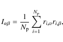
$\begin{displaymath}I_{\alpha \beta}= \frac{1}{N_{\rm p}} \sum_{i=1}^{N_{\rm p}} {r_{i, \alpha} r_{i, \beta}} , \end{displaymath}$

(4)

where the positions r_i are given with respect to the centre of mass and the summation is over all particles in the halo ( $N_{\rm p}$ ). The axes of the ellipsoid can be determined from the eigenvalues $\lambda_{i}$ of the inertia tensor as $a= \sqrt{\lambda_1}$ , $b= \sqrt{\lambda_2}$ , $c= \sqrt{\lambda_3}$ , where $a \ge b \ge c$ . Haloes can be classified in terms of their axis ratios by defining their degree of sphericity s, prolateness q, and oblateness p as

$\begin{displaymath}s=\frac{c}{a}; p=\frac{c}{b}; q=\frac{b}{a}\cdot \end{displaymath}$

(5)

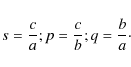
An additional measure for the shape of the ellipsoid is the triaxiality parameter (Franx et al. 1991),

$\begin{displaymath}T=\frac{a^2-b^2}{a^2-c^2} \cdot \end{displaymath}$

(6)

An ellipsoid is considered oblate if 0<T<1/3, triaxial with 1/3<T<2/3, and prolate if 2/3<T<1.

4 Testing the halo finder

Before using the ASOHF finder in real cosmological applications, we have to be sure that it provides accurate and credible results. In order to validate and assess the robustness of our method, we developed a set of tests that will allow us to quantify the uncertainty of the halo finder algorithm and to check the properties of the haloes found with it.

In these tests we build mock distributions of dark matter particles, made by hand, resembling real outputs of cosmological simulations. Therefore, we have perfectly known distributions of dark matter particles forming a given number of cosmological structures with physical parameters completely known. Once these distributions are built, we apply the halo finder and compare the results obtained with the ones originally adopted to create the mock distributions by hand.

The different numerical implementations presented in this section were performed assuming the following cosmological parameters: matter density parameter, $\Omega_{\rm m}=0.25$ ; cosmological constant, $\Omega_{\Lambda}=\Lambda/{3H_0^2}=0.75$ ; baryon density parameter, $\Omega_{\rm b}=0.045$ ; reduced Hubble constant, h=H₀/100 km s^-1 Mpc ^-1=0.73; power spectrum index, $n_{\rm s}=1$ ; and power spectrum normalization, $\sigma_8=0.8$ .

The set of tests was designed to help us check different aspects of interest in cosmological simulations: i) test 1 and test 2 are focussed in looking for and characterizing single haloes and subhaloes, respectively; ii) test 3 builds the merger trees of haloes; and iii) test 4 analyses big samples of haloes.

All cases considered in this section were placed in a comoving volume of 100 h^-1 Mpc on a side. The computational box has been discretised with 256³ cubical cells. All our modelled haloes will be spherical, with a given dark matter density profile, mass, and radius. From now on, these artificial or modelled haloes will be called template haloes.

Depending on the test we are analysing, we need to define the number of template haloes we want to study, the number of time outputs (different redshifts we look at), as well as the total number of dark matter particles to be used. The total number of particles must be conserved during the whole evolution to guarantee mass conservation, and it must be chosen as a compromise between having a good resolution in mass for each halo and the computational cost. In the particular implementation of all tests presented in this section we assumed for simplicity's sake, equal mass dark matter particles with masses $m_{\rm p} \simeq 5.0 \times10^{9}~M_\odot$ .

4.1 Test 1: looking for single haloes

The first test presented is designed to check the ability of the halo finder to look for single haloes and compute their main physical properties at a given redshift: position, mass, and radius. To achieve this we generate an artificial sample of haloes with different numbers of dark matter particles, and with positions, virial radii, and virial masses fixed by hand. Then the halo finder is applied to this mock universe to verify whether the detected haloes agree with those previously made by hand.

Table 1: Mean features of the generated haloes at z=0 in test 1.

Let us describe the method to generate these artificial haloes. Assuming some general features (cosmological parameters, number of time steps, number of desired haloes and total number of particles), the properties of the haloes that populate each time step are made by hand: the number of dark matter particles within each halo (and hence, their masses) and the coordinates of their centres. With this information and the cosmological parameters the average density corresponding to a given epoch as well as the virial radius from Eq. (2) of the haloes are computed. Once the main physical properties of the haloes have been defined, each halo is created by a random distribution of dark matter particles - using the rejection sampling method (von Neumann 1951) -, in a way that its density profile is consistent with a NFW profile (Navarro et al. 1997).

In this subsection we present a case characterized by the usual cosmological parameters and with $\sim$ 10⁵ dark matter particles in a unique time step corresponding to z=0. For this test we generated four dark matter haloes with density profiles compatible with NFW, in the way explained before. The main properties of these mock haloes are summarized in Table 1.

$\begin{figure} \par\includegraphics[width=12.2cm]{14214fg2.ps} \end{figure}$	Figure 2: Radial dark matter density profiles for the four generated haloes compiled in Table 1 as a function of the radius at z=0 (test 1). Continuous lines stand for the input profiles of the mock haloes, whilst points represent the profiles obtained by the halo finder.
Open with DEXTER

The ASOHF halo finder was applied to this mock simulation. The mean relative errors found in the computation of the positions and radii are of the order of $0.1\%$ . The masses are perfectly recovered because all particles forming the halo are identified. Note that although the results seem excellent, they correspond to an extremely idealised test.

In Fig. 2 we plot the radial density profiles used as input to generate - using the rejection method - the haloes (continuous line) and the obtained profiles (dots). These last profiles were computed by averaging the dark matter density in spherical shells of a fixed logarithmic width.

We fitted a NFW density profile to each one of the obtained profiles. The concentration, inner and outer slopes are shown in Table 1, respectively. In Col. 7 of this Table, we present the concentration obtained from the fitting together with the concentration of the density profile used as input (between parenthesis). For the inner (outer) slope of the density profile that we denoted by $\alpha$ ( $\beta$ ), the fitted value must be compared with 1.0 (2.0), which corresponds to the value adopted in the input profile.

We checked that the errors encountered for the fitted profiles are mostly caused by the rejection sampling method. In this line we tested that the sampling of an input density profile with the rejection method produces particle distributions that trace the underlying density profile with a precision of a few per cent. Therefore, when the halo finder finds a halo and obtains its density profile, there is also a small error when compared with the input density profile. But it must be kept in mind that this error does not arise from the halo finder algorithm itself but from the way that this particular test has been set up.

Although this test is very simple, because it only considers four haloes in a single time step, it provides us with a powerful tool to verify the behaviour of our finder in a very basic situation. We checked many other configurations (some of them really unrealistic) with similar results. Due to its clarity and simplicity we have chosen this one to demonstrate our objective.

4.2 Test 2: looking for subhaloes

$\begin{figure} \par\includegraphics[width=15.5cm]{14214fg3.ps} \end{figure}$

Figure 3:

Mock distribution of a halo with three substructures: two subhaloes and one sub-subhalo (test 2). The left panel shows the 2D projection of the structures found by ASOHF. Circles represent the radii of the different structures, while the different line types stand for the different refinement levels in which the haloes have been found. The right panel shows the known distribution of dark matter particles in this test. Different colours stand for the level to which the particles belong.

Open with DEXTER

In this section we present a simple test that was designed to check the ability of ASOHF to deal with substructures.

Following the idea of test 1, we generated by hand a simple distribution of haloes placed in different levels of resolution of a very basic AMR grid similar to that of the MASCLET code. For the sake of simplicity, only three levels of refinement (the ground grid and two upper levels) were considered. The hierarchy of structures and substructures generated for this test are distributed according to these levels.

Among all configurations that we tried for this test, we chose because of its clarity a simple one in which four structures are considered: a big dark matter halo in the coarse level hosting two subhaloes where at the same time one of these subhaloes hosts a smaller subhalo, which is a sub-subhalo of the big one.

Figure 3 shows the configuration analysed in this test. A visual inspection of this plot shows that the halo finder also works properly when dealing with substructures located in different levels of an AMR grid.

Additionally, the mean relative errors given by ASOHF in the estimation of the main properties of the generated structures are of the order of $3\%$ , $0.1\%$ and $1\%$ for the mass, position, and radius, respectively. This value together with a visual inspection of Fig. 3 is an excellent indicator of the good performance of ASOHF when working with structures that contain different substructures, at least in a simple configuration like the one considered here.

Because this configuration is very basic, we check this situation in Sect. 5 for a proper cosmological simulation and compare the results obtained by ASOHF with those obtained by other well known halo finders.

4.3 Test 3: testing the merger tree

Once we checked that the ASOHF finder works properly when it looks for single haloes and subhaloes, we checked how well it computes the merger tree for each.

In this section we consider several configurations characterized by the same parameters as in the previous ones, but with more than one time step. Now the idea is to generate a given number of haloes, in the simple way explained before, but forcing different time evolutions of these haloes.

We are interested in studying the most common events in the evolution of dark matter haloes: i) relaxed or isolated evolution, i.e., without important interactions or mergers with other haloes (case I); ii) ruptures or disruptions of a single halo into two or more smaller haloes owing mainly to interactions with the environment or with other haloes (case II); and iii) mergers between two or more haloes (case III). To do this we chose four haloes at a given redshift which are those compiled in Table 1, and studied their evolution in the three different cases that have into account in a simple way the most common events explained before. Then, ASOHF is applied to these artificial evolutions to compare the obtained merger trees with the generated ones.

Again, for the sake of simplicity and brevity, a reduced number of haloes will be considered, but note that more complicated configurations were studied and can be easily implemented.

Figure 4 shows the merger trees obtained by ASOHF in the different cases considered here. The top panel of Fig. 4 shows the complete merger tree obtained for the four haloes studied in each of the three cases presented here. In the bottom panel of the same figure, the same cases are represented but following only the closest particle to the centre of each halo (reduced merger tree).

The line segments joining the circles in Fig. 4 are a relevant feature of the plot because they indicate that the halo at the earlier time is considered to merge into (or to be identical to) the halo at the later time. Moreover, in the upper panel the different line types represent the percentage of mass that goes from one halo to another. Thus, a halo at later time connected with a halo at earlier time by a dash-dotted line means that up to 25% of its total mass comes from that halo at earlier time. The same idea applies to the other line types.

The horizontal axis is designed to separate the haloes according to their future merging activity. It does not directly indicate space positions, although there should be some correlation between how close two haloes are in the plot and how close they are in space (because haloes need to be close to merge later on). The vertical axis shows the redshift of each time step in the simulation. The size of each circle indicates the virial mass of each halo normalized to its final mass at the last iteration. Because the iterations go in descending order, the last iteration corresponds to the lowest redshift.

The different cases analysed in this section and their representation in Fig. 4 are discussed in detail in the subsections below.

$\begin{figure} \par\includegraphics[height=14cm]{14214fg4.ps} \end{figure}$

Figure 4:

Merger trees for several haloes in the three different cases analysed in Sect. 4.3 (test 3). Left, central, and right panels stand for case I, II, and III, respectively. The top panels represent the results obtained following all dark matter particles within each halo (complete merger tree), whereas the bottom panels stand for the results obtained following only the closest particle to the centre of each halo (reduced merger tree). Haloes are represented by circles whose sizes are normalized to the final mass at z=0. The different line types connecting haloes at different times in the upper plots indicate the amount of mass transferred from the progenitors to their descendants.

Open with DEXTER

4.3.1 Case I

In this first case, we study the most trivial situation. Only two time steps corresponding to $z \sim 0.5$ and $z \sim 0.3$ are considered. The objective is that the four haloes generated at $z \sim 0.5$ would be exactly the same as those at $z \sim 0.3$ . The selection of the redshifts is made in order to obtain a fast evolution of the haloes, but it is possible to make it for time steps much more realistic and separated in time. In any case, this selection is not relevant to achieve our objective, which is to check the performance of the halo finder computing the merger tree of a given halo, i.e., following the particles that belong to a halo at a given epoch through the evolution.

The haloes at different epochs are generated in the way explained above. In this particular case, we force that the four considered haloes at both epochs would be identical, i.e., with the same particles in each one and with the same radius and position of the centre.

In order to be as clear as possible when talking about haloes at different epochs, we will use the notation h_ij, where istands for the iteration number (iterations in descendant order and then corresponding the iteration or time step 1 to the lowest redshift) and j for the halo number in the iteration i, respectively.

According to this notation, the generated relations between the haloes in this case are

$\bullet$: $h_{21} \Longrightarrow h_{11} [100\%]$
$\bullet$: $h_{22} \Longrightarrow h_{12} [100\%]$
$\bullet$: $h_{23} \Longrightarrow h_{13} [100\%]$
$\bullet$: $h_{24} \Longrightarrow h_{14} [100\%]$ .

These connections tell us we are working only with two time steps (2 corresponding to $z \sim 0.5$ and 1 to $z \sim 0.3$ , respectively) and each one of these epochs has four haloes (j runs from 1 to 4 in both time steps). In addition, the number between square brackets informs us about the percentage of the mass of each halo that it obtains from its progenitor. For instance, the first relation tells us that the $100 \%$ of the mass of the halo number one in the last iteration (h₁₁) comes totally ( $100 \%$ ) from the halo number one in the previous time step (h₂₁).

We applied the halo finder to this artificial evolution and constructed the merger tree of the selected haloes tracking all dark matter particles for a given halo backwards in time. For each halo in this case, two merger trees, the complete and the reduced one, have been built. The left panels of Fig. 4 show the obtained results. The upper-left plot of this figure shows the complete merger tree for the considered haloes, whereas the lower-left plot represents the reduced merger tree for the same haloes.

According to these plots it is evident that for case I the halo finder tracks the correct history for all considered haloes.

Additionally, the connection lines linking the haloes at different redshifts in the complete merger tree inform us about the percentage of mass that each younger halo receives from its progenitors. In this particular case, this percentage is in all cases greater than $75\%$ , in perfect agreement with the expected results ( $100 \%$ ). More precisely, the obtained results are

$\bullet$: $h_{21} \Longrightarrow h_{11} [99.97\%]$
$\bullet$: $h_{22} \Longrightarrow h_{12} [99.98\%]$
$\bullet$: $h_{23} \Longrightarrow h_{13} [99.99\%]$
$\bullet$: $h_{24} \Longrightarrow h_{14} [99.99\%]$ .

Although in this example the obtained percentages are very accurate with regard to the expected ones, we should point out that they are not always exact. This is because although the particles are forced to be the same and belong to a given halo, they are distributed randomly. Thus, the haloes are not exactly found within the same boundaries by the finder for different redshifts in this test and then some particles are not taken into account.

4.3.2 Case II

In this case we are interested in checking the capabilities of the halo finder when some haloes suffer one or several disruptions during their evolution, when they lose mass and reduce their size. This process operates at two regimes for different reasons. This is quite common in very small size haloes. The reason is that these haloes are not really gravitationally well bound and can easily be disrupted by interactions with environment or with other haloes. For larger haloes, those mass losses are smaller and they are usually associated with tidal interactions.

To study this case we started at $z \sim 0.5$ with the four haloes summarized in Table 1. Now, three time steps of the haloes evolution corresponding to $z \sim 0.5$ , $z \sim 0.3$ and z=0 are considered. The results of this situation are shown in the middle panels (top and bottom) of Fig. 4.

Here the generated evolutions can be summarized in the following relations. In a first step, the connections between the haloes of the third ( $z \sim 0.5$ ) and the second ( $z \sim 0.3$ ) iterations are

$\bullet$: $h_{31} \Longrightarrow h_{21} [100\%]$
$\bullet$: $h_{32} \Longrightarrow h_{22} [100\%] , h_{23} [100\%]$
$\bullet$: $h_{33} \Longrightarrow h_{24} [100\%]$
$\bullet$: $h_{34} \Longrightarrow h_{25} [100\%]$ .

On the other hand, the links between the haloes generated in the second iteration ( $z \sim 0.3$ ) with those in the first one (z=0) are

$\bullet$: $h_{21} \Longrightarrow h_{12} [100\%] , h_{14} [100\%]$
$\bullet$: $h_{22} \Longrightarrow h_{11} [100\%]$
$\bullet$: $h_{23} \Longrightarrow h_{13} [100\%]$
$\bullet$: $h_{24} \Longrightarrow h_{16} [100\%] , h_{18} [100\%]$
$\bullet$: $h_{25} \Longrightarrow h_{15} [100\%] , h_{17} [100\%]$ .

As a result of the whole evolution there are eight haloes instead of the first four, which were generated in the same manner as in the previous case, but which were forced to share a certain number of particles with their ancestors, which property is the key to build their evolution history.

After building these artificial evolutions, ASOHF was applied to this mock universe to obtain the merger trees of the involved haloes.

As we can see in the upper-middle plot (case II) of Fig. 4, the halo finder again provides very accurate results, in perfect agreement with those exposed before. In all cases the obtained percentages are between $99.9\%$ and $100 \%$ . Again, the value of the percentages can be explained if we take into account that each halo has been populated with particles randomly placed. Then, the particles positions are not always the same and small deviations are expected.

If we compare the upper-middle plot of Fig. 4 (complete merger tree) with the lower-middle plot (reduced merger tree), the results completely agree but in the lower plot each halo is only allowed to have one descendant at maximum.

4.3.3 Case III

Here the response of the halo finder in a merger between two or more haloes is checked.

To analyse this, we started again with the same haloes and time steps as before. Now, the different evolutions can be summarized with the following links. In a first step the connections between the haloes of the third ( $z \sim 0.5$ ) and the second ( $z \sim 0.3$ ) iterations are (the same as in the previous case)

$\bullet$: $h_{31} \Longrightarrow h_{21} [100\%]$
$\bullet$: $h_{32} \Longrightarrow h_{22} [100\%] , h_{23} [100\%]$
$\bullet$: $h_{33} \Longrightarrow h_{24} [100\%]$
$\bullet$: $h_{34} \Longrightarrow h_{25} [100\%]$ .

But now the links between the haloes of the second ( $z \sim 0.3$ ) and first (z=0) iterations are

$\bullet$: $h_{21}+h_{24}+h_{25} \Longrightarrow h_{12} [74.49\% + 9.48\% + 16.03\%]$
$\bullet$: $h_{22} \Longrightarrow h_{11} [100\%]$
$\bullet$: $h_{23} \Longrightarrow h_{13} [100\%]$ .

In the end three haloes are obtained as a result of the different processes that happened during their evolution.

From the right panels of Fig. 4 (top and bottom plots), we can deduce that despite the triple merger that has taken place in the last time step, the halo finder provides very accurate results. Indeed, the results obtained for this merger event are

$\bullet$: $h_{21}+h_{24}+h_{25} \Longrightarrow h_{12} [74.45\% + 9.45\% + 16.08\%]$ ,

where the percentages perfectly agree with the expected ones.

4.4 Test 4: analysing a sample of haloes

$\begin{figure} \par\includegraphics[height=10cm]{14214fg5.ps} \end{figure}$	Figure 5: Top panel: academic mass function corresponding to the generated sample of 100 haloes for test 4. Dots represent the mass function obtained by ASOHF, whereas the continuous line corresponds to the function generated by hand. Bottom panel: relative error or difference in mass between the two distributions shown in the upper plot.
Open with DEXTER

The analysis of big samples of haloes is crucial in cosmological applications. Therefore, once we checked the halo finder works correctly looking for single haloes and constructing their merger trees, we should check what its response is when working with a large sample of haloes and computing all their properties. Once this sample of haloes is built, an academic mass function, i.e., the mass distribution of all the generated haloes, is computed.

For the sake of simplicity, only one time step corresponding to z=0 was considered. Then a sample of 100 haloes with masses randomly distributed between $1.0 \times10^{13}~ M_\odot$ and $1.0\times10^{15}~ M_\odot$ , was generated. The position of the centre and the radius of each halo are obtained randomly, whereas the number of particles belonging to each one of them is derived from their masses.

Once this mock universe was generated, the ASOHF finder was applied. Then the academic mass function of the well known distribution of haloes is compared with the mass function of the sample of haloes obtained by ASOHF.

The results obtained in this case are shown in Fig. 5, in which the number of objects of a given mass is plotted as a function of the mass. This plot shows the theoretical or academic mass function (continuous line) and the one obtained by ASOHF (filled dots). As we can see, these two distributions are almost completely superposed. As a proof of the precision of the finder we can compare the masses of the most and less massive haloes of the sample obtained by the two methods. Thus, the most massive halo found by the finder has a mass of $9.8622 \times10^{14}~M_\odot$ , whereas this halo was supposed to have a mass of $9.8623 \times10^{14}~M_\odot$ . The same occurs for the less massive halo, which was found by the finder to have a mass of $1.48 \times10^{13}~M_\odot$ , whereas it was supposed to have a mass of $1.49 \times10^{13}~M_\odot$ . In addition, as we can see in the bottom panel of Fig. 5, the maximum value of the relative error in mass between the theoretical and the obtained mass functions is $\sim$ $5\%$ .

5 Comparison with other halo finders

In this section we compare the results of ASOHF with two other halo-finding mechanisms, namely AFoF (van Kampen 1995) and AHF (Knollmann & Knebe 2009). We applied these three halo finders to a cosmological simulation carried out with the cosmological code MASCLET. The main properties of this simulation are explained below.

For the AFoF run, a linking length of 0.16 times the mean DM particle separation was used, yielding an overdensity at the outer radius comparable to the virial overdensity used in the ASOHF run. This linking length is obtained when scaling the standard linking length of 0.2 by $(\Delta_{\rm c}/ \Omega)^{-1/3}$ according to the adopted cosmology (Eke et al. 1996).

For the run with AHF, we used a value of 5 for the parameters with regard to the refinement criterion on the domain grid (DomRef) and on the refined grid (RefRef), respectively. To understand the role of these parameters we need to explain briefly how AHF operates. Once the user has provided the particle distribution, the first step in AHF consists in covering the whole simulation box with a regular grid of a user-supplied size. In each cell the particle density is calculated by means of a triangular shaped cloud (TSC) weighting scheme (Hockney & Eastwood 1988). If the particle density exceeds a given threshold (the refinement criterion on the domain grid, DomRef), the cell is refined and covered with a finer grid with half the cell size. On the finer grid (where it exists), the particle density is recalculated in every cell and then each cell exceeding another given threshold (the refinement criterion on refined grids, RefRef) is refined again. This is repeated until a grid is reached on which no further cell needs to be refined. Following this procedure yields a grid hierarchy constructed in a way that it traces the density field and can then be used to find haloes and subhaloes in a similar way to that used by ASOHF.

In all the runs, an equal minimum number of dark matter particles per halo was considered. This number has been set to 50 particles per halo. In spite of this consideration, we expect some differences in the final results obtained with the different halo finders. The main explanation for these expected discrepancies has to do with the different techniques used by the three methods in the generation of the density field and hence in the definition of the haloes. However, general properties of the simulation should be well described by the three finders.

5.1 Simulation details

The simulation described here was performed with the cosmological code MASCLET (Quilis 2004). This code couples an Eulerian approach based on high-resolution shock capturing techniques for describing the gaseous component with a multigrid particle mesh N-body scheme for evolving the collisionless component (dark matter). Gas and dark matter are coupled by the gravity solver. Both schemes benefit by using an AMR strategy, which permits them to gain spatial and temporal resolution.

The numerical simulation was performed assuming a spatially flat $\Lambda$ CDM cosmology with the following cosmological parameters: matter density parameter, $\Omega_{\rm m}=0.25$ ; cosmological constant, $\Omega_{\Lambda}=\Lambda/{3H_0^2}=0.75$ ; baryon density parameter, $\Omega_{\rm b}=0.045$ ; reduced Hubble constant, h=H₀/100 km s^-1 Mpc ^-1=0.73; power spectrum index, $n_{\rm s}=1$ ; and power spectrum normalization, $\sigma_8=0.8$ . The initial conditions were set up at z=50, using a CDM transfer function from Eisenstein & Hu (1998) for a cube of a comoving side length 47 h^-1 Mpc. The computational domain was discretised with 256³ cubical cells.

This simulation uses a maximum of six levels of refinement, which gives a peak spatial resolution of 3 h^-1 kpc. For the dark matter two particles species were considered to be the best mass resolution $\sim$ $4\times 10^7~ h^{-1}~ M_\odot$ , equivalent to distribute 256³ particles in the whole box.

Table 2: General results obtained by ASOHF, AFoF and AHF at z=0.

$\begin{figure} \par\includegraphics[height=100mm]{14214fg6.ps} \end{figure}$	Figure 6: Top panel: comparison of the mass functions obtained by ASOHF, AHF and AFoF at z=0. The mass function predicted by Sheth & Tormen is also shown. Bottom panel: relative difference in the number of haloes between AFoF and AHF compared to ASOHF.
Open with DEXTER

5.2 Halo mass function

$\begin{figure} \par\includegraphics[height=90mm]{14214fg7.ps} \end{figure}$	Figure 7: 2D projection for haloes at z=0. Only haloes with masses above $1.0\times10^{12}~M_\odot h^{-1}$ are shown. Left panel stands for haloes and subhaloes found by ASOHF, whereas right panel corresponds to those found by AHF. The size of the different haloes is given by their virial radii.
Open with DEXTER

Here we present the sample of haloes obtained from the cosmological simulation by the three halo finders used in the present study, namely ASOHF, AFOF and AHF. Their main properties and differences are discussed.

The three halo finders obtained a relatively large sample of galaxy clusters and groups spanning an approximated range of masses from $1.0 \times10^{9}~M_\odot ~ h^{-1}$ to $2.0\times10^{14}~M_\odot ~h^{-1}$ . The total number of structures identified by ASOHF, AFoF, and AHF has been 1339, 7448, and 1712, respectively. Although the numbers and masses of the detected haloes are roughly consistent, they are, as expected, slightly different among them. These results are more similar between ASOHF and AHF, whereas AFoF identifies more smaller haloes.

To analyse the simulation mass function, we restricted ourselves to study the best-resolved haloes, that is those haloes with masses above $1.0\times10^{12}~M_\odot ~h^{-1}$ . The number of haloes with masses above this limit and the maximum and minimum masses (in all the sample) of the found haloes by the different halo finders are summarized in Table 2. The obtained results by the three finders, although very similar, are not exactly the same. This was expected because each halo finder uses different approximations and techniques. ASOHF uses the grid hierarchy generated by the cosmological simulation itself, whereas AHF has to construct a new set of grids with different criteria because only a list of particles is provided to them which is consequently not identical with that used by ASOHF.

In Fig. 6 we compare the mass functions at z=0 of the simulation as obtained by the different halo finders in this study. We also present a comparison with the mass function proposed by Sheth & Tormen (1999) (ST).

$\begin{figure} \par\includegraphics[height=150mm]{14214fg8.ps} \end{figure}$

Figure 8:

Distribution of the halo shapes at z=0 as found by ASOHF ( left panels) and AHF ( right panels), respectively. Only haloes with masses above $1.0\times10^{12}~M_\odot h^{-1}$ are taken into account. The top plots show the distribution of p=c/b against q=b/a. The dashed line represents the division between oblate and prolate haloes. The shaded grid was computed by binning individual haloes to a two-dimensional grid. Six contour lines equally spaced are plotted to highlight the shape of the two-dimensional distributions. The bottom panels show the triaxiality parameter as a function of the halo masses. The error bars represent $\sqrt N$ uncertainties due to the number counts in the different mass bins.

Open with DEXTER

The obtained mass functions show a considerable dispersion mainly in the lower limit of mass compared with the ST prediction. Note though that the theoretical mass function proposed by ST has been calibrated using an overdensity of $\Delta_{\rm c}=174$ (Tormen 1998), whereas in our case this overdensity is $\sim$ 374. The bottom panel of Fig. 6 displays the relative deviation of the mass functions obtained by AFoF and AHF with respect to the results produced by ASOHF. Hence, a positive deviation means that the ASOHF run found more haloes in the given bin than the halo finder it is compared with. Generally speaking, we find good agreement between the three mass functions, although ASOHF and AHF results exhibit a better resemblance, which is expected because the similarities of both methods.

Let us point out that the dispersion of the mass function when compared with the reference mass function (ST) is a well known issue. We stress that is out of the scope of this paper to discuss how representative the considered simulation is. Instead, we use this simulation to test whether the different halo finders produce similar results. In this sense, we emphasize that the three algorithms compared agree very well.

For the sake of completeness, we mention that the dispersion of the mass function is a complex topic that is abundantly discussed in the literature. A few examples, among many others, could be: i) the work by Reed et al. (2007), where the authors study the dispersion of the mass function for several simulations depending on the redshift; ii) the results of the GIMIC project (Crain et al. 2009), where an important dispersion in the mass function is shown depending on the considered region; and iii) the dispersion of the mass function found by Yaryura et al. (2010) related with very large structures.

From now on, we restrict ourselves to analyse only the main differences between the AHF and the ASOHF codes, that is, between the ``grid based on halo finders''. The reason is that these methods are more directly comparable with each other. Still, given that we use AHF as a stand-alone halo finder, differences are expected.

To have a first order comparison of the spatial distribution of the haloes encountered by both codes, Fig. 7 shows the 2D projection along the z axis of the simulated box of all haloes (and/or subhaloes) found by ASOHF and by AHF at z=0. We only show those haloes or subhaloes with masses larger than $1.0\times10^{12}~M_\odot ~h^{-1}$ . Both panels are highly consistent. All relevant features of the halo distribution were caught with both methods, and therefore they seem perfectly comparable.

The main differences between both methods arise when the smallest structures found are taken into account. Whereas the biggest structures are perfectly recognized in both plots, the smallest represent the main source of disagreement. These discrepancies may have a variety of causes, of which the most important is that the finders make use of very different techniques to compute the dark matter density distributions. Both codes create their structures of nested grids according to different criteria. Therefore, a slight change in the number of grids, especially for the small objects, could alter the way in which these objects are resolved, making them detectable or not. Leaving this issue aside, both distributions are fully comparable.

5.3 Halo shapes

The shapes of haloes are described by the axes, $a \ge b \ge c$ , of the ellipsoid derived from the inertia tensor, as described in Sect. 3.3. For the sake of completeness, we have compared the distribution of halo shapes obtained by ASOHF and AHF for haloes with masses above $1.0\times10^{12}~M_\odot ~h^{-1}$ . The obtained results are shown in Fig. 8. As we can deduce from these results, haloes are generally triaxial but with a large variation in shapes. Prolate objects have p=1, oblate objects have q=1, and spherical objects have p=q=1.

Our results show that the haloes are mainly spherical but with a slight preference for prolateness over oblateness. This distribution qualitatively agrees with previous results (e.g., Cole & Lacey 1996; Frenk et al. 1988; Bailin & Steinmetz 2005).

$\begin{figure} \par\includegraphics[height=130mm]{14214fg11} \end{figure}$	Figure 9: Merger tree of the analysed host halo. Cluster haloes are represented by circles whose sizes are normalized to the final mass at z = 0. Lines connecting haloes at different times indicate the amount of mass transferred from the progenitors to their descendants. Only the contribution of the most massive progenitors is displayed.
Open with DEXTER

Bottom panels of Fig. 8 show the triaxiallity parameter, T, of the haloes found by ASOHF (left plot) and AHF (right plot) as a function of halo masses. In this figure the x-axis was divided into 12 mass bins equally spaced in logarithmic scale, and the error bars represent $\sqrt N$ uncertainties due to the number counts. The general trends obtained from these plots agree with previous results (e.g., Shaw et al. 2006; Allgood et al. 2006; Warren et al. 1992). As it would be naively expected, more massive haloes tend to be less spherical and more prolate. In a hierarchical model of structure formation, more massive haloes form later, and have less time to relax and to form more spherical configurations. In addition, because haloes tend to be formed by matter collapsing along filaments, they generally lead to prolate rather than oblate structures. Because our halo sample is statistically small, the general trend obtained for the shape of the haloes must be taken with caution although it agrees with previous results. Nevertheless, even when the sample can be limited, results from ASOHF and AHF are completely consistent.

5.4 Subhaloes

One of the main features of the ASOHF finder is its capacity to deal with haloes and subhaloes. In this section we compare the abundance and distribution of substructures given by ASOHF and AHF.

For the sake of comparison, we focus on the detailed analysis of the most massive halo in the cosmological simulation previously described. This halo has a virial mass of $\sim$ $8.0 \times10^{14}~ M_\odot$ and a virial radius of $\sim$ 2.4 Mpc. To illustrate the time evolution of the chosen halo, we constructed its merger tree by tracking all its particles backwards in time. In Fig. 9 we display the merging history of the halo. To facilitate the reading of this figure, we only show the mergers among the most massive haloes that contribute to build up the final halo at z=0. Otherwise, the plot would be saturated by the amount of mergers due to small structures, which are not very relevant from the dynamical point of view, though. The merger tree starts at z=0 and it plots all the most massive progenitors of the final halo in previous time-steps over several output times of the simulation. The total mass of each halo is represented by a circle, whose size is normalized to the mass of the final halo at z=0. The meaning of the different line types remains the same as in Sect. 4.3 (Fig. 4), that is the amount of mass received by any of the progenitors. This kind of plot not only shows the merger history, but also the different interconnections over time. Although this halo is the most massive in the simulation, it is far from being virialized because, as we can see in Fig. 9, it has suffered several major mergers during its evolution, one of which happened very recently. This makes the process of the substructure analysis more challenging.

In Fig. 10 we present the analysis of this particular halo with its substructures as found by ASOHF (upper plots) and AHF (lower plots), respectively. The left column of the panel displays the 2D projection of the halo with its subhaloes. The x and y axes show the coordinates in Mpc of the haloes within the computational box. The comparison of the haloes identified by both codes deserves some comments. The main halo is located at the same coordinates and with the same mass and size in both cases. There is also a clear correlation among the largest subhaloes in both subhalo samples in sizes and masses. But there seem to be important differences in the smallest substructures. As we mentioned above, the explanation of this different performance detecting small structures is directly linked with the structure of nested grids built by the algorithms.

Subhalo mass functions have been widely studied in previous works (e.g., De Lucia et al. 2004; Giocoli et al. 2008a; Knollmann & Knebe 2009; Gao et al. 2004; Ghigna et al. 2000), leading to the conclusion that subhalo mass functions can be described with a power law, $N_{\rm sub} (>$ $M) \propto M^{- \alpha}$ , with a logarithmic slope $\alpha$ in the range from 0.7 to 0.9. We computed the subhalo mass function of the cosmological simulation used for the comparison of both halo finders. The results are shown in the panels of the right column in Fig. 10. These plots show the cumulative mass functions of the subhaloes for the considered main halo as obtained by ASOHF (top) and AHF (bottom). To facilitate the comparison with previous results, two lines corresponding to the power laws with values of $\alpha$ equal to -0.7 and -0.9 are plotted. The masses of subhaloes are normalized to the mass of the main halo. The error bars show $\sqrt N$ uncertainties due to the number counts.

$\begin{figure} \includegraphics[height=160mm] {14214fg9.ps} \vspace*{0.25mm} \end{figure}$

Figure 10:

Analysis of the subhalo population of the most massive halo in our simulation. Left panels (top and bottom plots): subhalo population within the most massive host halo in our simulation as found by ASOHF and AHF. The size of the circles represents the virial radius of the different haloes. Right panels: cumulative subhalo mass function for the most massive halo in our simulation as found by ASOHF (upper plot) and AHF (lower plot). Two power law fits with slopes of -0.7 and -0.9 are also shown in these panels. Error bars show $\sqrt N$ uncertainties due to the number counts.

Open with DEXTER

$\begin{figure} \includegraphics[height=85mm]{14214fg10} \end{figure}$	Figure 11: 2D projection of the dark matter density field around the biggest halo in the simulation. The colour scale represents the logarithmic of the density field. Subhaloes found by ASOHF (left panel) and AHF (right panel) are superimposed being the white circles the radii of these haloes.
Open with DEXTER

From a statistical point of view, the comparison of both mass functions shows that both codes have similar capabilities when dealing with finding substructures. The fitting to a power law of the analysed data gives a slope of 0.9 for ASOHF and 0.7 for AHF. This would render the ASOHF and AHF mass functions completely consistent with previous results, because they are well fit between the two limiting power laws for substructure in haloes. Nevertheless, this conclusion must be taken with caution because, as we saw, a direct comparison of the smallest substructures is not straightforward.

We proceed to compare identified subhaloes with the real mass distribution in the main halo to deepen in the comparison of the encountered subhalo samples and assuming that a direct comparison between both methods is not always completely meaningful. Therefore, Fig. 11 shows the colour-coded dark matter column density in the main halo considered in this section together with the detected subhaloes overplotted as circles with their radii normalized to the main halo radius. The left panel of the figure corresponds to the sample obtained by ASOHF, whereas the right panel displays subhaloes identified by AHF. As we previously discussed when analysing Fig. 10, most of the substructures are unambiguously identified by both codes and with very similar features (sizes and masses). However, the smallest subhaloes are not well identified either with ASOHF or AHF. Moreover, it is striking that some of these small substructures do not match not only between both halo finders, but more intriguing, with the real mass distribution.

6 Summary and conclusions

In the last years cosmological simulations have experienced an astonishing development, producing a huge amount of computational data. Intimately related to the development of simulations, all kinds of analysis tools have arisen too. One of the most important analysis tools have become the halo finder algorithms, whose relevance is crucial when comparing simulations with observation.

The halo-finding issue has revealed itself as not trivial at all. When cosmological simulations have increased their resolution and complexity and the amount of data have grown exponentially, to find haloes can itself be an intensive computational work. Moreover, the different techniques and implementations used in the halo finders developed so far can show important differences, particularly when looking at the features of the smallest objects in the simulations.

We developed a new halo-finding code with the main idea of contributing towards constraints for a field in which only a limited number of algorithms are available and differences among codes are still relevant.

Our ASOHF code was especially designed to overcome some limitations of the original SO technique and to exploit the benefits of having a set of nested grids that track the density distribution in the analysed volume. By treating all AMR grids at a certain level of refinement (same numerical resolution) independently, the code is able to find haloes at all levels. This procedure can identify haloes in haloes in a natural way and therefore describe the properties of the substructure in cosmological objects.

The numerical scheme is also prepared to compute the merger tree of the haloes in the computational box as well as some other usual properties of these haloes such as their shapes, and density and velocity radial profiles.

We set up several idealised and controlled tests to check the capabilities of the halo finder. Although most of these tests are unreal, they allow us total control of every part of the halo-finding process. In all tests, the performance of the finder algorithm has been correct.

The next step to calibrate and test the ASOHF finder was to apply it to the outcome of a cosmological simulation and compare its results with other halo finders widely used like AHF and AFoF.

In a first instance, we compared the sample of haloes encountered by the three codes in a given cosmological simulation. A coarse comparison showed a good agreement among them. The mass functions obtained by the three finders were also very similar. We looked at the shape of the encountered haloes, finding a reasonable concordance between the results obtained by ASOHF and AHF and with previous studies.

More interestingly, we tested the abilities of ASOHF dealing with substructure in not idealised simulations. In order to check this issue, we picked up the most massive halo in the considered computational box. This halo was throughly analysed using both grid based on finders, namely, ASOHF and AHF. From the statistical point of view, the results are comparable because the subhalo mass functions are reasonably consistent. Still, the comparison object by object was not as successful because there are several noticeable differences concerning the smaller objects. To clarify this, we compared the samples of haloes obtained by both algorithms with the real mass distribution. Apparently, both codes agree among themselves and match the mass distribution for the most relevant features. However, both algorithms miss small objects when they are compared with the mass distribution. Surprisingly, the two codes do not miss the same small objects.

The explanation for this behaviour for the ASOHF finder is related to how the hierarchy of nested grids is created. We checked that some of those smaller objects are not always covered by a high resolution grid. In that case the halo finder does not identify the small haloes because it is necessary to have them defined in grids with enough numerical resolution. Although the detailed description of the AHF algorithm is out of the scope of the present paper, given that it is also a grid based on halo finder, it is very likely that the differences affecting the detection of small substructures could be caused by the same reasons as in the ASOHF code.

The ASOHF code has been recently used to study galaxy cluster mergers in a cosmological context (Planelles & Quilis 2009). The working version of the code is serial and it is written in FORTRAN 95. At present we are working on the parallel OpenMP version of the code, which will be publicly released in due course.

Acknowledgements

This work has been supported by Spanish Ministerio de Ciencia e Innovación (MICINN) (grants AYA2007-67752-C03-02 and CONSOLIDER2007-00050) and the Generalitat Valenciana (grant PROMETEO-2009-103). S.P. thanks to the MICINN for a FPU doctoral fellowship. The authors gratefully acknowledge S. Knollmann and A. Knebe for an invaluable help regarding the use of AHF as well as for many interesting comments and discussions. The authors also wish to thank to J.M $^{\underline{\mbox{a}}}$ . Ibáñez and B. Gibson for useful discussions, and the anonymous referee for his/her constructive criticism. Simulations were carried out in the Servei d'Informática de la Universitat de València and the Centre de Supercomputació de Catalunya (CESCA).

References

Aarseth, S. J. 1963, MNRAS, 126, 223 [NASA ADS] [Google Scholar]
Allgood, B., Flores, R. A., Primack, J. R., et al. 2006, MNRAS, 367, 1781 [NASA ADS] [CrossRef] [Google Scholar]
Bailin, J., & Steinmetz, M. 2005, ApJ, 627, 647 [Google Scholar]
Bertschinger, E., & Gelb, J. M. 1991, Comp. Phys., 5, 164 [Google Scholar]
Bryan, G. L., & Norman, M. L. 1998, ApJ, 495, 80 [NASA ADS] [CrossRef] [Google Scholar]
Cole, S., & Lacey, C. 1996, MNRAS, 281, 716 [Google Scholar]
Crain, R., Theuns, T., Dalla Vecchia, C., et al. 2009, MNRAS, 399, 1773 [NASA ADS] [CrossRef] [Google Scholar]
Davis, M., Efstathiou, G., Frenk, C. S., & White, S. D. M. 1985, ApJ, 292, 381 [Google Scholar]
De Lucia, G., Kauffmann, G., Springel, V., et al. 2004, MNRAS, 348, 333 [NASA ADS] [CrossRef] [Google Scholar]
Diemand, J., Kuhlen, M., & Madau, P. 2006, ApJ, 649, 1 [NASA ADS] [CrossRef] [Google Scholar]
Diemand, J., Kuhlen, M., & Madau, P. 2007, ApJ, 657, 262 [NASA ADS] [CrossRef] [Google Scholar]
Eisenstein, D. J., & Hu, W. 1998, ApJ, 511, 5 [Google Scholar]
Eke, V. R., Cole, S., & Frenk, C. S. 1996, MNRAS, 282, 263 [NASA ADS] [CrossRef] [Google Scholar]
Franx, M., Illingworth, G., & de Zeeuw, T. 1991, ApJ, 383, 112 [NASA ADS] [CrossRef] [Google Scholar]
Frenk, C. S., White, S. D. M., Davis, M., & Efstathiou, G. 1988, ApJ, 327, 507 [NASA ADS] [CrossRef] [Google Scholar]
Gao, L., White, S. D. M., Jenkins, A., Stoehr, F., & Springel, V. 2004, MNRAS, 355, 819 [NASA ADS] [CrossRef] [Google Scholar]
Gelb, J. M., & Bertschinger, E. 1994, ApJ, 436, 467 [NASA ADS] [CrossRef] [Google Scholar]
Ghigna, S., Moore, B., Governato, F., et al. 2000, ApJ, 544, 616 [NASA ADS] [CrossRef] [Google Scholar]
Gill, S. P. D., Knebe, A., & Gibson, B. K. 2004, MNRAS, 351, 399 [NASA ADS] [CrossRef] [Google Scholar]
Gingold, R. A., & Monaghan, J. J. 1977, MNRAS, 181, 375 [Google Scholar]
Giocoli, C., Tormen, G., & van den Bosch, F. C. 2008, MNRAS, 386, 2135 [NASA ADS] [CrossRef] [Google Scholar]
Giocoli, C., Tormen, G., Sheth, R. K., & van den Bosch, F. C. 2009, MNRAS, 404, 502 [Google Scholar]
Götz, M., Huchra, J. P., & Branderberger, R. H. 1998[arXiv:astro-ph/9811393] [Google Scholar]
Hockney, R. W., & Eastwood, J. W. 1988, Computer Simulation Using Particles (Bristol: Hilger) [Google Scholar]
Klypin, A., Gottlöber, S., Kravtsov, A., & Khoklov, A. 1999, ApJ, 516, 530 [NASA ADS] [CrossRef] [Google Scholar]
Klypin, A., Kravtsov, A., Valenzuela, O., & Prada, F. 1999, ApJ, 522, 82 [Google Scholar]
Knebe, A., Green, A., & Binney, J. 2001, MNRAS, 325, 845 [NASA ADS] [CrossRef] [Google Scholar]
Knollmann, S., & Knebe, A. 2009, ApJS, 182, 624 [Google Scholar]
Lacey, C., & Cole, S. 1994, MNRAS, 271, 676 [Google Scholar]
Lucy, L. B. 1977, AJ, 82, 1013 [NASA ADS] [CrossRef] [Google Scholar]
Moore, B., Ghigna, S., Governato, F., et al. 1999, ApJ, 524, L19 [Google Scholar]
Navarro J., Frenk, C. S., & White, S. D. M. 1997, ApJ, 490, 493 [NASA ADS] [CrossRef] [Google Scholar]
Neyrinck, M. C., Knedin, N. Y., & Hamilton, A. J. S. 2005, MNRAS, 356, 1222 [NASA ADS] [CrossRef] [Google Scholar]
Peebles, P. J. E. 1970, AJ, 75, 13 [NASA ADS] [CrossRef] [Google Scholar]
Planelles, S., & Quilis, V. 2009, MNRAS, 399, 410 [NASA ADS] [CrossRef] [Google Scholar]
Quilis, V. 2004, MNRAS, 352, 1426 [NASA ADS] [CrossRef] [Google Scholar]
Reed, D., Bower, R., Frenk, C. S., Jenkins, A., & Theuns, T. 2007, MNRAS, 374, 2 [NASA ADS] [CrossRef] [Google Scholar]
Shaw, L. D., Weller, J., Ostriker, J. P., & Bode, P. 2006, ApJ, 646, 815 [NASA ADS] [CrossRef] [Google Scholar]
Sheth, R., & Tormen, G. 1999, MNRAS, 308, 119 [NASA ADS] [CrossRef] [Google Scholar]
Springel, V., Whte, S. D. M., Tormen, G. , & Kauffmann, G. 2001, MNRAS, 328, 726 [Google Scholar]
Tormen, G. 1998, MNRAS, 297, 648 [NASA ADS] [CrossRef] [Google Scholar]
Tormen, G., Moscardini, L., & Yoshida, L. 2004, MNRAS, 350, 1397 [NASA ADS] [CrossRef] [Google Scholar]
van Kampen, E. 1995, MNRAS, 273, 295 [NASA ADS] [Google Scholar]
von Neumann, J. 1951, Various techniques used in connection with random digits. Monte Carlo methods, Nat. Bureau Standards, 12, 36 [Google Scholar]
Warren, M. S., Quinn, P. J., Salmon, J. K., & Zurek, W. H. 1992, 399, 405 [Google Scholar]
Weinberg, D., Hernquist, L., & Katz, N. 1997, ApJ, 477, 8 [NASA ADS] [CrossRef] [Google Scholar]
White, M. 2002, ApJ, 143, 241 [Google Scholar]
White, S. D. M. 1976, MNRAS, 177, 717 [NASA ADS] [CrossRef] [Google Scholar]
Yaryura, C. Y., Baugh, C. M., & Angulo, R. E. 2010, MNRAS, submitted[arXiv:1003.4259] [Google Scholar]

All Tables

Table 1: Mean features of the generated haloes at z=0 in test 1.

Table 2: General results obtained by ASOHF, AFoF and AHF at z=0.

All Figures

$\begin{figure} \par\includegraphics[width=8.8cm,clip]{14214fg1.ps} \end{figure}$	Figure 1: Flowchart for ASOHF. In this diagram, NL stands for the total number of analysed AMR grid levels. NH ad NH' represent the total number of tentative and final found haloes, respectively.
Open with DEXTER
In the text

$\begin{figure} \par\includegraphics[width=12.2cm]{14214fg2.ps} \end{figure}$	Figure 2: Radial dark matter density profiles for the four generated haloes compiled in Table 1 as a function of the radius at z=0 (test 1). Continuous lines stand for the input profiles of the mock haloes, whilst points represent the profiles obtained by the halo finder.
Open with DEXTER
In the text

$\begin{figure} \par\includegraphics[width=15.5cm]{14214fg3.ps} \end{figure}$	Figure 3: Mock distribution of a halo with three substructures: two subhaloes and one sub-subhalo (test 2). The left panel shows the 2D projection of the structures found by ASOHF. Circles represent the radii of the different structures, while the different line types stand for the different refinement levels in which the haloes have been found. The right panel shows the known distribution of dark matter particles in this test. Different colours stand for the level to which the particles belong.
Open with DEXTER
In the text

$\begin{figure} \par\includegraphics[height=14cm]{14214fg4.ps} \end{figure}$	Figure 4: Merger trees for several haloes in the three different cases analysed in Sect. 4.3 (test 3). Left, central, and right panels stand for case I, II, and III, respectively. The top panels represent the results obtained following all dark matter particles within each halo (complete merger tree), whereas the bottom panels stand for the results obtained following only the closest particle to the centre of each halo (reduced merger tree). Haloes are represented by circles whose sizes are normalized to the final mass at z=0. The different line types connecting haloes at different times in the upper plots indicate the amount of mass transferred from the progenitors to their descendants.
Open with DEXTER
In the text

$\begin{figure} \par\includegraphics[height=10cm]{14214fg5.ps} \end{figure}$	Figure 5: Top panel: academic mass function corresponding to the generated sample of 100 haloes for test 4. Dots represent the mass function obtained by ASOHF, whereas the continuous line corresponds to the function generated by hand. Bottom panel: relative error or difference in mass between the two distributions shown in the upper plot.
Open with DEXTER
In the text

$\begin{figure} \par\includegraphics[height=100mm]{14214fg6.ps} \end{figure}$	Figure 6: Top panel: comparison of the mass functions obtained by ASOHF, AHF and AFoF at z=0. The mass function predicted by Sheth & Tormen is also shown. Bottom panel: relative difference in the number of haloes between AFoF and AHF compared to ASOHF.
Open with DEXTER
In the text

$\begin{figure} \par\includegraphics[height=90mm]{14214fg7.ps} \end{figure}$	Figure 7: 2D projection for haloes at z=0. Only haloes with masses above $1.0\times10^{12}~M_\odot h^{-1}$ are shown. Left panel stands for haloes and subhaloes found by ASOHF, whereas right panel corresponds to those found by AHF. The size of the different haloes is given by their virial radii.
Open with DEXTER
In the text

$\begin{figure} \par\includegraphics[height=150mm]{14214fg8.ps} \end{figure}$	Figure 8: Distribution of the halo shapes at z=0 as found by ASOHF ( left panels) and AHF ( right panels), respectively. Only haloes with masses above $1.0\times10^{12}~M_\odot h^{-1}$ are taken into account. The top plots show the distribution of p=c/b against q=b/a. The dashed line represents the division between oblate and prolate haloes. The shaded grid was computed by binning individual haloes to a two-dimensional grid. Six contour lines equally spaced are plotted to highlight the shape of the two-dimensional distributions. The bottom panels show the triaxiality parameter as a function of the halo masses. The error bars represent $\sqrt N$ uncertainties due to the number counts in the different mass bins.
Open with DEXTER
In the text

$\begin{figure} \par\includegraphics[height=130mm]{14214fg11} \end{figure}$	Figure 9: Merger tree of the analysed host halo. Cluster haloes are represented by circles whose sizes are normalized to the final mass at z = 0. Lines connecting haloes at different times indicate the amount of mass transferred from the progenitors to their descendants. Only the contribution of the most massive progenitors is displayed.
Open with DEXTER
In the text

$\begin{figure} \includegraphics[height=160mm] {14214fg9.ps} \vspace*{0.25mm} \end{figure}$	Figure 10: Analysis of the subhalo population of the most massive halo in our simulation. Left panels (top and bottom plots): subhalo population within the most massive host halo in our simulation as found by ASOHF and AHF. The size of the circles represents the virial radius of the different haloes. Right panels: cumulative subhalo mass function for the most massive halo in our simulation as found by ASOHF (upper plot) and AHF (lower plot). Two power law fits with slopes of -0.7 and -0.9 are also shown in these panels. Error bars show $\sqrt N$ uncertainties due to the number counts.
Open with DEXTER
In the text

$\begin{figure} \includegraphics[height=85mm]{14214fg10} \end{figure}$	Figure 11: 2D projection of the dark matter density field around the biggest halo in the simulation. The colour scale represents the logarithmic of the density field. Subhaloes found by ASOHF (left panel) and AHF (right panel) are superimposed being the white circles the radii of these haloes.
Open with DEXTER
In the text

Current usage metrics show cumulative count of Article Views (full-text article views including HTML views, PDF and ePub downloads, according to the available data) and Abstracts Views on Vision4Press platform.

Data correspond to usage on the plateform after 2015. The current usage metrics is available 48-96 hours after online publication and is updated daily on week days.

Initial download of the metrics may take a while.

[1] Aarseth, S. J. 1963, MNRAS, 126, 223 [NASA ADS] [Google Scholar]

[2] Allgood, B., Flores, R. A., Primack, J. R., et al. 2006, MNRAS, 367, 1781 [NASA ADS] [CrossRef] [Google Scholar]

[3] Bailin, J., & Steinmetz, M. 2005, ApJ, 627, 647 [Google Scholar]

[4] Bertschinger, E., & Gelb, J. M. 1991, Comp. Phys., 5, 164 [Google Scholar]

[5] Bryan, G. L., & Norman, M. L. 1998, ApJ, 495, 80 [NASA ADS] [CrossRef] [Google Scholar]

[6] Cole, S., & Lacey, C. 1996, MNRAS, 281, 716 [Google Scholar]

[7] Crain, R., Theuns, T., Dalla Vecchia, C., et al. 2009, MNRAS, 399, 1773 [NASA ADS] [CrossRef] [Google Scholar]

[8] Davis, M., Efstathiou, G., Frenk, C. S., & White, S. D. M. 1985, ApJ, 292, 381 [Google Scholar]

[9] De Lucia, G., Kauffmann, G., Springel, V., et al. 2004, MNRAS, 348, 333 [NASA ADS] [CrossRef] [Google Scholar]

[10] Diemand, J., Kuhlen, M., & Madau, P. 2006, ApJ, 649, 1 [NASA ADS] [CrossRef] [Google Scholar]

[11] Diemand, J., Kuhlen, M., & Madau, P. 2007, ApJ, 657, 262 [NASA ADS] [CrossRef] [Google Scholar]

[12] Eisenstein, D. J., & Hu, W. 1998, ApJ, 511, 5 [Google Scholar]

[13] Eke, V. R., Cole, S., & Frenk, C. S. 1996, MNRAS, 282, 263 [NASA ADS] [CrossRef] [Google Scholar]

[14] Franx, M., Illingworth, G., & de Zeeuw, T. 1991, ApJ, 383, 112 [NASA ADS] [CrossRef] [Google Scholar]

[15] Frenk, C. S., White, S. D. M., Davis, M., & Efstathiou, G. 1988, ApJ, 327, 507 [NASA ADS] [CrossRef] [Google Scholar]

[16] Gao, L., White, S. D. M., Jenkins, A., Stoehr, F., & Springel, V. 2004, MNRAS, 355, 819 [NASA ADS] [CrossRef] [Google Scholar]

[17] Gelb, J. M., & Bertschinger, E. 1994, ApJ, 436, 467 [NASA ADS] [CrossRef] [Google Scholar]

[18] Ghigna, S., Moore, B., Governato, F., et al. 2000, ApJ, 544, 616 [NASA ADS] [CrossRef] [Google Scholar]

[19] Gill, S. P. D., Knebe, A., & Gibson, B. K. 2004, MNRAS, 351, 399 [NASA ADS] [CrossRef] [Google Scholar]

[20] Gingold, R. A., & Monaghan, J. J. 1977, MNRAS, 181, 375 [Google Scholar]

[21] Giocoli, C., Tormen, G., & van den Bosch, F. C. 2008, MNRAS, 386, 2135 [NASA ADS] [CrossRef] [Google Scholar]

[22] Giocoli, C., Tormen, G., Sheth, R. K., & van den Bosch, F. C. 2009, MNRAS, 404, 502 [Google Scholar]

[23] Götz, M., Huchra, J. P., & Branderberger, R. H. 1998[arXiv:astro-ph/9811393] [Google Scholar]

[24] Hockney, R. W., & Eastwood, J. W. 1988, Computer Simulation Using Particles (Bristol: Hilger) [Google Scholar]

[25] Klypin, A., Gottlöber, S., Kravtsov, A., & Khoklov, A. 1999, ApJ, 516, 530 [NASA ADS] [CrossRef] [Google Scholar]

[26] Klypin, A., Kravtsov, A., Valenzuela, O., & Prada, F. 1999, ApJ, 522, 82 [Google Scholar]

[27] Knebe, A., Green, A., & Binney, J. 2001, MNRAS, 325, 845 [NASA ADS] [CrossRef] [Google Scholar]

[28] Knollmann, S., & Knebe, A. 2009, ApJS, 182, 624 [Google Scholar]

[29] Lacey, C., & Cole, S. 1994, MNRAS, 271, 676 [Google Scholar]

[30] Lucy, L. B. 1977, AJ, 82, 1013 [NASA ADS] [CrossRef] [Google Scholar]

[31] Moore, B., Ghigna, S., Governato, F., et al. 1999, ApJ, 524, L19 [Google Scholar]

[32] Navarro J., Frenk, C. S., & White, S. D. M. 1997, ApJ, 490, 493 [NASA ADS] [CrossRef] [Google Scholar]

[33] Neyrinck, M. C., Knedin, N. Y., & Hamilton, A. J. S. 2005, MNRAS, 356, 1222 [NASA ADS] [CrossRef] [Google Scholar]

[34] Peebles, P. J. E. 1970, AJ, 75, 13 [NASA ADS] [CrossRef] [Google Scholar]

[35] Planelles, S., & Quilis, V. 2009, MNRAS, 399, 410 [NASA ADS] [CrossRef] [Google Scholar]

[36] Quilis, V. 2004, MNRAS, 352, 1426 [NASA ADS] [CrossRef] [Google Scholar]

[37] Reed, D., Bower, R., Frenk, C. S., Jenkins, A., & Theuns, T. 2007, MNRAS, 374, 2 [NASA ADS] [CrossRef] [Google Scholar]

[38] Shaw, L. D., Weller, J., Ostriker, J. P., & Bode, P. 2006, ApJ, 646, 815 [NASA ADS] [CrossRef] [Google Scholar]

[39] Sheth, R., & Tormen, G. 1999, MNRAS, 308, 119 [NASA ADS] [CrossRef] [Google Scholar]

[40] Springel, V., Whte, S. D. M., Tormen, G. , & Kauffmann, G. 2001, MNRAS, 328, 726 [Google Scholar]

[41] Tormen, G. 1998, MNRAS, 297, 648 [NASA ADS] [CrossRef] [Google Scholar]

[42] Tormen, G., Moscardini, L., & Yoshida, L. 2004, MNRAS, 350, 1397 [NASA ADS] [CrossRef] [Google Scholar]

[43] van Kampen, E. 1995, MNRAS, 273, 295 [NASA ADS] [Google Scholar]

[44] von Neumann, J. 1951, Various techniques used in connection with random digits. Monte Carlo methods, Nat. Bureau Standards, 12, 36 [Google Scholar]

[45] Warren, M. S., Quinn, P. J., Salmon, J. K., & Zurek, W. H. 1992, 399, 405 [Google Scholar]

[46] Weinberg, D., Hernquist, L., & Katz, N. 1997, ApJ, 477, 8 [NASA ADS] [CrossRef] [Google Scholar]

[47] White, M. 2002, ApJ, 143, 241 [Google Scholar]

[48] White, S. D. M. 1976, MNRAS, 177, 717 [NASA ADS] [CrossRef] [Google Scholar]

[49] Yaryura, C. Y., Baugh, C. M., & Angulo, R. E. 2010, MNRAS, submitted[arXiv:1003.4259] [Google Scholar]