| Issue |
A&A
Volume 516, June-July 2010
|
|
|---|---|---|
| Article Number | A66 | |
| Number of page(s) | 19 | |
| Section | Interstellar and circumstellar matter | |
| DOI | https://doi.org/10.1051/0004-6361/201014010 | |
| Published online | 29 June 2010 | |
A Markov Chain Monte Carlo technique to sample transport and source parameters of Galactic cosmic rays
II. Results for the diffusion model combining B/C and radioactive nuclei
A. Putze1,2 - L. Derome2 - D. Maurin3,4,5
1 - The Oskar Klein Centre for Cosmoparticle Physics, Department of
Physics, Stockholm University, AlbaNova, 10691 Stockholm, Sweden
2 - Laboratoire de Physique Subatomique et de Cosmologie ( LPSC),
Université Joseph Fourier Grenoble 1, CNRS/IN2P3, Institut
Polytechnique de Grenoble, 53 avenue des Martyrs, 38026 Grenoble,
France
3 - Laboratoire de Physique Nucléaire et des Hautes Energies ( LPNHE),
Universités Paris VI et Paris VII, CNRS/IN2P3, Tour 33, Jussieu, Paris,
75005, France
4 - Dept. of Physics and Astronomy, University of Leicester, Leicester,
LE17RH, UK
5 - Institut d'Astrophysique de Paris ( IAP),
UMR 7095 CNRS, Université Pierre et Marie Curie, 98bis Bd Arago, 75014
Paris, France
Received 7 January 2010 / Accepted 14 March 2010
Abstract
Context. Ongoing measurements of the cosmic
radiation (nuclear, electronic, and ![]() -ray) are providing additional
insight into cosmic-ray physics. A comprehensive picture of
these data relies on an accurate determination of the transport and
source parameters of propagation models.
-ray) are providing additional
insight into cosmic-ray physics. A comprehensive picture of
these data relies on an accurate determination of the transport and
source parameters of propagation models.
Aims. A Markov Chain Monte Carlo method is used to
obtain these parameters in a diffusion model. By measuring the
B/C ratio and radioactive cosmic-ray clocks, we calculate
their probability density functions, placing special emphasis on the
halo size L of the Galaxy and the local
underdense bubble of size ![]() .
We also derive the mean, best-fit model parameters and
68% confidence level for the various parameters, and the
envelopes of other quantities.
.
We also derive the mean, best-fit model parameters and
68% confidence level for the various parameters, and the
envelopes of other quantities.
Methods. The analysis relies on the USINE code for
propagation and on a Markov Chain Monte Carlo technique
previously developed by ourselves for the parameter determination.
Results. The B/C analysis leads to a most probable
diffusion slope ![]() =
=
![]() for diffusion, convection, and reacceleration, or
for diffusion, convection, and reacceleration, or ![]() =
= ![]() for diffusion and reacceleration. As found in previous
studies, the B/C best-fit model favours the first
configuration, hence pointing to a high value for
for diffusion and reacceleration. As found in previous
studies, the B/C best-fit model favours the first
configuration, hence pointing to a high value for ![]() .
These results do not depend on L, and we
provide simple functions to rescale the value of the transport
parameters to any L. A combined
fit on B/C and the isotopic ratios (10Be/9Be,
26Al/27Al, 36Cl/Cl)
leads to L=8+8-7 kpc
and
.
These results do not depend on L, and we
provide simple functions to rescale the value of the transport
parameters to any L. A combined
fit on B/C and the isotopic ratios (10Be/9Be,
26Al/27Al, 36Cl/Cl)
leads to L=8+8-7 kpc
and ![]() pc
for the best-fit model. This value for
pc
for the best-fit model. This value for ![]() is consistent with direct measurements of the local interstallar
medium. For the model with diffusion and reacceleration, L=4+1-1 kpc
and
is consistent with direct measurements of the local interstallar
medium. For the model with diffusion and reacceleration, L=4+1-1 kpc
and ![]() pc
(consistent with zero). We vary
pc
(consistent with zero). We vary ![]() ,
because its value is still disputed. For the model with Galactic winds,
we find that between
,
because its value is still disputed. For the model with Galactic winds,
we find that between ![]() and 0.9, L varies from
and 0.9, L varies from
![]() to
to
![]() if
if ![]() is forced to be 0, but it otherwise varies
from
is forced to be 0, but it otherwise varies
from
![]() to
to
![]() (with
(with ![]() pc
for all
pc
for all ![]() ). The
results from the elemental ratios Be/B, Al/Mg,
and Cl/Ar do not allow independent checks of this picture
because these data are not precise enough.
). The
results from the elemental ratios Be/B, Al/Mg,
and Cl/Ar do not allow independent checks of this picture
because these data are not precise enough.
Conclusions. We showed the potential and usefulness
of the Markov Chain Monte Carlo technique in the analysis of
cosmic-ray measurements in diffusion models. The size of the diffusive
halo depends crucially on the value of the diffusion slope ![]() ,
and also on the presence/absence of the local underdensity damping
effect on radioactive nuclei. More precise data from ongoing
experiments are expected to clarify this issue.
,
and also on the presence/absence of the local underdensity damping
effect on radioactive nuclei. More precise data from ongoing
experiments are expected to clarify this issue.
Key words: methods: statistical - cosmic rays
1 Introduction
Almost a century after the discovery of cosmic radiation,
the number of precision instruments devoted to Galactic
cosmic ray (GCR) measurements in the GeV-TeV energy range is
unprecedented. The GeV ![]() -ray diffuse emission is being
measured by the F ERMI satellite
(The Fermi-LAT
Collaboration 2009), while the TeV diffuse emission
is within reach of ground arrays of Cerenkov Telescopes
(e.g., H ESS, Aharonian et al. 2006;
M ILAGRO, Abdo
et al. 2008). The high-energy spectrum of electrons
and positrons uncovered some surprising and still debated features (A TIC,
Chang et al. 2008;
F ERMI, Abdo
et al. 2009; H ESS, Aharonian
et al. 2008,2009; P AMELA,
Adriani et al.
2009a; P PP-BETS, Torii et al. 2008).
For nuclei, many experiments (satellites and balloon-borne)
have acquired data, that remain to be
published (C REAM, Ahn et al. 2008;
T RACER, Ave
et al. 2008;
A TIC, Panov
et al. 2008; P AMELA).
Anti-protons are also being measured (P AMELA,
Adriani et al.
2009b) and are targets for future satellite and balloon
experiments (A MS-02, B ESS-Polar).
Anti-deuteron detection should be achieved in a few years (A MS-02,
Choutko &
Giovacchini 2008; G APS, Fuke et al. 2008).
A complementary view of cosmic-ray propagation is given by
anisotropy measurements from ground experiments of high energy (e.g.,
the Tibet Air Shower Arrays, Amenomori
et al. 2006; Super-Kamiokande-I detector, Guillian et al. 2007;
E AS-TOP, Aglietta
et al. 2009). This multi-messenger and multi-energy
picture will soon be completed: neutrino detectors are still in
development (e.g., I CECUBE, K M3
Ne T), but
identifying the sources of the GCRs should be within reach a few years
after data collection (Halzen
et al. 2008).
-ray diffuse emission is being
measured by the F ERMI satellite
(The Fermi-LAT
Collaboration 2009), while the TeV diffuse emission
is within reach of ground arrays of Cerenkov Telescopes
(e.g., H ESS, Aharonian et al. 2006;
M ILAGRO, Abdo
et al. 2008). The high-energy spectrum of electrons
and positrons uncovered some surprising and still debated features (A TIC,
Chang et al. 2008;
F ERMI, Abdo
et al. 2009; H ESS, Aharonian
et al. 2008,2009; P AMELA,
Adriani et al.
2009a; P PP-BETS, Torii et al. 2008).
For nuclei, many experiments (satellites and balloon-borne)
have acquired data, that remain to be
published (C REAM, Ahn et al. 2008;
T RACER, Ave
et al. 2008;
A TIC, Panov
et al. 2008; P AMELA).
Anti-protons are also being measured (P AMELA,
Adriani et al.
2009b) and are targets for future satellite and balloon
experiments (A MS-02, B ESS-Polar).
Anti-deuteron detection should be achieved in a few years (A MS-02,
Choutko &
Giovacchini 2008; G APS, Fuke et al. 2008).
A complementary view of cosmic-ray propagation is given by
anisotropy measurements from ground experiments of high energy (e.g.,
the Tibet Air Shower Arrays, Amenomori
et al. 2006; Super-Kamiokande-I detector, Guillian et al. 2007;
E AS-TOP, Aglietta
et al. 2009). This multi-messenger and multi-energy
picture will soon be completed: neutrino detectors are still in
development (e.g., I CECUBE, K M3
Ne T), but
identifying the sources of the GCRs should be within reach a few years
after data collection (Halzen
et al. 2008).
All these measurements are probes to understanding and uncovering the sources of cosmic rays, the mechanisms of propagation, and the interaction of CRs with the gas and the radiation field of the Galaxy (Strong et al. 2007). It is important to determine the propagation parameters, because their value can be compared to theoretical predictions for the transport in turbulent magnetic fields (e.g., Casse et al. 2002; Minnie et al. 2007; Tautz et al. 2008; Ptuskin et al. 2006; Yan & Lazarian 2008, and references therein), or related to the source spectra predicted in acceleration models (e.g., Uchiyama et al. 2007; Marcowith et al. 2006; Plaga 2008; Reville et al. 2008; Reynolds 2008, and references therein). The transport and source parameters are also related to Galactic astrophysics (e.g., nuclear abundances and stellar nucleosynthesis - Webber 1997; Silberberg & Tsao 1990), and to dark matter indirect detection (e.g., Delahaye et al. 2008; Donato et al. 2004).
In the first paper of this series (Putze et al. 2009, hereafter Paper I), we implemented a Markov Chain Monte Carlo (MCMC) to estimate the probability density function (PDF) of the transport and source parameters. This allowed us to constrain these parameters with a sound statistical method, to assess the goodness of fit of the models, and as a by-product, to provide 68% and 95% confidence level (CL) envelopes for any quantity we are interested in (e.g., B/C ratio, anti-proton flux). In Paper I, the analysis was performed for the simple Leaky Box Model (LBM) to validate the approach. We extend the analysis for the more realistic diffusion model, by considering constraints set by radioactive nuclei. The model is the minimal reacceleration one, with a constant Galactic wind perpendicular to the disc plane (e.g., Jones et al. 2001; Maurin et al. 2001), allowing for a central underdensity of gas (of a few hundreds of pc) around the solar neighbourhood (Donato et al. 2002).
The paper is organised as follows. In Sect. 2, we recall the main ingredients of the diffusion model, in particular the so-called local bubble feature. We briefly describe the MCMC technique in Sect. 3 (the full description was given in Paper I). We then estimate the transport parameters in the 1D and 2D geometry. In Sect. 4, this is performed at fixed L (halo size of the Galaxy), using the B/C ratio only. The analysis is extended in Sect. 5 by taking advantage of the radioactive nuclei to break the well-known degeneracy between the parameters K0 (normalisation of the diffusion coefficient) and L. We then present our conclusions in Sect. 6.
2 Propagation model
The set of
Several diffusion models are considered in the literature (Bloemen et al. 1993; Webber et al. 1992; Farahat et al. 2008; Evoli et al. 2008; Jones et al. 2001; Maurin et al. 2001; Berezhko et al. 2003; Strong & Moskalenko 1998; Shibata et al. 2006). We use a popular two-zone diffusion model with minimal reacceleration, where the Galactic wind is constant and perpendicular to the Galactic plane. The 1D and 2D version of this model are discussed, e.g., in Jones et al. (2001) and Maurin et al. (2001). For the sake of legibility, the solutions are given in Appendix A.
Below, we reiterate the assumptions of the model, and describe the free parameters that we constrain in this study (Sect. 2.4).
2.1 Transport equation
The differential density Nj
of the nucleus j is a function of the total
energy E and
the position ![]() in the Galaxy. Assuming a steady state, the transport equation can be
written in a compact form as
in the Galaxy. Assuming a steady state, the transport equation can be
written in a compact form as
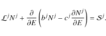
The operator
The coefficients b and c in Eq. (1) are respectively first and second order gains/losses in energy, with
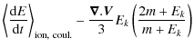
In Eq. (3), the ionisation and Coulomb energy losses are taken from Mannheim & Schlickeiser (1994) and Strong & Moskalenko (1998). The divergence of the Galactic wind
where
The source term ![]() is a combination of i) primary sources
is a combination of i) primary sources ![]() of CRs (e.g., supernovae); ii) secondary fragmentation-induced
sources
of CRs (e.g., supernovae); ii) secondary fragmentation-induced
sources ![]() ;
and iii) secondary decay-induced sources
;
and iii) secondary decay-induced sources ![]() .
In particular, the secondary contributions link one
species to all heavier nuclei, coupling together the n equations.
However, the matrix is triangular and one possible approach is
to solve the equation starting from the heavier nucleus (which is
always assumed to be a primary).
.
In particular, the secondary contributions link one
species to all heavier nuclei, coupling together the n equations.
However, the matrix is triangular and one possible approach is
to solve the equation starting from the heavier nucleus (which is
always assumed to be a primary).
2.2 Geometry of the Galaxy and simplifying assumptions
The Galaxy is modelled to be a thin disc of half-thickness h,
which contains the gas and the
sources of CRs. This disc is embedded in a cylindrical diffusive halo
of half-thickness L, where the gas density
is assumed to be 0. CRs diffuse into both the disc and the
halo independently of their position. A constant wind ![]() perpendicular
to the Galactic plane is also considered.
This is summarised in Fig. 1
(see next section for the definition of
perpendicular
to the Galactic plane is also considered.
This is summarised in Fig. 1
(see next section for the definition of ![]() ).
).
| Figure 1:
Sketch of the model: sources and interactions (including energy losses
and gains) are restricted to the thin disc |
|
| Open with DEXTER | |
We use the ![]() approximation introduced in Jones
(1979), Ptuskin
& Soutoul (1990), and Webber et al. (1992).
Considering the radial extension R of the
Galaxy to be either infinite or finite leads to the 1D version
or 2D version of the model, respectively. The corresponding
sets of equations (and their solutions) obtained after these
simplifications are presented in Appendix A. These
assumptions allow for semi-analytical solutions of the problem,
as the interactions (destruction, spallations, energy gain and
losses) are restricted to the thin disc. The gain is in the computing
time, which is a prerequisite for the use of the
MCMC technique, where several tens of thousands of models are
calculated. These semi-analytical models reproduce all salient features
of full numerical approaches (e.g., Strong
& Moskalenko 1998), and they are useful for
systematically studying the dependence on key parameters,
or some systematics of the parameter determination (Maurin et al. 2010).
approximation introduced in Jones
(1979), Ptuskin
& Soutoul (1990), and Webber et al. (1992).
Considering the radial extension R of the
Galaxy to be either infinite or finite leads to the 1D version
or 2D version of the model, respectively. The corresponding
sets of equations (and their solutions) obtained after these
simplifications are presented in Appendix A. These
assumptions allow for semi-analytical solutions of the problem,
as the interactions (destruction, spallations, energy gain and
losses) are restricted to the thin disc. The gain is in the computing
time, which is a prerequisite for the use of the
MCMC technique, where several tens of thousands of models are
calculated. These semi-analytical models reproduce all salient features
of full numerical approaches (e.g., Strong
& Moskalenko 1998), and they are useful for
systematically studying the dependence on key parameters,
or some systematics of the parameter determination (Maurin et al. 2010).
We note that most of the results of the paper are based on the
1D geometry (solutions only depend on z),
which is less time-consuming than the 2D one in terms of computing time![]() . The parameter degeneracy
is also more easily extracted and understood in this case (Maurin
et al. 2006; Jones et al. 2001).
Nevertheless, the results for the 2D geometry are
also reported, as it has been used in a series of studies inspecting
stable nuclei (Maurin et al. 2001,2002),
. The parameter degeneracy
is also more easily extracted and understood in this case (Maurin
et al. 2006; Jones et al. 2001).
Nevertheless, the results for the 2D geometry are
also reported, as it has been used in a series of studies inspecting
stable nuclei (Maurin et al. 2001,2002),
![]() -radioactive
nuclei (Donato
et al. 2002), standard anti-nuclei (Donato
et al. 2009,2001,2008)
and positrons (Delahaye
et al. 2009). It has also been used to set
constraints on dark matter annihilations in anti-nuclei (Donato et al. 2004),
and positrons (Delahaye
et al. 2008). The reader is referred to these
papers, and especially Maurin
et al. (2001) for more details and references about
the 2D case.
-radioactive
nuclei (Donato
et al. 2002), standard anti-nuclei (Donato
et al. 2009,2001,2008)
and positrons (Delahaye
et al. 2009). It has also been used to set
constraints on dark matter annihilations in anti-nuclei (Donato et al. 2004),
and positrons (Delahaye
et al. 2008). The reader is referred to these
papers, and especially Maurin
et al. (2001) for more details and references about
the 2D case.
2.3 Radioactive species and the local bubble
Our model does not take into account all the observed irregularities of the gas distribution, such as holes, chimneys, shell-like structures, and disc flaring. The main reason is that as far as stable nuclei are concerned, only the average grammage crossed is relevant when predicting their flux (which motivates LBM). As such, the thin-disc approximation is a good trade-off between having a realistic description of the structure of the Galaxy and simplicity.
However, the local distribution of gas affects the flux
calculation of radioactive species
(Ptuskin
& Soutoul 1998; Donato et al. 2002;
Ptuskin
et al. 1997).
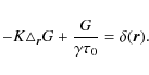
We consider a radioactive nucleus that diffuses in an unbound volume
and decays with a rate
![]() .
In spherical coordinates, appropriate to describe this
situation, the diffusion equation reads
.
In spherical coordinates, appropriate to describe this
situation, the diffusion equation reads
|
(6) |
The solution for the propagator G (the flux is measured at
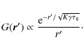
|
(7) |
Secondary radioactive species, such as 10Be, originate from the spallations of the CR protons (and He) with the ISM. We model the source term to be a thin gaseous disc, except in a circular region of radius
| (8) |
where
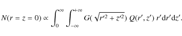
|
(9) |
The ratio of the flux calculated for a cavity/hole
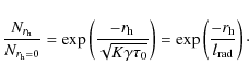
The quantity
In this paper, we model the local bubble to be this simple
hole in the gaseous disc, as shown
in Fig. 1.
The exponential decrease in the flux of this modified DM,
as given by Eq. (10),
is directly plugged into the solutions for the
standard DM (
![]() ). In principle,
i) the hole has also an impact on stable species as it
decreases the amount of matter available for spallations; and
ii) in the 2D geometry, a hole at
). In principle,
i) the hole has also an impact on stable species as it
decreases the amount of matter available for spallations; and
ii) in the 2D geometry, a hole at ![]() kpc
breaks down the cylindrical geometry. However, in practice, Donato et al. (2002)
found that the first effect is minor, and that the hole can always be
taken to be the origin of the Galaxy (the impact of the R boundary
being negligible for radioactive species).
kpc
breaks down the cylindrical geometry. However, in practice, Donato et al. (2002)
found that the first effect is minor, and that the hole can always be
taken to be the origin of the Galaxy (the impact of the R boundary
being negligible for radioactive species).
Other subleties exist, which were not considered in Donato et al. (2002).
Indeed, the damping in the solar neighbourhood -
combined with the production of the radioactive species matching the
data at low energy - means that at intermediate
GeV/n energies, the flux of this radioactive species
is higher in the modified model (with ![]() )
than in the standard one (with
)
than in the standard one (with ![]() ).
It also means that everywhere else in the Galactic disc,
at all energies, the radioactive fluxes are higher in
the modified model (with damping). There are two consequences:
i) all spallative products from these radioactive nuclei
originate in an effective diffusion region in the disc (Taillet & Maurin 2003),
the size of which may be much larger than the size of the
underdense bubble. In this case, these products ought to be
calculated from the undamped fluxes; ii) the decay products of
these radioactive nuclei (e.g., 10B,
which originates from the
).
It also means that everywhere else in the Galactic disc,
at all energies, the radioactive fluxes are higher in
the modified model (with damping). There are two consequences:
i) all spallative products from these radioactive nuclei
originate in an effective diffusion region in the disc (Taillet & Maurin 2003),
the size of which may be much larger than the size of the
underdense bubble. In this case, these products ought to be
calculated from the undamped fluxes; ii) the decay products of
these radioactive nuclei (e.g., 10B,
which originates from the ![]() -decay of 10Be)
are stable species that originate in an effective diffusion sphere
(decay can occur not only in the disc, but in the halo). Both these
effects must be considered because their contributions potentially
affect the calculation, e.g., of the B/C and Be/B ratios
(by means of the B flux), which are used to fit the
models. We confirm that taking spallative products from the damped or
undamped radioactive fluxes left these ratios unchanged. On the other
hand, for the decay products, the effect is of the order of
-decay of 10Be)
are stable species that originate in an effective diffusion sphere
(decay can occur not only in the disc, but in the halo). Both these
effects must be considered because their contributions potentially
affect the calculation, e.g., of the B/C and Be/B ratios
(by means of the B flux), which are used to fit the
models. We confirm that taking spallative products from the damped or
undamped radioactive fluxes left these ratios unchanged. On the other
hand, for the decay products, the effect is of the order of ![]() ,
which is in general enough to change the values of the best-fit
parameters. However, the average flux (over the
effective diffusion zone) from which the decay products originate lies
between the damped and undamped values: the lower the
effective diffusive sphere, the closer the flux is to the
damped one. In particular, at low energy,
when convection is allowed, the diffusion zone can be small (Taillet & Maurin 2003).
,
which is in general enough to change the values of the best-fit
parameters. However, the average flux (over the
effective diffusion zone) from which the decay products originate lies
between the damped and undamped values: the lower the
effective diffusive sphere, the closer the flux is to the
damped one. In particular, at low energy,
when convection is allowed, the diffusion zone can be small (Taillet & Maurin 2003).
To keep the approach simple, we use here the damped flux of
radioactive species for all spallative and decay products
(as was implicitly assumed in Donato et al. 2002).
This approach is expected to provide the maximal possible size
for ![]() (if a non-null value is preferred by the fit).
(if a non-null value is preferred by the fit).
2.4 Input ingredients and free parameters of the study
2.4.1 Gas density
The gas density scale height strongly varies with r
depending on the form considered - neutral, molecular,
or ionised (see, e.g., Ferrière 2001). We use
the surface density measured in the solar neighbourhood as a good
estimate of the average gas in the Galactic disc. We set ![]() cm-3,
which corresponds to a surface density
cm-3,
which corresponds to a surface density ![]()
![]() 1020 cm-2 (Ferrière 2001). The
number fraction of H and He is taken to be 90%
and 10%, respectively. The ionised-hydrogen space-averaged
density may be identified with the free-electron space-averaged
density, which is the sum of the contributions of H
1020 cm-2 (Ferrière 2001). The
number fraction of H and He is taken to be 90%
and 10%, respectively. The ionised-hydrogen space-averaged
density may be identified with the free-electron space-averaged
density, which is the sum of the contributions of H![]() regions
and the diffuse component (Gómez et al. 2001;
Ferrière
2001). The intensity of the latter is well measured
0.018
regions
and the diffuse component (Gómez et al. 2001;
Ferrière
2001). The intensity of the latter is well measured
0.018 ![]() 0.002 cm-3 (Berkhuijsen et al. 2006;
Berkhuijsen
& Müller 2008), whereas the former depends strongly
on the Galactocentric radius r (Anderson & Bania 2009).
For the total electron density, we choose to set
0.002 cm-3 (Berkhuijsen et al. 2006;
Berkhuijsen
& Müller 2008), whereas the former depends strongly
on the Galactocentric radius r (Anderson & Bania 2009).
For the total electron density, we choose to set ![]() and
and ![]() (Nordgren et al.
1992).
(Nordgren et al.
1992).
The disc half-height is set to be h=100 pc.
It is not a physical parameter per se in the ![]() approximation,
although it is related to the phenomena occurring in the thin disc.
Physical parameters are related to the surface density, which is easily
rescaled from that calculated setting h=100 pc
(should we use a different h value). In
the 2D geometry, the boundary is set to be R=20 kpc
and the sun is located at
approximation,
although it is related to the phenomena occurring in the thin disc.
Physical parameters are related to the surface density, which is easily
rescaled from that calculated setting h=100 pc
(should we use a different h value). In
the 2D geometry, the boundary is set to be R=20 kpc
and the sun is located at ![]() kpc.
kpc.
2.4.2 Fragmentation cross-sections
In Paper I, the sets of fragmentation cross-sections were taken from the semi-empirical formulation of Webber et al. (1990) updated in Webber et al. (1998) (see also Maurin et al. 2001, and references therein). In this paper, they are replaced by the 2003 version, as given in Webber et al. (2003). Spallations on He are calculated with the parameterisation of Ferrando et al. (1988).
2.4.3 Source spectrum
We assume that a universal source spectrum for all nuclei
exists, and that it has a simple power-law description. As in
Paper I, we assume that ![]() .
The parameter
.
The parameter ![]() is the spectral index of the sources and
is the spectral index of the sources and ![]() encodes the behaviour of the spectrum at low energy. The normalisations
of the spectra are given by the source abundances qj,
which are renormalised during the propagation step to match the data at
a specified kinetic energy per nucleon (usually
encodes the behaviour of the spectrum at low energy. The normalisations
of the spectra are given by the source abundances qj,
which are renormalised during the propagation step to match the data at
a specified kinetic energy per nucleon (usually ![]() GeV/n). The
correlations between the source and the transport parameters and their
impact on the transport parameter determination were discussed in
Paper I. In this study, we set
GeV/n). The
correlations between the source and the transport parameters and their
impact on the transport parameter determination were discussed in
Paper I. In this study, we set ![]() and
and ![]() (Ave et al. 2008).
Constraints on the source spectra from the study of the measured
primary fluxes are left to a subsequent paper (Donato et al.,
in prep.).
(Ave et al. 2008).
Constraints on the source spectra from the study of the measured
primary fluxes are left to a subsequent paper (Donato et al.,
in prep.).
2.4.4 Free parameters
We have two geometrical free parameters
- L, the halo size of the Galaxy (kpc);
 ,
the size of the local bubble (kpc), which is most of the time set to
be 0 (to compare with models in the literature that
do not consider any local underdensity);
,
the size of the local bubble (kpc), which is most of the time set to
be 0 (to compare with models in the literature that
do not consider any local underdensity);
- K0, the normalisation of the diffusion coefficient (in unit of kpc2 Myr-1);
 ,
the slope of the diffusion coefficient;
,
the slope of the diffusion coefficient;
 ,
the constant convective wind perpendicular to the disc (km s-1);
,
the constant convective wind perpendicular to the disc (km s-1);
 ,
the Alfvénic speed (km s-1) regulating
the reacceleration strength (see Eq. (5)).
,
the Alfvénic speed (km s-1) regulating
the reacceleration strength (see Eq. (5)).

3 MCMC
The MCMC method, based on the Bayesian statistics, is used here to estimate the full distribution - the so-called conditional probability-density function (PDF) - given some experimental data (and some prior density for these parameters). We summarise below the salient features of the MCMC technique. A detailed description of the method can be found in Paper I. The issue of the efficiency, which was not raised in Paper I, is discussed in Appendix C.
The Bayesian approach aims to assess the extent to which an
experimental dataset improves our knowledge of a given theoretical
model. Considering a model depending on m parameters
we wish to determine the PDF of the parameters given the data,
where
In general, MCMC methods attempt to studying any target
distribution of a vector of
parameters, here ![]() ,
by generating a sequence of n
points/steps (hereafter a chain)
,
by generating a sequence of n
points/steps (hereafter a chain)
| (14) |
Each
The chain analysis is based on the selection of a subset of points from the chains (to obtain a reliable estimate of the PDF). Some steps at the beginning of the chain are discarded (burn-in length). By construction, each step of the chain is correlated with the previous steps: sets of independent samples are obtained by thinning the chain (over the correlation length). The fraction of independent samples measuring the efficiency of the MCMC is defined to be the fraction of steps remaining after discarding the burn-in steps and thinning the chain. The final results of the MCMC analysis are the target PDF and all marginalised PDFs. They are obtained by merely counting the number of samples within the related region of parameter space.
4 Results for stable species (fixed halo size L)
For stable species, the degeneracy between the normalisation of the
diffusion coefficient K0
and the halo size of the Galaxy L prevents
us from being able to constrain both parameters at the same time. We
choose to set L=4 kpc (we also set ![]() ,
i.e., standard DM). The free transport parameters are
,
i.e., standard DM). The free transport parameters are
![]() .
The classes of models considered are summarised in Table 1. The
reference B/C dataset (denoted dataset F) used for
the analysis is described in Appendix D.1.
.
The classes of models considered are summarised in Table 1. The
reference B/C dataset (denoted dataset F) used for
the analysis is described in Appendix D.1.
Table 1: Classes of models tested in the paper.
![\begin{figure}
\par\includegraphics[width=8.5cm,clip]{aa14010-fig2.eps}
\end{figure}](/articles/aa/full_html/2010/08/aa14010-10/img96.png)
|
Figure 2: From top to bottom: posterior PDFs of models I-III using the B/C constraint (dataset F). The diagonals show the 1D marginalised PDFs of the indicated parameters. Off-diagonal plots show the 2D marginalised posterior PDFs for the parameters in the same column and same line respectively. The colour code corresponds to the regions of increasing probability (from paler to darker shade), and the two contours (smoothed) delimit regions containing, respectively, 68% and 95% (inner and outer contour) of the PDF. |
| Open with DEXTER | |
4.1 PDF for the transport parameters
We begin with the PDFs of the parameters based on the B/C constraint (dataset F) for the various classes of models (I-III). The PDFs are shown in Fig. 2.
The first important feature is that the marginal distributions
of the transport parameters (diagonals) are mostly Gaussian. From the
off-diagonal distributions, we remark that K0
and ![]() are negatively correlated. This originates in the low-energy relation
are negatively correlated. This originates in the low-energy relation ![]() ,
which should remain approximately constant to reproduce the bulk of the
data at GeV/n energy. The diffusion slope
,
which should remain approximately constant to reproduce the bulk of the
data at GeV/n energy. The diffusion slope ![]() is negatively correlated with
is negatively correlated with ![]() ,
which is related to a smaller
,
which is related to a smaller ![]() being obtained if more reacceleration is included. On the other hand,
the positive correlation between
being obtained if more reacceleration is included. On the other hand,
the positive correlation between ![]() and
and ![]() indicates that larger
indicates that larger ![]() are expected for larger wind velocities.
are expected for larger wind velocities.
We show in Table 2 the most
probable values of the transport parameters, as well as their
uncertainties, corresponding to 68% confidence levels (CL) of
the marginalised PDFs. The precision to which the parameters are
obtained is excellent, ranging from a few %
to 10% at most (for the slope of the diffusion
coefficient ![]() in III). This corresponds to statistical uncertainties only.
These uncertainties are of the order of, or smaller
than systematics generated from uncertainties in the input ingredients
(see details in Maurin
et al. 2010).
in III). This corresponds to statistical uncertainties only.
These uncertainties are of the order of, or smaller
than systematics generated from uncertainties in the input ingredients
(see details in Maurin
et al. 2010).
As found in previous studies (e.g., Lionetto et al. 2005),
for pure diffusion/reacceleration models (II), the value of
the diffusion slope ![]() found is low (
found is low (
![]() here). When
convection is included (I and III),
here). When
convection is included (I and III), ![]() is
large (
is
large (
![]() ). This scatter in
). This scatter in ![]() was already observed in Jones
et al. (2001), who also studied different classes of
models. The origin of this scatter is consistent with the
aforementioned correlations in the parameters (see also Maurin et al. 2010).
was already observed in Jones
et al. (2001), who also studied different classes of
models. The origin of this scatter is consistent with the
aforementioned correlations in the parameters (see also Maurin et al. 2010).
The best-fit model parameters (which are not always the most
probable ones) are given in Table 3, along
with the minimal ![]() value
per degree of freedom,
value
per degree of freedom,
![]() d.o.f.
(last column). As found in previous analyses (Maurin
et al. 2001,2002),
the DM with both reacceleration and convection reproduces the
B/C data more accurately than without:
d.o.f.
(last column). As found in previous analyses (Maurin
et al. 2001,2002),
the DM with both reacceleration and convection reproduces the
B/C data more accurately than without: ![]() /d.o.f. = 1.47
for III, 4.90 for II, and 11.6
for I. The B/C ratio associated with these optimal
/d.o.f. = 1.47
for III, 4.90 for II, and 11.6
for I. The B/C ratio associated with these optimal ![]() values
are displayed with the data in Fig. 3. We note that the poor
fit for II (compared to III) is explained by the
departure of the model prediction from high-energy
HEAO-3 data.
values
are displayed with the data in Fig. 3. We note that the poor
fit for II (compared to III) is explained by the
departure of the model prediction from high-energy
HEAO-3 data.
4.2 Sensitivity to the choice of the B/C dataset
For comparison purposes, we now focus on several datasets for the B/C data. Low-energy data points include ACE data, taken during the solar minimum period 1997-1998 (de Nolfo et al. 2006). Close to submission of this paper, another ACE analysis was published (George et al. 2009). The 1997-1998 data points were reanalysed and complemented with data taken during the solar maximum period 2001-2003. The AMS-01 also provided B/C data covering almost the same range as the HEAO-3 data (Tomassetti & AMS-01 Collaboration 2009). Hence, for this section only, we attempt to analyse other B/C datasets that include these components:
- A: HEAO-3 [0.8-40 GeV/n], 14 data points;
- C: HEAO-3 + low energy [0.3-0.5 GeV/n], 22 data points;
- F: HEAO-3 + low + high energy [0.2-2 TeV/n], 31 data points;
- G1: as F, but with new ACE 1997-1998 data, 31 data points;
- G2: as F, but with new ACE 2001-2003 data only, 31 data points;
- G1/2: using both 1997-1998 and 2001-2003 ACE data, 37 data points;
- H: as F, but HEAO-3 replaced by AMS-01 data, 27 data points.
Table 2: Most probable values for B/C data only (L=4 kpc).
Table 3: Best-fit model parameters for B/C data only (L=4 kpc).
![\begin{figure}
\par\includegraphics[width=8.8cm,clip]{aa14010-fig3.eps}
\end{figure}](/articles/aa/full_html/2010/08/aa14010-10/img121.png)
|
Figure 3:
Best-fit ratio for model I (blue-dotted line), II (red-dashed
line), and
model III (black-solid line) using dataset F: IMP7-8,
Voyager1&2, ACE-CRIS, HEAO-3, Spacelab, and CREAM. The curves
are modulated with |
| Open with DEXTER | |
![\begin{figure}
\par\includegraphics[width=8.8cm,clip]{aa14010-fig4.eps}
\end{figure}](/articles/aa/full_html/2010/08/aa14010-10/img122.png)
|
Figure 4:
B/C data used in this section. Shown are the IS data (rescaled
from TOA data using |
| Open with DEXTER | |
The best-fit model parameters for these data are shown in
Table 4.
The low-energy data play an important part in the fitting procedure: ![]() decreases
by 0.1 when going from III-A to III-C, and the diffusion
normalisation is decreased. When the CREAM data at higher
energy are taken into account (III-F), the best-fit diffusion
slope
decreases
by 0.1 when going from III-A to III-C, and the diffusion
normalisation is decreased. When the CREAM data at higher
energy are taken into account (III-F), the best-fit diffusion
slope ![]() again becomes slightly lower (from 0.89 to 0.86), but
CREAM data uncertainty is still too important to be
conclusive. The impact of the low-energy ACE reanalysed data points is
seen when comparing
III-F with III-G1: the scatter between the derived best-fit
parameters is already of the order
of the statistical uncertainty (see Table 2). The data
taken either during the solar minimum period (G1) or the solar
maximum period (G2) cover a different energy range
(see Fig. 4).
The
again becomes slightly lower (from 0.89 to 0.86), but
CREAM data uncertainty is still too important to be
conclusive. The impact of the low-energy ACE reanalysed data points is
seen when comparing
III-F with III-G1: the scatter between the derived best-fit
parameters is already of the order
of the statistical uncertainty (see Table 2). The data
taken either during the solar minimum period (G1) or the solar
maximum period (G2) cover a different energy range
(see Fig. 4).
The
![]() for G2 is greater, which is not surprising, given the abnormal
trend followed by these data (empty circles in Fig. 4).
Nevertheless, it is reassuring to see that they lead to
consistent values of the transport parameters.
for G2 is greater, which is not surprising, given the abnormal
trend followed by these data (empty circles in Fig. 4).
Nevertheless, it is reassuring to see that they lead to
consistent values of the transport parameters.
Table 4: Best-fit model parameters based on different B/C datasets.
If we now replace the HEAO-3 data with the AMS-01 data,
the impact on the fit is striking: the best-fit
diffusion slope ![]() goes from 0.86 to 0.51. As discussed in Maurin et al. (2010),
HEAO-3 data strongly constrain the slope towards
goes from 0.86 to 0.51. As discussed in Maurin et al. (2010),
HEAO-3 data strongly constrain the slope towards ![]() ,
even if there is a systematic energy bias in the HEAO-3 data
themselves. From the AMS-01 data, we see that there could be a way of
reconciling the presence of a Galactic wind and reasonable values
of
,
even if there is a systematic energy bias in the HEAO-3 data
themselves. From the AMS-01 data, we see that there could be a way of
reconciling the presence of a Galactic wind and reasonable values
of ![]() .
However, the large error bars in AMS-01 data, reflected by the
low
.
However, the large error bars in AMS-01 data, reflected by the
low ![]() /d.o.f. value,
does not allow to draw firm conclusions. Data in the same energy range
from PAMELA would be helpful in that respect. Moreover, high energy
data from subsequent CREAM flights or from the TRACER experiments will
be a crucial test of the diffusion slope:
at TeV energies, diffusion alone is expected to shape
the observed spectra, so that the ambiguity with the effect of
convection or reacceleration is lifted (Castellina & Donato 2005).
/d.o.f. value,
does not allow to draw firm conclusions. Data in the same energy range
from PAMELA would be helpful in that respect. Moreover, high energy
data from subsequent CREAM flights or from the TRACER experiments will
be a crucial test of the diffusion slope:
at TeV energies, diffusion alone is expected to shape
the observed spectra, so that the ambiguity with the effect of
convection or reacceleration is lifted (Castellina & Donato 2005).
4.3 Comparison of trends for the DM and for the LBM
For completeness, we briefly comment on the similarities and differences between the results found here and in Paper I. To follow the organisation of the previous sections, the comparison with the LBM is discussed for different classes of models (I-III), and then for different datasets (A-C). We note that the best-fit values presented below differ slightly for those given in Paper I, as an updated set of production cross-section is used.
We recall that in the LBM (see Paper I), the free
parameters are the normalisation of the escape length ![]() ,
,
![]() ,
a cut-off rigidity R0,
and a pseudo-Alfvénic
speed
,
a cut-off rigidity R0,
and a pseudo-Alfvénic
speed
![]() .
The latter is linked to a true speed by means of
.
The latter is linked to a true speed by means of ![]()
![]() (hL)1/2,
i.e.,
(hL)1/2,
i.e., ![]() for h=0.1 kpc and L=4 kpc.
The diffusion coefficient at 1 GV is related to the
escape length by means of
for h=0.1 kpc and L=4 kpc.
The diffusion coefficient at 1 GV is related to the
escape length by means of ![]()
![]()
![]() ,
where we use
,
where we use ![]()
![]() 10-3 g cm-2,
leading to K0 (kpc2 Myr
10-3 g cm-2,
leading to K0 (kpc2 Myr
![]() g cm-2).
The LBM parameters gathered in Table 5 are obtained
from the above conversions, to ease the comparison with the
DM results.
g cm-2).
The LBM parameters gathered in Table 5 are obtained
from the above conversions, to ease the comparison with the
DM results.
Table 5: Best-fit parameters on B/C data for the LBM.
For the different classes of models (I-III), a comparison of
Table 3
with the first three rows of Table 5 indicates
that the same trend is found. For instance, model I
(without reacceleration) has a larger ![]() than those with, and model II (without
convection/rigidity-cutoff) has a smaller
than those with, and model II (without
convection/rigidity-cutoff) has a smaller ![]() than those with. The slope for model III (with both convection
and reacceleration) is in-between. This effect is more marked for the
DM than for the LBM. We note that model II (with
reacceleration but without convection) is almost consistent with a
Kolmogorov spectrum of turbulence, but is inconsistent with
the data. Concerning the different datasets (A, C,
and F), again, the same trend as for the LBM is found
(compare Table 4
and the last three rows of Table 5).
than those with. The slope for model III (with both convection
and reacceleration) is in-between. This effect is more marked for the
DM than for the LBM. We note that model II (with
reacceleration but without convection) is almost consistent with a
Kolmogorov spectrum of turbulence, but is inconsistent with
the data. Concerning the different datasets (A, C,
and F), again, the same trend as for the LBM is found
(compare Table 4
and the last three rows of Table 5).
The most striking difference between the two models (LBM and
DM) concerns their ![]() values.
This difference can be explained in terms of non-equivalent
parameterisation of the low-energy transport coefficient (see Maurin et al. 2010,
for more details). Apart from this, both the value of the Alfvénic
speed and the normalisation of the diffusion coefficient K0
in the two cases are fairly consistent when similar values of
values.
This difference can be explained in terms of non-equivalent
parameterisation of the low-energy transport coefficient (see Maurin et al. 2010,
for more details). Apart from this, both the value of the Alfvénic
speed and the normalisation of the diffusion coefficient K0
in the two cases are fairly consistent when similar values of ![]() are considered.
are considered.
4.4 Dependence of the parameters with L
All the previous conclusions were derived for L=4 kpc, but hold for any other halo size. The evolution of the transport parameters with L is shown in Fig. 5 (the best-fit values are consistent with those found in Maurin et al. 2002). In the three upper figures, we have superimposed the observed dependence a parametric formula.
For K0 (top panel),
the formula can be understood if we consider the grammage of
the DM. In the purely diffusive regime, we have ![]() .
This means that when we vary L, to keep the
same grammage in the equivalent LBM, we need to
vary K0 accordingly. We find
that K0=1.08
.
This means that when we vary L, to keep the
same grammage in the equivalent LBM, we need to
vary K0 accordingly. We find
that K0=1.08 ![]()
![]() kpc2 Myr-1
instead of
kpc2 Myr-1
instead of ![]() .
The origin of the residual L1.06
dependence is unclear. It may come from the energy loss and
gain terms.
.
The origin of the residual L1.06
dependence is unclear. It may come from the energy loss and
gain terms.
![\begin{figure}
\par\includegraphics[width=8.8cm,clip]{aa14010-fig5.eps}
\end{figure}](/articles/aa/full_html/2010/08/aa14010-10/img135.png)
|
Figure 5:
Best-fit parameters (III-F) as a function of the halo size of the
Galaxy (blue circles). From top to bottom: K0, |
| Open with DEXTER | |
For the reacceleration, the interpretation is also simple. From
Eq. (5),
![]() should
scale as
should
scale as ![]() ,
so that
,
so that ![]() .
We find
.
We find ![]() km s-1.
This is exactly
km s-1.
This is exactly ![]() ,
with the dependence
,
with the dependence
![]() as above. The quantities
as above. The quantities ![]() and
and ![]() are roughly constant with L. The
are roughly constant with L. The ![]() surface
is rather flat, although a minimum is observed around
surface
is rather flat, although a minimum is observed around ![]() kpc
(the presence of a minimum may be related to the presence of
the decayed 10Be into 10B
in the B/C ratio). This flatness is a consequence of the
degeneracy of K0/L
when only stable species are considered. Consequently, an MCMC
with L as an additional free parameter does
not converge to the stationary distribution. A sampling of the
Galactic halo size is possible if radioactive nuclei are considered to
lift the above degeneracy (see Sect. 5).
kpc
(the presence of a minimum may be related to the presence of
the decayed 10Be into 10B
in the B/C ratio). This flatness is a consequence of the
degeneracy of K0/L
when only stable species are considered. Consequently, an MCMC
with L as an additional free parameter does
not converge to the stationary distribution. A sampling of the
Galactic halo size is possible if radioactive nuclei are considered to
lift the above degeneracy (see Sect. 5).
4.5 Summary of stable species and generalisation to the 2D geometry
The transport parameters for both LBM (Paper I) and
1D DM, when fitted to existing B/C data, are
consistent with both convection and reacceleration. The correlations
between the various transport parameters, as calculated from the
MCMC technique, are consistent with what is expected from the
relationships between DMs and the LBM (e.g., Maurin et al. 2006).
From the B/C analysis point of view, it implies that
even if we areunable to reach conclusions about the value
of ![]() (see Maurin
et al. 2010), once this value is known, all other
transport parameters are well constrained.
(see Maurin
et al. 2010), once this value is known, all other
transport parameters are well constrained.
The conclusions obtained for the 1D DM naturally hold for the
2D DM. We recall that the main difference between the 1D and
2D geometry is that i) the spatial distribution of
sources, which
was constant in 1D, is now q(r);
and ii) the Galaxy has a side-boundary at a radius taken to
be R=20 kpc. As a check,
we first used the 2D solution (presented in Appendix A.2) with
R=20 kpc, but set q(r)
to be constant. The best-fit parameters were in agreement with those
obtained from the 1D solution. We present in Table 6 the best-fit
parameters
for models II and III for L=4 kpc
in the 2D solution where q(r)
follows the SN remnant distribution of Case & Bhattacharya
(1998). The values for the 1D solution are also
reported
for the sake of comparison. The main difference is in the value
of K0, which varies
by ![]() and also affects
and also affects ![]() (by means of the ratio
(by means of the ratio ![]() ,
which
is left unaffected). This is consistent with the variations found by Maurin et al. (2002).
,
which
is left unaffected). This is consistent with the variations found by Maurin et al. (2002).
Table 6: Best-fit model parameters on B/C data: 1D versus 2D DM (L=4 kpc).
![\begin{figure}
\par\includegraphics[width=14cm,clip]{aa14010-fig6.eps}
\end{figure}](/articles/aa/full_html/2010/08/aa14010-10/img143.png)
|
Figure 6:
Model II (diffusion/reacceleration): marginalised posterior PDF of the
diffusive halo size L (right panels
of the first and second row) and the local bubble radius |
| Open with DEXTER | |
![\begin{figure}
\par\includegraphics[width=15cm,clip]{aa14010-fig7.eps}
\end{figure}](/articles/aa/full_html/2010/08/aa14010-10/img144.png)
|
Figure 7:
Model III (diffusion/convection/reacceleration): same as in
Fig. 6.
The transport parameters are now |
| Open with DEXTER | |
5 Results for radioactive species (free halo size L)
We now attempt to lift the degeneracy between the halo size and the
normalisation of the diffusion coefficient, using radioactive nuclei.
The questions that we wish to address are the following:
i) with existing data, how large are the uncertainties
in L for a given model?
ii) Do radioactive nuclei provide different answers
for models with different ![]() ? iii) Is the mean
value (and uncertainty) for L
obtained from a given isotopic/elemental ratio consistent with or
stronger constrained than that obtained from another measured
isotopic/elemental ratio? iv) How does the presence of a local
underdense bubble (modelled as a hole of radius
? iii) Is the mean
value (and uncertainty) for L
obtained from a given isotopic/elemental ratio consistent with or
stronger constrained than that obtained from another measured
isotopic/elemental ratio? iv) How does the presence of a local
underdense bubble (modelled as a hole of radius ![]() ,
see Sect. 2.3)
affect the conclusions?
,
see Sect. 2.3)
affect the conclusions?
Until now, almost all studies have focused on the isotopic ratios of 10Be/9Be, 26Al/27Al, 36Cl/Cl, and 54Mn/Mn. An alternative, discussed in Webber & Soutoul (1998), is to consider the Be/B, Al/Mg, Cl/Ar, and Mn/Fe ratios. The advantage of considering these elemental ratios is that they are easier to measure than isotopic ratios, and thus provide a wider energy range to which we can fit the data. Taking ratios such as Be/B maximises the effect of radioactive decay, since the numerator represents the decaying nucleus and the denominator the decayed nucleus. However, the radioactive contribution is only a fraction of the elemental flux, and HEAO-3 data were found to be less constraining that the isotopic ratios in Webber & Soutoul (1998).
Below, we consider and compare the constraints from both the
isotopic ratios and the elemental ratios. The data used are described
in Appendix D.2.
We discard 54Mn because it suffers more
uncertainties than the others in the calculation (and also
experimentally) due to the electron capture decay channel. The free
parameters for which we seek the PDF are the four transport
parameters
![]() ,
plus one
,
plus one ![]() or two geometrical parameters
or two geometrical parameters
![]() ,
depending on the configuration considered. The main results of this
section are thus in identifying the PDF of L
for the standard DM, and the PDFs of both L
and
,
depending on the configuration considered. The main results of this
section are thus in identifying the PDF of L
for the standard DM, and the PDFs of both L
and ![]() for the modified DM.
for the modified DM.
5.1 PDFs of L and rh using isotopic measurements
We start with a simultaneous fit to B/C and 10Be/9Be, for both model III (diffusion/convection/reacceleration), and model II (diffusion/reacceleration), the latter being frequently used in the literature.
5.1.1 Simultaneous fit to B/C and 10Be/9Be
The marginalised posterior PDFs of L and ![]() and the correlations between these new free parameters and the
propagation parameters of models II and III are given
in the Figs. 6
and 7,
respectively. The most probable values of the parameters are gathered
in Table 7.
and the correlations between these new free parameters and the
propagation parameters of models II and III are given
in the Figs. 6
and 7,
respectively. The most probable values of the parameters are gathered
in Table 7.
Table 7:
Most probable values for models II and III for the
free parameters of the local bubble radius ![]() and/or the Galactic halo size L
(constrained by B/C and 10Be/9Be data).
and/or the Galactic halo size L
(constrained by B/C and 10Be/9Be data).
For all configurations, the diffusion slope ![]() and the Galactic wind
and the Galactic wind ![]() are unaffected by the addition of the free parameters L
and
are unaffected by the addition of the free parameters L
and ![]() .
The B/C fit is degenerate in K0/L
and
.
The B/C fit is degenerate in K0/L
and
![]() ,
so that the values of K0
and
,
so that the values of K0
and ![]() vary as L varies. For model III,
their evolution follows the relations given in Fig. 5. This
implies that there is a positive correlation between K0
and
vary as L varies. For model III,
their evolution follows the relations given in Fig. 5. This
implies that there is a positive correlation between K0
and ![]() ,
and K0 and L,
as seen from Figs. 6
and 7.
The uncertainty in the diffusive halo size L
is smaller for II than for III. This is a consequence
of the inclusion of the constant wind, which decreases the resolution
on K0
from 2% (Model II) to 10%
(Model III) - see e.g., Tables 2
or 7
- hence broadening the distribution of L.
,
and K0 and L,
as seen from Figs. 6
and 7.
The uncertainty in the diffusive halo size L
is smaller for II than for III. This is a consequence
of the inclusion of the constant wind, which decreases the resolution
on K0
from 2% (Model II) to 10%
(Model III) - see e.g., Tables 2
or 7
- hence broadening the distribution of L.
Below, the results for the standard DM - for which ![]() is set to be 0 - and those for the modified DM - for which
is set to be 0 - and those for the modified DM - for which ![]() is left as an additional free parameter - are discussed separately.
This allows us to emphasise the impact of
is left as an additional free parameter - are discussed separately.
This allows us to emphasise the impact of ![]() on the other parameters, which
is different for models II and III.
on the other parameters, which
is different for models II and III.
Standard
DM (
 ):
):
the parameter L is constrained to be
between 4.6 and Modified
DM (
 ):
):
the presence of a local bubble results in an exponential attenuation of
the local radioactive flux, see Sect. 2.3 and
Eq. (10).
We thus expect to have a different best-fit parameter for L
in that case. The resulting posterior PDFs of L
and As expected, the local bubble radius ![]() is negatively correlated with the Galactic halo size L.
The effect is more striking for model III, where the favoured
range for L extends from 1
to 50 kpc. The most probable value is
is negatively correlated with the Galactic halo size L.
The effect is more striking for model III, where the favoured
range for L extends from 1
to 50 kpc. The most probable value is ![]() kpc
for a local bubble radius
kpc
for a local bubble radius ![]() .
The
.
The ![]() /d.o.f.
of this configuration is 1.28, instead of 1.41 for
the standard DM. The improvement to the fit is statistically
significant according to the Fisher criterion.
/d.o.f.
of this configuration is 1.28, instead of 1.41 for
the standard DM. The improvement to the fit is statistically
significant according to the Fisher criterion.
The situation for model II is different. The halo
size L is already small for the standard
configuration ![]() .
Adding the local bubble radius
.
Adding the local bubble radius ![]() to the fit decreases the most probable value of L
only slightly to
to the fit decreases the most probable value of L
only slightly to ![]() and the measured value of
and the measured value of ![]() is compatible with 0 pc. In addition, the
is compatible with 0 pc. In addition, the ![]() /d.o.f.
is 3.69 and hence poorer than for the configuration without
the local bubble feature. In this model
(diffusion/reacceleration, no convection), a local
underdensity is not supported.
/d.o.f.
is 3.69 and hence poorer than for the configuration without
the local bubble feature. In this model
(diffusion/reacceleration, no convection), a local
underdensity is not supported.
5.1.2 Results and comparison with fits to 26Al/27Al and 36Cl/Cl
We repeat the analysis for the remaining isotopic ratios. The resulting
marginalised posterior PDFs of the Galactic halo size L
and the local underdensity ![]() are given in Figs. 8
and 9
for models II and III, respectively. The correlation
plots with the transport parameters are similar to those of
Figs. 6
and 7
and are not repeated.
are given in Figs. 8
and 9
for models II and III, respectively. The correlation
plots with the transport parameters are similar to those of
Figs. 6
and 7
and are not repeated.
![\begin{figure}
\par\includegraphics[width=8.8cm,clip]{aa14010-fig8.eps}
\end{figure}](/articles/aa/full_html/2010/08/aa14010-10/img180.png)
|
Figure 8:
Model II: marginalised posterior PDFs of the Galactic geometry
parameters for the standard DM (
|
| Open with DEXTER | |
![\begin{figure}
\par\includegraphics[width=8.8cm,clip]{aa14010-fig9.eps}
\end{figure}](/articles/aa/full_html/2010/08/aa14010-10/img181.png)
|
Figure 9: Same as in Fig. 8, but for model III. |
| Open with DEXTER | |
Standard
DM (
):
as for the 10Be/9Be ratio
(red-dotted line), L is well constrained
in model II at small values for the 26Al/27Al
(green-long dashed-dotted line), and 36Cl/Cl
(blue dashed-dotted line) ratios, covering slightly different but
consistent ranges from 4 to 14 kpc. The width of the
estimated PDFs increases when moving from the 10Be/9Be ratio
to the 36Cl/Cl ratio, due to
the decreasing accuracy of the data. In the same way, the
adjustment to the data becomes poorer, as expressed by the increase
in The best-fit model is model III, where the overall
covered halo size range extends from 20
to 140 kpc. The most probable value found
for L with 68% confidence level
(CL) errors is
![]() .
.
Modified
DM (
):
the resulting marginalised posterior PDFs of L
are shown in Figs. 8
and 9
(lower left) for models II and III, respectively.
Again, the extracted PDFs for all radioactive ratios are
completely compatible for both models. As described above, the
decrease in L is more pronounced for
model III than for model II. This decrease can be
observed for all radioactive ratios, independently of the model chosen.
The resulting marginalised posterior PDFs of ![]() are given in Figs. 8
and 9
(lower right) for models II and III, respectively.
The addition of an underdensity in the local interstellar medium is
preferred by the data in the best-fit model III,
but it is disfavoured in model II. The most probable
values for
are given in Figs. 8
and 9
(lower right) for models II and III, respectively.
The addition of an underdensity in the local interstellar medium is
preferred by the data in the best-fit model III,
but it is disfavoured in model II. The most probable
values for ![]() range from 90 pc for the 36Cl/Cl ratio
to 140 pc for the the 26Al/27Al ratio,
and the overall fit points to a most probable radius of
130+10-20 pc.
range from 90 pc for the 36Cl/Cl ratio
to 140 pc for the the 26Al/27Al ratio,
and the overall fit points to a most probable radius of
130+10-20 pc.
These results confirm and extend the slightly different
analysis of Donato
et al. (2002), who found that for
model III, the best-fit values for ![]() was
was ![]() pc
(see also Appendix B).
pc
(see also Appendix B).
5.1.3 Envelopes of 68% CL
Confidence contours (for any combination of the CR fluxes)
corresponding to given confidence levels (CL) in the ![]() distribution
can be drawn, as detailed in Appendix A and
Sect. 5.1.4 of Paper I. From the
MCMC calculation based on the B/C + 10Be/9Be +
26Al/27Al + 36Cl/Cl
constraint, we select all sets of parameters for which the
distribution
can be drawn, as detailed in Appendix A and
Sect. 5.1.4 of Paper I. From the
MCMC calculation based on the B/C + 10Be/9Be +
26Al/27Al + 36Cl/Cl
constraint, we select all sets of parameters for which the ![]() meets
the 68% confidence level criterion. For each set of
these parameters, we calculate the B/C and the three isotopic ratios.
We store for each energy the minimum and maximum value of the ratio.
The
corresponding contours (along with the best-fit ratio) for
models II (standard DM, red) and III (standard and
modified DM, blue) are drawn in Fig. 10.
To ease the comparison with the data, all results correspond
to IS quantities (the approximation made in the
demodulation procedure, see Paper I, is negligible
with respect to the experimental error bars).
meets
the 68% confidence level criterion. For each set of
these parameters, we calculate the B/C and the three isotopic ratios.
We store for each energy the minimum and maximum value of the ratio.
The
corresponding contours (along with the best-fit ratio) for
models II (standard DM, red) and III (standard and
modified DM, blue) are drawn in Fig. 10.
To ease the comparison with the data, all results correspond
to IS quantities (the approximation made in the
demodulation procedure, see Paper I, is negligible
with respect to the experimental error bars).
![\begin{figure}
\par\includegraphics[width=17cm,clip]{aa14010-fig10.eps}
\end{figure}](/articles/aa/full_html/2010/08/aa14010-10/img185.png)
|
Figure 10:
Shown are the envelopes of 68% CL (shaded areas) and best-fit
(thick lines) ratios for the standard DM II (
|
| Open with DEXTER | |
We see that the present data already constrain very well the various
ratios for the standard DM. The difference between the results
of models II and III are more pronounced at high
energy (effect of ![]() ),
as seen from the B/C ratio beyond 10 GeV/n.
All contours are pinched around 10 GeV/n, which is a
consequence of the energy chosen to renormalise the flux to the data in
the propagation code. In principle, the source
abundance of each species may be set as an additional free parameter in
the fit (Paper I), but at the cost of the computing time. The
three isotopic ratios (10Be/9Be26,
Al/27Al, and 36Cl/Cl)
provide a fair match to the data for all models, considering the large
scatter and possible inconsistencies between the results quoted by
various experiments. In particular, for 10Be/9Be,
new data are necessary to confirm the high value of the ratio measured
at
),
as seen from the B/C ratio beyond 10 GeV/n.
All contours are pinched around 10 GeV/n, which is a
consequence of the energy chosen to renormalise the flux to the data in
the propagation code. In principle, the source
abundance of each species may be set as an additional free parameter in
the fit (Paper I), but at the cost of the computing time. The
three isotopic ratios (10Be/9Be26,
Al/27Al, and 36Cl/Cl)
provide a fair match to the data for all models, considering the large
scatter and possible inconsistencies between the results quoted by
various experiments. In particular, for 10Be/9Be,
new data are necessary to confirm the high value of the ratio measured
at ![]() GeV/n energy.
GeV/n energy.
The envelope for the modified DM is quite large at high
energy, because the uncertainty in ![]() is responsible for a larger scatter in the other parameters. The two
standard DM contain non-overlapping envelopes beyond
GeV/n energies. This means that to disentangle the models,
having measurements of the above isotopic ratios in the
1-10 GeV/n may be more important than just having more and
higher quality data at low energy.
is responsible for a larger scatter in the other parameters. The two
standard DM contain non-overlapping envelopes beyond
GeV/n energies. This means that to disentangle the models,
having measurements of the above isotopic ratios in the
1-10 GeV/n may be more important than just having more and
higher quality data at low energy.
General
dependence of L with
(for
= 0)
To investigate the difference in the results obtained from
models II and III, we fit B/C and the
three isotopic ratios for different values of ![]() (a similar trend with L is
obtained if
just one isotopic ratio is selected). The analysis relies on the Minuit
minimisation routine to
quickly find the best-fit values, as described in Maurin et al. (2010).
The evolution of the parameters with
(a similar trend with L is
obtained if
just one isotopic ratio is selected). The analysis relies on the Minuit
minimisation routine to
quickly find the best-fit values, as described in Maurin et al. (2010).
The evolution of the parameters with ![]() is shown on the left side of Fig. 11. The
bottom panel shows the evolution of
is shown on the left side of Fig. 11. The
bottom panel shows the evolution of ![]() d.o.f.,
where we recover that the best-fit
d.o.f.,
where we recover that the best-fit ![]() for model II (dashed-blue line) lies around
for model II (dashed-blue line) lies around ![]() ,
whereas that for model III (solid-black line) lies around
,
whereas that for model III (solid-black line) lies around ![]() .
As already underlined, the contribution to the
.
As already underlined, the contribution to the ![]() value
is dominated by the B/C contribution because as discussed in
Appendix C,
the values of transport parameters that reproduce the
B/C ratio are expected to remain within a narrow range. This
explains what is observed in the various panels showing these
combinations. For model II, we emphasise that for
value
is dominated by the B/C contribution because as discussed in
Appendix C,
the values of transport parameters that reproduce the
B/C ratio are expected to remain within a narrow range. This
explains what is observed in the various panels showing these
combinations. For model II, we emphasise that for ![]() ,
the best-fit value for
,
the best-fit value for ![]() is zero (Model II becomes a pure diffusion model).
is zero (Model II becomes a pure diffusion model).
![\begin{figure}
\par\includegraphics[width=16cm,clip]{aa14010-fig11.eps}
\end{figure}](/articles/aa/full_html/2010/08/aa14010-10/img190.png)
|
Figure 11:
Left panel: standard DM model (
|
| Open with DEXTER | |
The most important result, given in the top panel, is for L
as a function of ![]() ,
where any uncertainty in the determination of
,
where any uncertainty in the determination of ![]() translates into an uncertainty in the determination of L.
When a Galactic wind is considered (Model III, black-solid
line), the correlation between L
and
translates into an uncertainty in the determination of L.
When a Galactic wind is considered (Model III, black-solid
line), the correlation between L
and ![]() is stronger than for model II (no wind). There is no
straightforward explanation of this dependence. The flux of the
radioactive isotope can be shown to be
is stronger than for model II (no wind). There is no
straightforward explanation of this dependence. The flux of the
radioactive isotope can be shown to be ![]() (e.g., Maurin
et al. 2006). Since secondary fluxes should match
the data regardless of the value for
(e.g., Maurin
et al. 2006). Since secondary fluxes should match
the data regardless of the value for ![]() ,
this implies that the ratio 10Be/9Be
depends only on
,
this implies that the ratio 10Be/9Be
depends only on ![]() .
At the same time, to ensure that the
secondary-to-primary ratio is constant, we must maintain a
constant L/K.
The difficulty is that the former quantity is a constant at
low rigidity where the isotopic ratio is measured, whereas the latter
quantity should remain as close a possible to the B/C data
over the whole energy range. Hence, all we can say is that the
variation in L with
.
At the same time, to ensure that the
secondary-to-primary ratio is constant, we must maintain a
constant L/K.
The difficulty is that the former quantity is a constant at
low rigidity where the isotopic ratio is measured, whereas the latter
quantity should remain as close a possible to the B/C data
over the whole energy range. Hence, all we can say is that the
variation in L with ![]() is related to the variation in K0/L
with
is related to the variation in K0/L
with ![]() ,
as shown in the second figure (left panel) of Fig. 11.
,
as shown in the second figure (left panel) of Fig. 11.
We note that all the calculations in the paper are based on
the W03 (Webber
et al. 2003)
fragmentation cross-sections. The impact of using the W03 set or the
GAL09 set (provided in the widely used GALPROP package![]() ) on the
determination of the halo size L
is shown as thin-dotted lines (left panel, same figure)
) on the
determination of the halo size L
is shown as thin-dotted lines (left panel, same figure)![]() . Any difference existing
between these two sets of production cross-sections has no impact on
the best-fit value for L: thin-dashed
curves (obtained with GAL09 cross-sections) almost match the
thick-solid curves (obtained with W03 cross-sections). For other
ratios, the effect of the GAL09 cross-sections is always the same,
so it is not discussed further.
. Any difference existing
between these two sets of production cross-sections has no impact on
the best-fit value for L: thin-dashed
curves (obtained with GAL09 cross-sections) almost match the
thick-solid curves (obtained with W03 cross-sections). For other
ratios, the effect of the GAL09 cross-sections is always the same,
so it is not discussed further.
General
dependence of L with
(for )
We repeat the analysis with the underdensity ![]() as an additional free parameter. The dependence of L
and
as an additional free parameter. The dependence of L
and ![]() on the diffusion slope
on the diffusion slope ![]() is shown in the right panel of Fig. 11.
A comparison between the left and the right panel shows
that the combinations of parameters K0/L,
is shown in the right panel of Fig. 11.
A comparison between the left and the right panel shows
that the combinations of parameters K0/L,
![]() ,
and
,
and ![]() are almost unaffected by the presence of a local bubble; the
are almost unaffected by the presence of a local bubble; the ![]() d.o.f. is
also only slightly affected.
d.o.f. is
also only slightly affected.
For ![]()
![]() 0.2,
0.2, ![]() is consistent with 0 for both model II
(diffusion/reacceleration) and model III
(diffusion/convection/reacceleration). For model II, the size
of
is consistent with 0 for both model II
(diffusion/reacceleration) and model III
(diffusion/convection/reacceleration). For model II, the size
of ![]() suddenly jumps to
suddenly jumps to ![]() pc.
But for
pc.
But for ![]() ,
it returns to the pure diffusion regime,
,
it returns to the pure diffusion regime, ![]() decreasing
abruptly (to a non-vanishing value) and L
becoming vanishingly small. In this regime,
the thin-disc approximation is no longer valid and nothing can
be said about it. For model III,
the plateau
decreasing
abruptly (to a non-vanishing value) and L
becoming vanishingly small. In this regime,
the thin-disc approximation is no longer valid and nothing can
be said about it. For model III,
the plateau ![]() pc
is stable for all
pc
is stable for all ![]() .
The underdense
bubble also stabilises the value of the halo size L.
The way of understanding this trend is
as for the standard DM, but now the flux of the radioactive
species reads
.
The underdense
bubble also stabilises the value of the halo size L.
The way of understanding this trend is
as for the standard DM, but now the flux of the radioactive
species reads ![]() .
The weaker dependence of L with
.
The weaker dependence of L with ![]() must be represented by this formula. We underline that for all best-fit
configurations leading to
must be represented by this formula. We underline that for all best-fit
configurations leading to ![]() ,
the improvement is statistically meaningful compared to the
case
,
the improvement is statistically meaningful compared to the
case ![]() .
.
5.2 Isotopic versus elemental measurements
A similar analysis can be carried out using elemental ratios instead of
isotopic ones. As before, the best-fit values of
well-chosen combinations of the transport parameters
![]() are left unchanged when radioactive species are added to the fit (same
values as in Fig. 11).
are left unchanged when radioactive species are added to the fit (same
values as in Fig. 11).
5.2.1
General dependence of L with
For the standard DM (
![]() ), the dependence of the
diffusive halo size L on the diffusion
slope
), the dependence of the
diffusive halo size L on the diffusion
slope ![]() is shown in Fig. 12,
for the three combinations B/C + Be/B,
B/C + Al/Mg, and B/C + Cl/Ar. The
trend is similar to that for isotopic ratios: L increases
with increasing
is shown in Fig. 12,
for the three combinations B/C + Be/B,
B/C + Al/Mg, and B/C + Cl/Ar. The
trend is similar to that for isotopic ratios: L increases
with increasing ![]() .
The main difference is that the increase is sharper for both
models II and III. For the former,
only a small region around
.
The main difference is that the increase is sharper for both
models II and III. For the former,
only a small region around ![]() corresponds to small halo sizes. For the latter,
the halo size increases sharply above
corresponds to small halo sizes. For the latter,
the halo size increases sharply above ![]() .
.
For completeness, similar fits were carried out for the
modified DM (
![]() ). However, adding an
additional degree of freedom only worsens the situation, and the models
converge to arbitrarily small or high values of L
and
). However, adding an
additional degree of freedom only worsens the situation, and the models
converge to arbitrarily small or high values of L
and ![]() .
Finally, if we fit the combined B/C data,
the three isotopic ratios and the three elemental ratios, we
do not obtain more constraints than when fitting B/C and the
three isotopic ratios. This may indicate that the models have
difficulties in fitting all these data together: either the model is
incomplete or the data themselves may show some inconsistencies. This
is more clearly seen from the comparison of the model calculation and
the data for these elemental ratios (see below).
.
Finally, if we fit the combined B/C data,
the three isotopic ratios and the three elemental ratios, we
do not obtain more constraints than when fitting B/C and the
three isotopic ratios. This may indicate that the models have
difficulties in fitting all these data together: either the model is
incomplete or the data themselves may show some inconsistencies. This
is more clearly seen from the comparison of the model calculation and
the data for these elemental ratios (see below).
5.2.2 Envelopes of 68% CL
From the same set of constraint as in Sect. 5.1.3 (i.e., B/C and the isotopic ratios of radioactive species only), we draw the CL for the elemental ratios in Fig. 13.
![\begin{figure}
\par\includegraphics[width=8.5cm,clip]{aa14010-fig12.eps}
\end{figure}](/articles/aa/full_html/2010/08/aa14010-10/img198.png)
|
Figure 12:
Best-fit value of the halo size L as a
function of |
| Open with DEXTER | |
![\begin{figure}
\par\includegraphics[width=8.5cm,clip]{aa14010-fig13.eps}
\vspace*{4mm}
\end{figure}](/articles/aa/full_html/2010/08/aa14010-10/img199.png)
|
Figure 13: Same as in Fig. 10 but for the ratios Be/B, Al/Mg, and Cl/Ar. |
| Open with DEXTER | |
Given their large error bars, the elemental ratios are in overall agreement with the data, except at low energy and especially for the Be/B ratio. The main difference between the Be/B ratio and the two other ratios is that Be and B are pure secondary species, whereas all other elements may contain some primary contribution which can be adjusted to more closely match the data. This also explains why the Be/B ratio reaches an asymptotical value at high energy (related to the respective production cross-sections of Be and B), whereas the two others exhibit more complicated patterns. The low-energy Be/B ratio is related to either the model or the energy biases in the production cross-sections for these elements (which is still possible, e.g. Webber et al. 2003), or to systematics in the data. To solve this issue, better data over the whole energy range are required.
5.3 Summary and generalisation to the 2D geometry
Using radioactive nuclei in the 1D geometry, we found that in
model II (diffusion/reacceleration),
![]() kpc
and
kpc
and ![]() ,
and for the best-fit model III
(diffusion/convection/reacceleration),
,
and for the best-fit model III
(diffusion/convection/reacceleration), ![]() kpc and
kpc and ![]() pc.
The halo size is an increasing function of the diffusion slope
pc.
The halo size is an increasing function of the diffusion slope ![]() ,
but in model III the best-fit value for
,
but in model III the best-fit value for ![]() remains
remains ![]() pc
for any
pc
for any ![]() .
This value agrees with direct observation of the LISM
(see Appendix B).
Measurement of elemental ratios of radioactive species are not yet
precise enough to provide valuable constraints.
.
This value agrees with direct observation of the LISM
(see Appendix B).
Measurement of elemental ratios of radioactive species are not yet
precise enough to provide valuable constraints.
For now, there are too large uncertainties and too many inconsistencies between the data themselves to enable us to point unambiguously toward a given model. Moreover, one has to keep in mind that any best-fit model is relative to a given set of data chosen for the fit (see Sect. 4.2). We note that there may be ways out of reconciling the low-energy calculation of the Be/B ratio with present data, e.g., by changing the low-energy form of the diffusion coefficient (Maurin et al. 2010), but this goes beyond the goal of this paper.
All these trends are found for the models with 2D geometry. We
calculate in Table 8
the best-fit parameters for the standard model II (
![]() )
and the modified model III (
)
and the modified model III (
![]() ). The values for the
1D geometry are also reported for the sake of comparison.
Apart from a few tens of percent difference in some parameters,
as emphasised in Sect. 4.5,
some differences are expected if the size of the diffusive
halo L is larger than the distance to the
side boundary R, which is dR=12 kpc
in the 2D geometry. It is a well-known result that
the closest boundary limits the effective diffusion region from where
CR can originate (Taillet
& Maurin 2003). For model II, L is
smaller than dR.
We obtain a smaller than 10% difference for K0,
and a
). The values for the
1D geometry are also reported for the sake of comparison.
Apart from a few tens of percent difference in some parameters,
as emphasised in Sect. 4.5,
some differences are expected if the size of the diffusive
halo L is larger than the distance to the
side boundary R, which is dR=12 kpc
in the 2D geometry. It is a well-known result that
the closest boundary limits the effective diffusion region from where
CR can originate (Taillet
& Maurin 2003). For model II, L is
smaller than dR.
We obtain a smaller than 10% difference for K0,
and a
![]() difference for L. For the modified
model III, the halo size has a larger scatter
(see previous sections), with
difference for L. For the modified
model III, the halo size has a larger scatter
(see previous sections), with ![]() .
The geometry is thus expected to affect the determination of L.
We find that
.
The geometry is thus expected to affect the determination of L.
We find that ![]() and that the value of K0
is thus
and that the value of K0
is thus ![]() times
larger, and
times
larger, and ![]() is
is ![]() times larger than
in 1D.
times larger than
in 1D.
Table 8: Best-fit parameters on B/C + 10Be/9Be26 + Al/27Al + 36Cl/Cl: 1D vs. 2D DM.
6 Conclusions
We have used a Markov Chain Monte Carlo technique to extract the posterior distribution functions of the free parameters of a propagation model. Taking advantage of its sound statistical properties, we have derived the confidence intervals (as well as confidence contours) of the models for fluxes and other quantities derived from the propagation parameters.
In the first paper of this series (Paper I), we
focused on the phenomenologically well-understood LBM to ease the
implementation of the MCMC. In contrast, here we have analysed
a more realistic DM. In agreement with previous
studies, when B/C only is considered, we have confirmed that a model
with diffusion/convection/reacceleration is more likely than the
diffusion/reacceleration case. The former would imply that ![]() ,
whereas the latter would imply that
,
whereas the latter would imply that ![]() .
This result does not depend on the halo size: we provided
simple parameterisations to obtain the
value of the transport parameters for any halo size L.
If mere eye inspection of the published AMS-01 data
shows consistency with the HEAO-3 data (covering the same energy
region), a B/C analysis based on AMS-01 data (instead
of HEAO-3) also indicates that convection and reacceleration is
required, but now providing a diffusion slope
.
This result does not depend on the halo size: we provided
simple parameterisations to obtain the
value of the transport parameters for any halo size L.
If mere eye inspection of the published AMS-01 data
shows consistency with the HEAO-3 data (covering the same energy
region), a B/C analysis based on AMS-01 data (instead
of HEAO-3) also indicates that convection and reacceleration is
required, but now providing a diffusion slope ![]() ,
closer to theoretical expectations. Data from PAMELA or high-energy
data from CREAM and TRACER are required to help solving the
long-standing uncertainty in the value for
,
closer to theoretical expectations. Data from PAMELA or high-energy
data from CREAM and TRACER are required to help solving the
long-standing uncertainty in the value for ![]() .
.
A second important topic of this paper has been the halo
size L of the Galaxy and the impact of the
underdense medium in the solar neighbourhood. The determination
of L is for instance crucial to predictions
of antimatter fluxes from dark matter annihilations. The size of the
local underdense medium is as important, as it can bias the
determination of L. We provided a
step-by-step study of the various radioactive clocks at our disposal.
Our detailed approach can serve as a guideline as how to take advantage
of future high-precision measurements that will soon become available
(e.g., from AMS). The main conclusions about the constraints provided
by the radioactive species are, in diffusion/reacceleration
models, ![]() kpc
and no underdense local bubble is necessary to match the data.
For the best-fit model, which requires
diffusion/convection/reacceleration,
kpc
and no underdense local bubble is necessary to match the data.
For the best-fit model, which requires
diffusion/convection/reacceleration, ![]() kpc with
kpc with ![]() pc.
For both models, the halo size found is an increasing
function of the diffusion slope
pc.
For both models, the halo size found is an increasing
function of the diffusion slope ![]() .
A striking feature is that in models with convection,
the best-fit value for
.
A striking feature is that in models with convection,
the best-fit value for ![]() remains
remains ![]() pc
for any
pc
for any ![]() .
For instance, the B/C AMS-01 data (which implies that
.
For instance, the B/C AMS-01 data (which implies that
![]() )
and the radioactive ratios are consistent with a wind and a local
underdense bubble. This very value of
)
and the radioactive ratios are consistent with a wind and a local
underdense bubble. This very value of ![]() pc
is also supported by direct observation of the LISM
(see Appendix B).
pc
is also supported by direct observation of the LISM
(see Appendix B).
As emphasised in this study, the determination of the value
of L and ![]() strongly depends
on the value of
strongly depends
on the value of ![]() .
For all these parameters, high-energy data of
secondary-to-primary ratios, data in the
.
For all these parameters, high-energy data of
secondary-to-primary ratios, data in the ![]() 1 GeV/n-10 GeV/n range for
isotopic ratios (of radioactive species), and/or data for the
radioactive elemental ratios in the 1-100 GeV/n energy range
are necessary. This is within reach of several flying and forthcoming
balloon-borne projects and satellites (PAMELA, AMS).
1 GeV/n-10 GeV/n range for
isotopic ratios (of radioactive species), and/or data for the
radioactive elemental ratios in the 1-100 GeV/n energy range
are necessary. This is within reach of several flying and forthcoming
balloon-borne projects and satellites (PAMELA, AMS).
We thank C. Combet for a careful reading of the paper. A.P. is grateful for financial support from the Swedish Research Council (VR) through the Oskar Klein Centre. We acknowledge the support of the French ANR (grant ANR-06-CREAM).
Appendix A: Solutions of the diffusion equation
We provide below the solutions for the diffusion equation with a
constant wind ![]() and a single diffusion coefficient K(E)
in the whole Galaxy. In the 1D version of the model
(e.g., Jones
et al. 2001), the source distribution and
the gas density do not depend on r,
so that the propagated fluxes depend only on z.
and a single diffusion coefficient K(E)
in the whole Galaxy. In the 1D version of the model
(e.g., Jones
et al. 2001), the source distribution and
the gas density do not depend on r,
so that the propagated fluxes depend only on z.
The derivation of these solutions is very similar and has no additional difficulties to those experienced by Maurin et al. (2001), to which we refer the reader for more details. As both frameworks (1D and 2D) exhibit similar forms, formulae are written for the 1D model only. Formulae for the 2D case are obtained by replacing some 1D quantities by their 2D counterparts, as specified below.
A.1 1D-model
The starting point is the transport equation (Berezinskii et al. 1990).
We assume that the
diffusion coefficient K does not depend on
spatial coordinates. A constant wind ![]() blows the particle away from the Galactic disc, along the z direction.
In the thin-disc approximation (e.g., Webber et al. 1992),
the diffusion/convection for the 1D-model (discarding energy
redistributions) is
blows the particle away from the Galactic disc, along the z direction.
In the thin-disc approximation (e.g., Webber et al. 1992),
the diffusion/convection for the 1D-model (discarding energy
redistributions) is
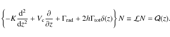
In this equation, N is the differential density of a given CR species,
- i)
- is the standard primary source term for sources located in
the thin disc. The quantity qs0
is the source abundance of nucleus j whose
source spectrum is
 .
.
- ii)
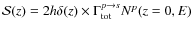
- is the standard secondary source term (also in the disc),
where
 is the production cross-section of nucleus p
into s. This simple form originates from
the straight-ahead approximation used when dealing with nuclei (see,
e.g., Maurin
et al. 2001, for more details).
is the production cross-section of nucleus p
into s. This simple form originates from
the straight-ahead approximation used when dealing with nuclei (see,
e.g., Maurin
et al. 2001, for more details).
- iii)
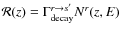
- described a contribution from a radioactive nucleus r, decaying into s' in both the disc and the halo.
A.1.1 Stable species
For a mixed species, primary and secondary standard sources add up,
so that, for a nucleus k
with no radioactive contribution, the source term is
rewritten as
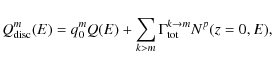
and the corresponding equation to solve is then

We find the solution in the halo, apply the boundary condition N(z=L)=0, and then ensure continuity between the disc and the halo, so that
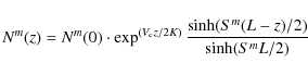
and
The quantities Sm and Am are defined as
|
(A.5) | |
|
(A.6) |
A.1.2
Adding a  -decay
source term: general solution
-decay
source term: general solution
It is emphasised in Maurin
et al. (2001) that the 10Be
![]() 10B
channel
contributes up to 10% in the secondary boron flux at low
energy and cannot be neglected. Although the spatial distribution of a
radioactive nucleus decreases exponentially with z,
we have to consider that the source term is emitted from the halo,
complicating the solution. The equation to solve for the
nucleus j, which is
10B
channel
contributes up to 10% in the secondary boron flux at low
energy and cannot be neglected. Although the spatial distribution of a
radioactive nucleus decreases exponentially with z,
we have to consider that the source term is emitted from the halo,
complicating the solution. The equation to solve for the
nucleus j, which is ![]() -fed by its radioactive
parent r is
-fed by its radioactive
parent r is

where Nr(z,E) is given by Eq. (A.3). The solution is found following the same steps as above, although it has a more complicated form (due to a non-vanishing source term in the halo).
If we take into account both the standard source term ![]() and the radioactive contribution of the nucleus Nr,
we obtain:
and the radioactive contribution of the nucleus Nr,
we obtain:
where
|
(A.8) |
and

![$\displaystyle \times ~\left\{ \frac{\nu a_i}{\cosh(S^jL/2)}\left[V_{\rm c} + 2h\Gamma^j \right] \right.$](/articles/aa/full_html/2010/08/aa14010-10/img240.png)
![$\displaystyle - ~\sinh(S^rL/2)\left[a\left( V_{\rm c}\left(2-\frac{K^j}{K^r}\right) + 2h\Gamma^j\right) +a_i K^jS^r\right]$](/articles/aa/full_html/2010/08/aa14010-10/img241.png)
![$\displaystyle \left. - ~ \cosh(S^rL/2)\left[a_i\left( V_{\rm c}\left(2-\frac{K^j}{K^r}\right) + 2h\Gamma^j\right) +a K^jS^r\right] \right\},$](/articles/aa/full_html/2010/08/aa14010-10/img242.png)
where


The superscript on K indicates that the diffusion coefficient is to be evaluated at a rigidity calculated for the nucleus m. The latter can differ from one nucleus to another because, the calculation is performed at the same kinetic energy per nucleon for all the nuclei (hence at slightly different rigidities for different nuclei). To compare with the data, the flux is calculated at z=0
![\begin{displaymath}%
N^j(0) = \varpi + \Theta \left[ \lambda\sinh \left(\frac{S^...
...{2}\right)
- \frac{\nu \Lambda}{\cosh \frac{S^jL}{2}} \right].
\end{displaymath}](/articles/aa/full_html/2010/08/aa14010-10/img245.png)
A.1.3 Solution including energy redistributions
When energy redistributions are included, the solution Nh(z)
in the halo remains the same because our model assumes no energy
redistributions in that region. Only the last step of the calculation
changes (ensuring continuity during the disc crossing). The new
solution is denoted
![]() .
.
For the case of a mixed species m without
radioactive contribution, the result is straightforward:
the solution for the halo is still given by Eq. (A.3),
but
![]() is now given by
is now given by

which is solved numerically, Nm(0) being the solution when energy terms are discarded, i.e., Eq. (A.4). The terms a(E) and b(E) describing energy losses and gains are discussed in Sect. 2.1.
When a radioactive contribution exists, the constant left to
determine is ![]() from Eq. (A.7),
which we denote now
from Eq. (A.7),
which we denote now ![]()
As above,
![\begin{displaymath}%
\Xi \equiv \Theta \left[ \lambda\sinh (\frac{S^rL}{2}) + \L...
...right)
- \frac{\nu \Lambda}{\cosh \frac{S^jL}{2}} \right]\cdot
\end{displaymath}](/articles/aa/full_html/2010/08/aa14010-10/img253.png)
|
(A.12) |
Hence

which we solve numerically.
This is the solution in the disc (z=0). The
solution for any z is obtained from
Eq. (A.7),
making the substitution
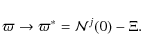
|
(A.13) |
We note that for
A.2 2D geometry
Cylindrical symmetry is now assumed, both the CR density N
and the source terms depending on r.
Compared to Eq. (A.1),
the operator
![]() now acts on N(r,z).
now acts on N(r,z).
An expansion along the first order Bessel function is
performed
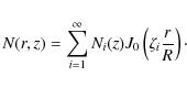
The quantity

so that each Bessel coefficient Ni(z) follows an equation very similar to Eq. (A.1), where

and where each source term must also be expanded on the Bessel basis. More details can be found in Maurin et al. (2001).
The full solutions for mixed species, with stable or
radioactive parents, is straightforwardly obtained from 1D
ones, after making the substitutions
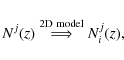
|
(A.15) |
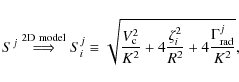
|
(A.16) |
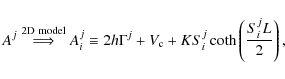
|
(A.17) |
and
|
(A.18) |
|
(A.19) |
|
(A.20) |
The above formulae, for the radioactive source, differ slightly from those presented in Maurin et al. (2001). However, the only difference is in the flux for
Appendix B: The local bubble
The underdensity in the local interstellar matter (LISM) is coined the
local bubble![]() . The LISM is a region of
extremely hot gas (
. The LISM is a region of
extremely hot gas (
![]() K) and low density (n
K) and low density (n ![]() 0.005 cm-3) within an asymmetric bubble
of radius
0.005 cm-3) within an asymmetric bubble
of radius ![]() 65-250 pc
surrounded by dense neutral hydrogen walls
(Redfield
& Linsky 2000; Sfeir et al. 1999;
Linsky
et al. 2000). This picture has been
refined by subsequent studies, e.g., Lallement
et al. (2003). The Sun is located inside a local
interstellar cloud (LIC) of typical extension
65-250 pc
surrounded by dense neutral hydrogen walls
(Redfield
& Linsky 2000; Sfeir et al. 1999;
Linsky
et al. 2000). This picture has been
refined by subsequent studies, e.g., Lallement
et al. (2003). The Sun is located inside a local
interstellar cloud (LIC) of typical extension ![]() pc whose density
pc whose density ![]()
![]() 0.1 cm-3 (Redfield & Falcon 2008;
Gloeckler
et al. 2004). Despite these successes, a complete
mapping and understanding of the position and properties of the
gas/cloudlets filling the LISM, as well as the issue of
interfaces with other bubbles remains challenging (e.g., Redfield
& Linsky 2008; Reis & Corradi 2008).
Based on existing data, numerical simulations of the local bubble infer
that it is the result of 14-19 SNe occurring in a moving
group, which passed through the present day local H
0.1 cm-3 (Redfield & Falcon 2008;
Gloeckler
et al. 2004). Despite these successes, a complete
mapping and understanding of the position and properties of the
gas/cloudlets filling the LISM, as well as the issue of
interfaces with other bubbles remains challenging (e.g., Redfield
& Linsky 2008; Reis & Corradi 2008).
Based on existing data, numerical simulations of the local bubble infer
that it is the result of 14-19 SNe occurring in a moving
group, which passed through the present day local H![]() cavity
13.5-14.5 Myr ago (Breitschwerdt & de
Avillez 2006). The same study suggests that the local bubble
expanded into the Milky Way halo roughly
5 Myr ago.
cavity
13.5-14.5 Myr ago (Breitschwerdt & de
Avillez 2006). The same study suggests that the local bubble
expanded into the Milky Way halo roughly
5 Myr ago.
A last important point, is that of the existence of turbulence in the LISM to scatter off CRs. The impact of the underdense local bubble on the production of radioactive nuclei as modelled in Eq. (10) depends whether the transport of the radioactive nuclei in this region is diffusive or not. In a study based on a measurement of the radio scintillation of a pulsar located within the local bubble, Spangler (2008) infers that values for the line of sight component of the magnetic field are only slightly less, or completely consistent with, lines of sight through the general interstellar medium; the turbulence is unexpectedly high in this region.
These pieces of observational evidences support the model used in Sect. 2.3, leading to an enhanced decrease in the flux of radioactive species at low energy. A detailed study should take into account the exact morphology of the ISM (asymmetry, cloudlets). However, there are so many uncertainties in this distribution and the associated level of turbulence, that a crude description is enough to capture a possible effect in the CR data.
Appendix C: MCMC optimisation
The efficiency of the MCMC increases when the PDFs of the parameters are close to resembling Gaussians. Large tails in PDFs require more steps to be sampled correctly. A usual task in the MCMC machinery is to find some combinations of parameters that ensure that these tails disappear. This was not discussed in the case of the LBM as the efficiency of the PDF calculation was satisfactory. In 1D (or 2D) DMs, the computing time is longer and the efficiency is found to be lower. To optimise and speed up the calculation, we provide combinations of parameters that correspond to a Gaussian distribution.
![\begin{figure}
\par\includegraphics[width=17cm,clip]{aa14010-figC1.eps}
\end{figure}](/articles/aa/full_html/2010/08/aa14010-10/img278.png)
|
Figure C.1:
Posterior PDFs of the model parameters (using the Binary Space
Partitioning step - see Paper I, and the
B/C constraint). The diagonals show the 1D marginalised PDF of
the indicated parameters, and the red line results from a Gaussian fit
to the histogram. Off-diagonal plots show the 2D marginalised
posterior PDFs for the parameters in the same column and same line,
respectively. The colour code corresponds to the regions of increasing
probability (from paler to darker shades), and the two contours
(smoothed) delimit regions containing respectively 68%
and 95% (inner and outer contour) of the PDF. Left
panel: PDFs for |
| Open with DEXTER | |
A typical PDF determination with four free parameters ![]() (see next section) is shown in Fig. C.1. The
diagonal of the left panel shows the PDF of these parameters (black
histogram), on which a Gaussian fit is superimposed (red
line). We see a sizeable tail for the K0 parameter,
and a small asymmetry for the
(see next section) is shown in Fig. C.1. The
diagonal of the left panel shows the PDF of these parameters (black
histogram), on which a Gaussian fit is superimposed (red
line). We see a sizeable tail for the K0 parameter,
and a small asymmetry for the ![]() parameter. The right
panel shows the same PDFs, but for the following combinations of the
transport parameters:
parameter. The right
panel shows the same PDFs, but for the following combinations of the
transport parameters:
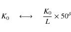
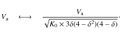
These forms are inspired by the known degeneracies between parameters. For instance, in diffusion models, the secondary to primary ratio is expected to remain unchanged as long as the effective grammage
A last combination is for the local bubble parameter ![]() :
:
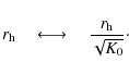
This comes from the form of Eq. (10), where the flux damping for radioactive species (due to the local bubble) is effective only at low energy (
Appendix D: Datasets for CR measurements
D.1 B/C ratio
Unless specified otherwise, the reference B/C dataset used throughout the paper is denoted dataset F: it consists of i) low-energy data taken by the IMP7-8 (Garcia-Munoz et al. 1987), the Voyager 1&2 (Lukasiak et al. 1999), and the ACE-CRIS (de Nolfo et al. 2006) spacecrafts; ii) intermediate energies acquired by HEA0-3 data (Engelmann et al. 1990); and iii) higher energy data from Spacelab (Swordy et al. 1990) and the published CREAM data (Ahn et al. 2008). Other existing data are discarded either because of their too large error bars, or because of their inconsistency with the above data (see Paper I).
D.2 Isotopic and elemental ratios of radioactive species
For 10Be/9Be, the data are taken from balloon flights (Buffington et al. 1978; Hagen et al. 1977; Webber & Kish 1979), including the ISOMAX balloon-borne instrument (Hams et al. 2004), and from the IMP-7/8 (Garcia-Munoz et al. 1977), ISEE-3 (Wiedenbeck & Greiner 1980), Ulysses (Connell 1998), Voyager (Lukasiak et al. 1999), and ACE spacecrafts (Yanasak et al. 2001). For 26Al/27Al, the data consist of a series of balloon flights (Webber 1982), and the ISEE-3 (Wiedenbeck 1983), Voyager (Lukasiak et al. 1994), Ulysses (Simpson & Connell 1998), and ACE spacecrafts (Yanasak et al. 2001). For 36Cl/Cl, the data are from the CRISIS balloon (Young et al. 1981), and from the Ulysses (Connell et al. 1998) and ACE (Yanasak et al. 2001) spacecrafts.
The data for the elemental ratios come from the HEAO-3 (Engelmann et al. 1990), Ulysses (Duvernois & Thayer 1996), and the ACE spacecrafts de Nolfo et al. (2006). The published ACE data on Al/Mg and Cl/Ar (George et al. 2009) were not used as Be/B is not provided.
References
- Abdo, A. A., Allen, B., Aune, T., et al. 2008, ApJ, 688, 1078 [Google Scholar]
- Abdo, A. A., Ackermann, M., Ajello, M., et al. 2009, Phys. Rev. Lett., 102, 1101 [Google Scholar]
- Adriani, O., Barbarino, G. C., Bazilevskaya, G. A., et al. 2009a, Nature, 458, 607 [CrossRef] [PubMed] [Google Scholar]
- Adriani, O., Barbarino, G. C., Bazilevskaya, G. A., et al. 2009b, Phys. Rev. Lett., 102, 051101 [NASA ADS] [CrossRef] [PubMed] [Google Scholar]
- Aglietta, M., Alekseenko, V. V., Alessandro, B., et al. 2009, ApJ, 692, L130 [Google Scholar]
- Aharonian, F., Akhperjanian, A. G., Bazer-Bachi, A. R., et al. 2006, Nature, 439, 695 [NASA ADS] [CrossRef] [PubMed] [Google Scholar]
- Aharonian, F., Akhperjanian, A. G., Barres de Almeida, U., et al. 2008, Phys. Rev. Lett., 101, 261104 [Google Scholar]
- Aharonian, F., Akhperjanian, A. G., Anton, G., et al. 2009, A&A, 508, 561 [NASA ADS] [CrossRef] [EDP Sciences] [Google Scholar]
- Ahn, H. S., Allison, P. S., Bagliesi, M. G., et al. 2008, Astrop. Phys., 30, 133 [NASA ADS] [CrossRef] [Google Scholar]
- Amenomori, M., Ayabe, S., Bi, X. J., et al. 2006, Science, 314, 439 [NASA ADS] [CrossRef] [PubMed] [Google Scholar]
- Anderson, L. D., & Bania, T. M. 2009, ApJ, 690, 706 [NASA ADS] [CrossRef] [Google Scholar]
- Ave, M., Boyle, P. J., Gahbauer, F., et al. 2008, ApJ, 678, 262 [Google Scholar]
- Berezhko, E. G., Ksenofontov, L. T., Ptuskin, V. S., Zirakashvili, V. N., & Völk, H. J. 2003, A&A, 410, 189 [NASA ADS] [CrossRef] [EDP Sciences] [Google Scholar]
- Berezinskii, V. S., Bulanov, S. V., Dogiel, V. A., & Ptuskin, V. S. 1990, Astrophysics of cosmic rays, ed. V. L. Ginzburg (Amsterdam: North-Holland) [Google Scholar]
- Berkhuijsen, E. M., & Müller, P. 2008, A&A, 490, 179 [NASA ADS] [CrossRef] [EDP Sciences] [Google Scholar]
- Berkhuijsen, E. M., Mitra, D., & Mueller, P. 2006, Astron. Nachr., 327, 82 [NASA ADS] [CrossRef] [Google Scholar]
- Bloemen, J. B. G. M., Dogiel, V. A., Dorman, V. L., & Ptuskin, V. S. 1993, A&A, 267, 372 [NASA ADS] [Google Scholar]
- Breitschwerdt, D., & de Avillez, M. A. 2006, A&A, 452, L1 [NASA ADS] [CrossRef] [EDP Sciences] [Google Scholar]
- Buffington, A., Orth, C. D., & Mast, T. S. 1978, ApJ, 226, 355 [NASA ADS] [CrossRef] [Google Scholar]
- Case, G. L., & Bhattacharya, D. 1998, ApJ, 504, 761 [Google Scholar]
- Casse, F., Lemoine, M., & Pelletier, G. 2002, Phys. Rev. D, 65, 023002 [Google Scholar]
- Castellina, A., & Donato, F. 2005, Astrop. Phys., 24, 146 [Google Scholar]
- Chang, J., Adams, J. H., Ahn, H. S., et al. 2008, Nature, 456, 362 [NASA ADS] [CrossRef] [PubMed] [Google Scholar]
- Choutko, V., & Giovacchini, F. 2008, 4, 765 [Google Scholar]
- Connell, J. J. 1998, ApJ, 501, L59 [NASA ADS] [CrossRef] [Google Scholar]
- Connell, J. J., Duvernois, M. A., & Simpson, J. A. 1998, ApJ, 509, L97 [NASA ADS] [CrossRef] [Google Scholar]
- de Nolfo, G. A., Moskalenko, I. V., Binns, W. R., et al. 2006, Adv. Space Res., 38, 1558 [NASA ADS] [CrossRef] [Google Scholar]
- Delahaye, T., Lineros, R., Donato, F., Fornengo, N., & Salati, P. 2008, Phys. Rev. D, 77, 063527 [NASA ADS] [CrossRef] [Google Scholar]
- Delahaye, T., Donato, F., Fornengo, N., et al. 2009, A&A, 501, 821 [NASA ADS] [CrossRef] [EDP Sciences] [Google Scholar]
- Donato, F., Maurin, D., Salati, P., et al. 2001, ApJ, 563, 172 [NASA ADS] [CrossRef] [Google Scholar]
- Donato, F., Maurin, D., & Taillet, R. 2002, A&A, 381, 539 [NASA ADS] [CrossRef] [EDP Sciences] [Google Scholar]
- Donato, F., Fornengo, N., Maurin, D., Salati, P., & Taillet, R. 2004, Phys. Rev. D, 69, 063501 [NASA ADS] [CrossRef] [Google Scholar]
- Donato, F., Fornengo, N., & Maurin, D. 2008, Phys. Rev. D, 78, 043506 [NASA ADS] [CrossRef] [Google Scholar]
- Donato, F., Maurin, D., Brun, P., Delahaye, T., & Salati, P. 2009, Phys. Rev. Lett., 102, 071301 [Google Scholar]
- Duvernois, M. A., & Thayer, M. R. 1996, ApJ, 465, 982 [Google Scholar]
- Engelmann, J. J., Ferrando, P., Soutoul, A., Goret, P., & Juliusson, E. 1990, A&A, 233, 96 [NASA ADS] [Google Scholar]
- Evoli, C., Gaggero, D., Grasso, D., & Maccione, L. 2008, J. Cosmol. Astro-Part. Phys., 10, 18 [Google Scholar]
- Farahat, A., Zhang, M., Rassoul, H., & Connell, J. J. 2008, ApJ, 681, 1334 [NASA ADS] [CrossRef] [Google Scholar]
- Ferrando, P., Webber, W. R., Goret, P., et al. 1988, Phys. Rev. C, 37, 1490 [NASA ADS] [CrossRef] [Google Scholar]
- Ferrière, K. M. 2001, Rev. Mod. Phys., 73, 1031 [NASA ADS] [CrossRef] [Google Scholar]
- Fuke, H., Koglin, J. E., Yoshida, T., et al. 2008, Adv. Space Res., 41, 2056 [NASA ADS] [CrossRef] [Google Scholar]
- Garcia-Munoz, M., Mason, G. M., & Simpson, J. A. 1977, ApJ, 217, 859 [NASA ADS] [CrossRef] [Google Scholar]
- Garcia-Munoz, M., Simpson, J. A., Guzik, T. G., Wefel, J. P., & Margolis, S. H. 1987, ApJS, 64, 269 [NASA ADS] [CrossRef] [EDP Sciences] [Google Scholar]
- George, J. S., Lave, K. A., Wiedenbeck, M. E., et al. 2009, ApJ, 698, 1666 [Google Scholar]
- Gloeckler, G., Möbius, E., Geiss, J., et al. 2004, A&A, 426, 845 [NASA ADS] [CrossRef] [EDP Sciences] [Google Scholar]
- Gómez, G. C., Benjamin, R. A., & Cox, D. P. 2001, AJ, 122, 908 [NASA ADS] [Google Scholar]
- Guillian, G., Hosaka, J., Ishihara, K., et al. 2007, Phys. Rev. D, 75, 062003 [NASA ADS] [CrossRef] [Google Scholar]
- Hagen, F. A., Fisher, A. J., & Ormes, J. F. 1977, ApJ, 212, 262 [NASA ADS] [CrossRef] [Google Scholar]
- Halzen, F., Kappes, A., & Ó Murchadha, A. 2008, Phys. Rev. D, 78, 063004 [Google Scholar]
- Hams, T., Barbier, L. M., Bremerich, M., et al. 2004, ApJ, 611, 892 [NASA ADS] [CrossRef] [Google Scholar]
- Jones, F. C. 1979, ApJ, 229, 747 [NASA ADS] [CrossRef] [Google Scholar]
- Jones, F. C., Lukasiak, A., Ptuskin, V., & Webber, W. 2001, ApJ, 547, 264 [NASA ADS] [CrossRef] [Google Scholar]
- Lallement, R., Welsh, B. Y., Vergely, J. L., Crifo, F., & Sfeir, D. 2003, A&A, 411, 447 [EDP Sciences] [Google Scholar]
- Linsky, J. L., Redfield, S., Wood, B. E., & Piskunov, N. 2000, ApJ, 528, 756 [NASA ADS] [CrossRef] [Google Scholar]
- Lionetto, A. M., Morselli, A., & Zdravkovic, V. 2005, J. Cosmol. Astro-Part. Phys., 9, 10 [NASA ADS] [CrossRef] [Google Scholar]
- Lukasiak, A., McDonald, F. B., & Webber, W. R. 1994, ApJ, 430, L69 [NASA ADS] [CrossRef] [Google Scholar]
- Lukasiak, A., McDonald, F. B., & Webber, W. R. 1999, 3, 41 [Google Scholar]
- Mannheim, K., & Schlickeiser, R. 1994, A&A, 286, 983 [NASA ADS] [Google Scholar]
- Marcowith, A., Lemoine, M., & Pelletier, G. 2006, A&A, 453, 193 [NASA ADS] [CrossRef] [EDP Sciences] [Google Scholar]
- Maurin, D., Donato, F., Taillet, R., & Salati, P. 2001, ApJ, 555, 585 [NASA ADS] [CrossRef] [Google Scholar]
- Maurin, D., Taillet, R., & Donato, F. 2002, A&A, 394, 1039 [NASA ADS] [CrossRef] [EDP Sciences] [Google Scholar]
- Maurin, D., Taillet, R., & Combet, C. 2006 [arXiv:astro-ph/0612714] [Google Scholar]
- Maurin, D., Putze, A., & Derome, L. 2010, A&A, 516, A67 [NASA ADS] [CrossRef] [EDP Sciences] [Google Scholar]
- Minnie, J., Bieber, J. W., Matthaeus, W. H., & Burger, R. A. 2007, ApJ, 663, 1049 [NASA ADS] [CrossRef] [Google Scholar]
- Moskalenko, I. V., Mashnik, S. G., & Strong, A. W. 2001, 5, 1836 [Google Scholar]
- Nordgren, T. E., Cordes, J. M., & Terzian, Y. 1992, AJ, 104, 1465 [NASA ADS] [CrossRef] [Google Scholar]
- Osborne, J. L., & Ptuskin, V. S. 1988, SvA Lett., 14, 132 [Google Scholar]
- Panov, A. D., Sokolskaya, N. V., Adams, J. H., Jr., et al. 2008, 2, 3 [Google Scholar]
- Plaga, R. 2008, Nature, 453, 48 [NASA ADS] [CrossRef] [PubMed] [Google Scholar]
- Ptuskin, V. S., Jones, F. C., Ormes, J. F., & Soutoul, A. 1997, Adv. Space Res., 19, 787 [NASA ADS] [CrossRef] [Google Scholar]
- Ptuskin, V. S., Moskalenko, I. V., Jones, F. C., Strong, A. W., & Zirakashvili, V. N. 2006, ApJ, 642, 902 [NASA ADS] [CrossRef] [Google Scholar]
- Ptuskin, V. S., & Soutoul, A. 1990, A&A, 237, 445 [NASA ADS] [Google Scholar]
- Ptuskin, V. S., & Soutoul, A. 1998, A&A, 337, 859 [NASA ADS] [Google Scholar]
- Putze, A., Derome, L., Maurin, D., Perotto, L., & Taillet, R. 2009, A&A, 497, 991 [NASA ADS] [CrossRef] [EDP Sciences] [Google Scholar]
- Redfield, S., & Linsky, J. L. 2000, ApJ, 534, 825 [NASA ADS] [CrossRef] [Google Scholar]
- Redfield, S., & Falcon, R. E. 2008, ApJ, 683, 207 [NASA ADS] [CrossRef] [Google Scholar]
- Redfield, S., & Linsky, J. L. 2008, ApJ, 673, 283 [NASA ADS] [CrossRef] [Google Scholar]
- Reis, W., & Corradi, W. J. B. 2008, A&A, 486, 471 [NASA ADS] [CrossRef] [EDP Sciences] [Google Scholar]
- Reville, B., O'Sullivan, S., Duffy, P., & Kirk, J. G. 2008, MNRAS, 386, 509 [NASA ADS] [CrossRef] [Google Scholar]
- Reynolds, S. P. 2008, ARA&A, 46, 89 [Google Scholar]
- Seo, E. S., & Ptuskin, V. S. 1994, ApJ, 431, 705 [NASA ADS] [CrossRef] [Google Scholar]
- Sfeir, D. M., Lallement, R., Crifo, F., & Welsh, B. Y. 1999, A&A, 346, 785 [NASA ADS] [Google Scholar]
- Shibata, T., Hareyama, M., Nakazawa, M., & Saito, C. 2006, ApJ, 642, 882 [NASA ADS] [CrossRef] [Google Scholar]
- Silberberg, R., & Tsao, C. H. 1990, Phys. Rep., 191, 353 [Google Scholar]
- Simpson, J. A., & Connell, J. J. 1998, ApJ, 497, L85 [NASA ADS] [CrossRef] [Google Scholar]
- Spangler, S. R. 2008, Space Sci. Rev., 98 [Google Scholar]
- Strong, A. W., & Moskalenko, I. V. 1998, ApJ, 509, 212 [NASA ADS] [CrossRef] [Google Scholar]
- Strong, A. W., Moskalenko, I. V., & Ptuskin, V. S. 2007, Ann. Rev. Nucl. Part. Sci., 57, 285 [NASA ADS] [CrossRef] [Google Scholar]
- Swordy, S. P., Mueller, D., Meyer, P., L'Heureux, J., & Grunsfeld, J. M. 1990, ApJ, 349, 625 [NASA ADS] [CrossRef] [Google Scholar]
- Taillet, R., & Maurin, D. 2003, A&A, 402, 971 [NASA ADS] [CrossRef] [EDP Sciences] [Google Scholar]
- Tautz, R. C., Shalchi, A., & Schlickeiser, R. 2008, ApJ, 672, 642 [NASA ADS] [CrossRef] [Google Scholar]
- The Fermi-LAT Collaboration 2009, , 103, 251101 [Google Scholar]
- Tomassetti, N., & AMS-01 Collaboration 2009, in International Cosmic Ray Conference, 1 [Google Scholar]
- Torii, S., Yamagami, T., Tamura, T., et al. 2008, Astropart. Phys., submitted [arXiv:0809.0760] [Google Scholar]
- Uchiyama, Y., Aharonian, F. A., Tanaka, T., Takahashi, T., & Maeda, Y. 2007, Nature, 449, 576 [NASA ADS] [CrossRef] [PubMed] [Google Scholar]
- Webber, W. R. 1982, ApJ, 252, 386 [NASA ADS] [CrossRef] [Google Scholar]
- Webber, W. R. 1997, Space Sci. Rev., 81, 107 [NASA ADS] [CrossRef] [Google Scholar]
- Webber, W. R., & Kish, J. 1979, 1, 389 [Google Scholar]
- Webber, W. R., & Soutoul, A. 1998, ApJ, 506, 335 [NASA ADS] [CrossRef] [Google Scholar]
- Webber, W. R., Kish, J. C., & Schrier, D. A. 1990, Phys. Rev. C, 41, 566 [NASA ADS] [CrossRef] [Google Scholar]
- Webber, W. R., Lee, M. A., & Gupta, M. 1992, ApJ, 390, 96 [NASA ADS] [CrossRef] [Google Scholar]
- Webber, W. R., Kish, J. C., Rockstroh, J. M., et al. 1998, ApJ, 508, 940 [NASA ADS] [CrossRef] [Google Scholar]
- Webber, W. R., Soutoul, A., Kish, J. C., & Rockstroh, J. M. 2003, ApJS, 144, 153 [NASA ADS] [CrossRef] [Google Scholar]
- Wiedenbeck, M. E. 1983, in International Cosmic Ray Conference, 9, 147 [Google Scholar]
- Wiedenbeck, M. E., & Greiner, D. E. 1980, ApJ, 239, L139 [NASA ADS] [CrossRef] [Google Scholar]
- Yan, H., & Lazarian, A. 2008, ApJ, 673, 942 [NASA ADS] [CrossRef] [Google Scholar]
- Yanasak, N. E., Wiedenbeck, M. E., Mewaldt, R. A., et al. 2001, ApJ, 563, 768 [NASA ADS] [CrossRef] [Google Scholar]
- Young, J. S., Freier, P. S., Waddington, C. J., Brewster, N. R., & Fickle, R. K. 1981, ApJ, 246, 1014 [NASA ADS] [CrossRef] [Google Scholar]
Footnotes
- ... time
![[*]](/icons/foot_motif.png)
- The 2D solution is based on a Bessel expansion/resummation (see Eq. (A.14)). For each Bessel order, an equation similar to that for the 1D geometry needs to be solved. Nine Bessel orders are in many cases enough to ensure convergence (Maurin et al. 2001), but at least 100 orders are required in the general case, which multiply the computing time by roughly the same amount.
- ... package
- http://galprop.stanford.edu/web_galprop/galprop_home.html
- ... figure)
- The impact on the transport parameters is detailed in Sect. 7 of Maurin et al. (2010): the region of the best-fit values is slightly displaced, as seen in the figure.
- ... bubble
- For a state-of-the-art view on the subject, the reader is referred to the proceedings of a conference held in 2008: The Local Bubble and Beyond II - http://lbb.gsfc.nasa.gov/
All Tables
Table 1: Classes of models tested in the paper.
Table 2: Most probable values for B/C data only (L=4 kpc).
Table 3: Best-fit model parameters for B/C data only (L=4 kpc).
Table 4: Best-fit model parameters based on different B/C datasets.
Table 5: Best-fit parameters on B/C data for the LBM.
Table 6: Best-fit model parameters on B/C data: 1D versus 2D DM (L=4 kpc).
Table 7:
Most probable values for models II and III for the
free parameters of the local bubble radius ![]() and/or the Galactic halo size L
(constrained by B/C and 10Be/9Be data).
and/or the Galactic halo size L
(constrained by B/C and 10Be/9Be data).
Table 8: Best-fit parameters on B/C + 10Be/9Be26 + Al/27Al + 36Cl/Cl: 1D vs. 2D DM.
All Figures
| |
Figure 1:
Sketch of the model: sources and interactions (including energy losses
and gains) are restricted to the thin disc |
| Open with DEXTER | |
| In the text | |
|
|
Figure 2: From top to bottom: posterior PDFs of models I-III using the B/C constraint (dataset F). The diagonals show the 1D marginalised PDFs of the indicated parameters. Off-diagonal plots show the 2D marginalised posterior PDFs for the parameters in the same column and same line respectively. The colour code corresponds to the regions of increasing probability (from paler to darker shade), and the two contours (smoothed) delimit regions containing, respectively, 68% and 95% (inner and outer contour) of the PDF. |
| Open with DEXTER | |
| In the text | |
|
|
Figure 3:
Best-fit ratio for model I (blue-dotted line), II (red-dashed
line), and
model III (black-solid line) using dataset F: IMP7-8,
Voyager1&2, ACE-CRIS, HEAO-3, Spacelab, and CREAM. The curves
are modulated with |
| Open with DEXTER | |
| In the text | |
|
|
Figure 4:
B/C data used in this section. Shown are the IS data (rescaled
from TOA data using |
| Open with DEXTER | |
| In the text | |
|
|
Figure 5:
Best-fit parameters (III-F) as a function of the halo size of the
Galaxy (blue circles). From top to bottom: K0, |
| Open with DEXTER | |
| In the text | |
|
|
Figure 6:
Model II (diffusion/reacceleration): marginalised posterior PDF of the
diffusive halo size L (right panels
of the first and second row) and the local bubble radius |
| Open with DEXTER | |
| In the text | |
|
|
Figure 7:
Model III (diffusion/convection/reacceleration): same as in
Fig. 6.
The transport parameters are now |
| Open with DEXTER | |
| In the text | |
|
|
Figure 8:
Model II: marginalised posterior PDFs of the Galactic geometry
parameters for the standard DM (
|
| Open with DEXTER | |
| In the text | |
|
|
Figure 9: Same as in Fig. 8, but for model III. |
| Open with DEXTER | |
| In the text | |
|
|
Figure 10:
Shown are the envelopes of 68% CL (shaded areas) and best-fit
(thick lines) ratios for the standard DM II (
|
| Open with DEXTER | |
| In the text | |
|
|
Figure 11:
Left panel: standard DM model (
|
| Open with DEXTER | |
| In the text | |
|
|
Figure 12:
Best-fit value of the halo size L as a
function of |
| Open with DEXTER | |
| In the text | |
|
|
Figure 13: Same as in Fig. 10 but for the ratios Be/B, Al/Mg, and Cl/Ar. |
| Open with DEXTER | |
| In the text | |
|
|
Figure C.1:
Posterior PDFs of the model parameters (using the Binary Space
Partitioning step - see Paper I, and the
B/C constraint). The diagonals show the 1D marginalised PDF of
the indicated parameters, and the red line results from a Gaussian fit
to the histogram. Off-diagonal plots show the 2D marginalised
posterior PDFs for the parameters in the same column and same line,
respectively. The colour code corresponds to the regions of increasing
probability (from paler to darker shades), and the two contours
(smoothed) delimit regions containing respectively 68%
and 95% (inner and outer contour) of the PDF. Left
panel: PDFs for |
| Open with DEXTER | |
| In the text | |
Copyright ESO 2010
Current usage metrics show cumulative count of Article Views (full-text article views including HTML views, PDF and ePub downloads, according to the available data) and Abstracts Views on Vision4Press platform.
Data correspond to usage on the plateform after 2015. The current usage metrics is available 48-96 hours after online publication and is updated daily on week days.
Initial download of the metrics may take a while.