| Issue |
A&A
Volume 516, June-July 2010
|
|
|---|---|---|
| Article Number | A113 | |
| Number of page(s) | 6 | |
| Section | Astrophysical processes | |
| DOI | https://doi.org/10.1051/0004-6361/200913558 | |
| Published online | 22 July 2010 | |
Searching for spatial variations of
 in the Milky Way
S. A. Levshakov1,2,3 - P. Molaro1 - D. Reimers4
1 - INAF-Osservatorio Astronomico di Trieste, via G. B. Tiepolo 11,
34131 Trieste, Italy
2 -
Key Laboratory for Research in Galaxies and Cosmology,
Shanghai Astronomical Observatory, CAS, 80 Nandan Road, Shanghai 200030,
PR China
3 -
Ioffe Physical-Technical Institute,
Polytekhnicheskaya Str. 26, 194021 St. Petersburg, Russia
4 -
Hamburger Sternwarte, Universität Hamburg,
Gojenbergsweg 112, 21029 Hamburg, Germany
Received 27 October 2009 / Accepted 2 April 2010
Abstract
Aims. We probe the dependence of
![]() on the ambient matter density by means of spectral observations in submm- and mm-wave bands.
on the ambient matter density by means of spectral observations in submm- and mm-wave bands.
Methods. A procedure is suggested for exploring the value of
![]() ,
where
,
where
![]() is the electron-to-proton mass ratio, and
is the electron-to-proton mass ratio, and
![]() is the fine-structure constant. The fundamental physical constants,
which are measured in different physical environments of high
(terrestrial) and low (interstellar) densities of baryonic matter are
supposed to vary in chameleon-like scalar field models, which predict
that both masses and coupling constant may depend on the local matter
density. The parameter
is the fine-structure constant. The fundamental physical constants,
which are measured in different physical environments of high
(terrestrial) and low (interstellar) densities of baryonic matter are
supposed to vary in chameleon-like scalar field models, which predict
that both masses and coupling constant may depend on the local matter
density. The parameter
![]() can be estimated from the radial velocity offset,
can be estimated from the radial velocity offset,
![]() ,
between the low-laying rotational transitions in carbon monoxide 13CO and the fine-structure transitions in atomic carbon [C I]. A model-dependent constraint on
,
between the low-laying rotational transitions in carbon monoxide 13CO and the fine-structure transitions in atomic carbon [C I]. A model-dependent constraint on
![]() can be obtained from
can be obtained from
![]() using
using
![]() independently measured from the ammonia method.
independently measured from the ammonia method.
Results. Currently available radio astronomical datasets provide an upper limit on
![]() m s-1 (
m s-1 (![]() ). When interpreted in terms of the spatial variation of F, this gives
). When interpreted in terms of the spatial variation of F, this gives
![]() .
An order of magnitude improvement in this limit will allow us to independently test a non-zero value of
.
An order of magnitude improvement in this limit will allow us to independently test a non-zero value of
![]() =
=
![]() ,
recently found with the ammonia method. Considering that the ammonia method restricts the spatial variation of
,
recently found with the ammonia method. Considering that the ammonia method restricts the spatial variation of ![]() at the level of
at the level of
![]() and assuming that
and assuming that
![]() is the same in the entire interstellar medium, one obtains that the spatial variation of
is the same in the entire interstellar medium, one obtains that the spatial variation of ![]() does not exceed the value
does not exceed the value
![]() .
Since extragalactic gas clouds have similar densities to those in the interstellar medium, the bound on
.
Since extragalactic gas clouds have similar densities to those in the interstellar medium, the bound on
![]() is also expected to be less than
is also expected to be less than
![]() at high redshift if no significant temporal dependence of
at high redshift if no significant temporal dependence of ![]() is present.
is present.
Key words: line: profiles - ISM: molecules - techniques: radial velocities - cosmology: observations
1 Introduction
The dimensionless physical constants, such as
the electron-to-proton mass ratio,
![]() ,
or the fine-structure constant,
,
or the fine-structure constant,
![]() ,
are expected to be dynamical quantities in modern extensions of
the standard model of particle physics
(Uzan 2003; Garcia-Berro et al. 2007; Martins 2008; Kanekar 2008; Chin et al. 2009).
Exploring these predictions is a subject of many high-precision measurements
in contemporary laboratory and astrophysical experiments.
The most accurate laboratory constraints on temporal
,
are expected to be dynamical quantities in modern extensions of
the standard model of particle physics
(Uzan 2003; Garcia-Berro et al. 2007; Martins 2008; Kanekar 2008; Chin et al. 2009).
Exploring these predictions is a subject of many high-precision measurements
in contemporary laboratory and astrophysical experiments.
The most accurate laboratory constraints on temporal ![]() - and
- and ![]() -variations
of
-variations
of
![]() yr-1,
and
yr-1,
and
![]() yr-1
have been obtained by Rosenband et al. (2008), and
Blatt et al. (2008), respectively.
yr-1
have been obtained by Rosenband et al. (2008), and
Blatt et al. (2008), respectively.
For the monotonic dependence of ![]() and
and ![]() on cosmic time,
at redshift
on cosmic time,
at redshift ![]() (corresponding look-back time is
(corresponding look-back time is
![]() yr)
the changes in
yr)
the changes in ![]() and
and ![]() would be restricted at the level of
would be restricted at the level of
![]() and
and
![]() .
Here,
.
Here,
![]() (or
(or
![]() )
is a fractional change in
)
is a fractional change in ![]() between a reference value
between a reference value ![]() and
a given measurement
and
a given measurement ![]() obtained at different epochs or at different spatial coordinates:
obtained at different epochs or at different spatial coordinates:
![]() .
.
These constraints are in line with geological measurements of
relative isotopic abundances in the Oklo natural fission reactor,
which allows us to probe ![]() at
at
![]() yr (
yr (
![]() ).
Assuming possible changes only in the electromagnetic coupling constant, Gould et al. (2006)
has obtained a model dependent constraint on
).
Assuming possible changes only in the electromagnetic coupling constant, Gould et al. (2006)
has obtained a model dependent constraint on
![]() .
However, when the strength of the strong interaction - the parameter
.
However, when the strength of the strong interaction - the parameter
![]() -
is also considered to be variable, the Oklo data does not provide any bound on
the variation of
-
is also considered to be variable, the Oklo data does not provide any bound on
the variation of ![]() (Flambaum & Shuryak 2002; Chin et al. 2009).
(Flambaum & Shuryak 2002; Chin et al. 2009).
Current astrophysical measurements at higher redshifts are as follows.
There was a claim for a variability in ![]() at
the 5
at
the 5![]() confidence level:
confidence level:
![]() ppm
(Murphy et al. 2004)
ppm
(Murphy et al. 2004)![]() ,
but this has not been confirmed in other measurements that led to the upper bound
,
but this has not been confirmed in other measurements that led to the upper bound
![]() ppm (Quast et al. 2004;
Levshakov et al. 2005; Srianand et al. 2008; Molaro et al. 2008).
ppm (Quast et al. 2004;
Levshakov et al. 2005; Srianand et al. 2008; Molaro et al. 2008).
Measurements of the cosmological ![]() -variation exhibit a similar tendency.
Non-zero values of
-variation exhibit a similar tendency.
Non-zero values of
![]() ppm,
ppm,
![]() ppm
(Ivanchik et al. 2005), and
ppm
(Ivanchik et al. 2005), and
![]() ppm
(Reinhold et al. 2006) found at z = 2.595 (Q 0405-443) and z = 3.025 (Q 0347-383)
from the Werner and Lyman bands of H2were later refuted by Wendt & Reimers (2008), King et al. (2008)
and Thompson et al. (2009), who used the same optical absorption-line spectra of quasars
and restricted changes in
ppm
(Reinhold et al. 2006) found at z = 2.595 (Q 0405-443) and z = 3.025 (Q 0347-383)
from the Werner and Lyman bands of H2were later refuted by Wendt & Reimers (2008), King et al. (2008)
and Thompson et al. (2009), who used the same optical absorption-line spectra of quasars
and restricted changes in ![]() at the level of
at the level of
![]() ppm.
The third H2 system at z = 2.059 towards the quasar J2123-0050 also
does not show any evidence of cosmological variation in
ppm.
The third H2 system at z = 2.059 towards the quasar J2123-0050 also
does not show any evidence of cosmological variation in ![]() :
:
![]() ppm (Malec et al. 2010).
More stringent constraints have been obtained at lower redshifts
from radio observations of the absorption lines of NH3 and other molecules:
ppm (Malec et al. 2010).
More stringent constraints have been obtained at lower redshifts
from radio observations of the absorption lines of NH3 and other molecules:
![]() ppm at z = 0.68 (Murphy et al. 2008), and
ppm at z = 0.68 (Murphy et al. 2008), and
![]() ppm at z = 0.89 (Henkel et al. 2009).
Two cool gas absorbers at z = 1.36 (Q 2337-011) and z = 1.56 (Q 0458-020)
have recently been studied in the H I 21cm and C I
ppm at z = 0.89 (Henkel et al. 2009).
Two cool gas absorbers at z = 1.36 (Q 2337-011) and z = 1.56 (Q 0458-020)
have recently been studied in the H I 21cm and C I
![]() absorption lines providing a constraint on the variation in the product
absorption lines providing a constraint on the variation in the product
![]() (here
(here ![]() is the proton gyromagnetic ratio):
is the proton gyromagnetic ratio):
![]() ppm (Kanekar et al. 2010).
Thus, the most accurate astronomical estimates restrict cosmological
variations in the fundamental physical constants at the level of
ppm (Kanekar et al. 2010).
Thus, the most accurate astronomical estimates restrict cosmological
variations in the fundamental physical constants at the level of ![]() 1-2 ppm.
1-2 ppm.
The estimate of fractional changes in
![]() and
and
![]() by
spectral methods is always a measurement of the relative Doppler shifts between
the line centers of different atoms/molecules
and their comparison with corresponding laboratory values
(Savedoff 1956; Bahcall et al. 1967; Wolfe et al. 1976; Dzuba 1999, 2002; Levshakov 2004;
Kanekar & Chengalur 2004).
To distinguish the line shifts due to radial motion of the object from those caused by
the variability in constants, lines with different
sensitivity coefficients,
by
spectral methods is always a measurement of the relative Doppler shifts between
the line centers of different atoms/molecules
and their comparison with corresponding laboratory values
(Savedoff 1956; Bahcall et al. 1967; Wolfe et al. 1976; Dzuba 1999, 2002; Levshakov 2004;
Kanekar & Chengalur 2004).
To distinguish the line shifts due to radial motion of the object from those caused by
the variability in constants, lines with different
sensitivity coefficients, ![]() ,
to the variations of
,
to the variations of ![]() and/or
and/or ![]() are to be used
are to be used![]() .
It is clear that the greater the difference
.
It is clear that the greater the difference
![]() between two transitions, the higher the accuracy of such estimates.
between two transitions, the higher the accuracy of such estimates.
Optical and UV transitions in atoms, ions, and
molecular hydrogen H2 have similar
sensitivity coefficients with
![]() not exceeding 0.05
(Varshalovich & Levshakov 1993; Dzuba 1999, 2002; Porsev et al. 2007).
For atomic spectra, the estimate of
not exceeding 0.05
(Varshalovich & Levshakov 1993; Dzuba 1999, 2002; Porsev et al. 2007).
For atomic spectra, the estimate of
![]() is given
in linear approximation (
is given
in linear approximation (
![]() )
by (e.g., Levshakov et al. 2006):
)
by (e.g., Levshakov et al. 2006):
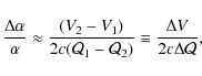
where V1, V2 are the radial velocities of two atomic lines, and c the speed of light. It was shown in Molaro et al. (2008) that the limiting accuracy of the wavelength scale calibration for the VLT/UVES quasar spectra at any point within the whole optical domain is about 30 m s-1 , which corresponds to the limiting relative accuracy between two lines measured in different parts of the same spectrum of about 50 m s-1 . Considering that
A considerably higher sensitivity to the variation in physical constants
is observed in radio range.
For example, van Veldhoven et al. (2004) first showed that
the inversion frequency of the
(J,K) = (1,1) level of
the ammonia isotopologue 15ND3 has the sensitivity coefficient
![]() .
Compared to optical and UV transitions,
the ammonia method proposed by Flambaum & Kozlov (2007)
provides 35 times more sensitive an estimate of
.
Compared to optical and UV transitions,
the ammonia method proposed by Flambaum & Kozlov (2007)
provides 35 times more sensitive an estimate of
![]() from measurements of the radial velocity offset between
the NH3
(J,K) = (1,1) inversion transition at 23.7 GHz and
low-lying rotational transitions of other molecules co-spatially distributed with
NH3:
from measurements of the radial velocity offset between
the NH3
(J,K) = (1,1) inversion transition at 23.7 GHz and
low-lying rotational transitions of other molecules co-spatially distributed with
NH3:
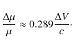
The ammonia method was recently used to explore possible spatial variations
In the present paper we consider fractional changes in a combination of two constants
![]() and
and ![]() ,
,
![]() ,
which are estimated from the comparison of transition frequencies
measured in different physical environments of
high (terrestrial) and low (interstellar) densities of baryonic matter.
The idea behind this experiment is that some class of scalar field models -
so-called chameleon-like fields - predict the dependence
of both masses and coupling constant on the local matter density
(Olive & Pospelov 2008).
Chameleon-like scalar fields have been introduced by
Khoury & Weltman (2004a,b) and by Brax et al. (2004)
to explain negative results on laboratory searches for the fifth force,
which should arise inevitably from couplings between scalar fields and
standard model particles.
The chameleon models assume that a light scalar field acquires both an effective potential
and effective mass because of its coupling to matter that depends on the
ambient matter density.
,
which are estimated from the comparison of transition frequencies
measured in different physical environments of
high (terrestrial) and low (interstellar) densities of baryonic matter.
The idea behind this experiment is that some class of scalar field models -
so-called chameleon-like fields - predict the dependence
of both masses and coupling constant on the local matter density
(Olive & Pospelov 2008).
Chameleon-like scalar fields have been introduced by
Khoury & Weltman (2004a,b) and by Brax et al. (2004)
to explain negative results on laboratory searches for the fifth force,
which should arise inevitably from couplings between scalar fields and
standard model particles.
The chameleon models assume that a light scalar field acquires both an effective potential
and effective mass because of its coupling to matter that depends on the
ambient matter density.
In this way, the chameleon
scalar field may evade local tests of the equivalence principle and fifth force experiments,
since the range of the scalar-mediated fifth force for the terrestrial
matter densities is too narrow to be detected.
Similarly, laboratory tests with atomic clocks for ![]() -variations
are performed under conditions of constant local density, so
they are not sensitive to the presence of the chameleon scalar field (Upadhye et al. 2010).
This is not the case for space-based tests, where the matter density is considerably lower,
an effective mass of the scalar field is negligible,
and an effective range for the scalar-mediated force is broad.
Light scalar fields are usually attributed to a negative pressure substance
permeating the entire visible Universe and known as dark energy (Caldwell et al. 1998).
This substance is thought to be responsible
for a cosmic acceleration at low redshifts,
-variations
are performed under conditions of constant local density, so
they are not sensitive to the presence of the chameleon scalar field (Upadhye et al. 2010).
This is not the case for space-based tests, where the matter density is considerably lower,
an effective mass of the scalar field is negligible,
and an effective range for the scalar-mediated force is broad.
Light scalar fields are usually attributed to a negative pressure substance
permeating the entire visible Universe and known as dark energy (Caldwell et al. 1998).
This substance is thought to be responsible
for a cosmic acceleration at low redshifts, ![]() (Peebles & Rata 2003; Brax 2009).
(Peebles & Rata 2003; Brax 2009).
2 [C I] and CO lines as probes of

The variations in the physical constants can be probed through atomic fine-structure (FS) and molecular rotational transitions (Levshakov et al. 2008; Kozlov et al. 2008). The corresponding lines are observed in submm- and mm-wavelength ranges. Along with a gain in sensitivity, using such transitions allows us to estimate constants at very high redshifts (z > 5) that are inaccessible to optical observations.
Let us consider radial velocity offsets between molecular
rotational and atomic FS lines,
![]() .
The offset
.
The offset ![]() is related to the parameter
is related to the parameter
![]() as follows (Levshakov et al. 2008):
as follows (Levshakov et al. 2008):
The velocity offset in Eq. (3) can be represented by the sum of two components
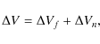
where
The Doppler noise yields offsets that can either mimic or obliterate a real signal.
Nevertheless, if these offsets are random, the
signal
![]() can be estimated statistically by
averaging over a large data sample:
can be estimated statistically by
averaging over a large data sample:
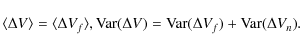
Here we assume that the noise component has a zero mean and a finite variance.
The Doppler noise component can be minimized if the chosen species are
closely trace each other. An appropriate pair in our case is the
atomic carbon FS transitions and rotational transitions of carbon monoxide 13CO.
The spatial distributions of 13CO and
[C I] are known to be well correlated
(Keene et al. 1985; Meixner & Tielens 1995; Spaans & van Dishoeck 1997;
Ikeda et al. 2002; Papadopoulos et al. 2004).
The carbon-bearing species C0, C+, and CO are observed in photodissociation
regions (PDRs) - neutral regions where chemistry and heating are regulated
by the far-UV photons (Hollenbach & Tielens 1999).
The PDR is either the interface between the H II region and the molecular
cloud or a neutral component of the diffuse interstellar medium (ISM).
Far-UV photons (6.0 eV
![]() eV) are produced by OB stars.
Photons with energy greater than 11.1 eV dissociate CO into atomic carbon and oxygen.
Since the C0 ionization potential of 11.3 eV is quite close to the CO
dissociation energy, neutral carbon can be quickly ionized. This suggests the chemical
stratification of the PDR in the line C+/C0/CO with increasing depth from
the surface of the PDR. Then, one can assume that, in the outer envelopes
of molecular clouds, neutral carbon lies within a thin layer determined by the
equilibrium between photoionization/recombination processes on the C+/C0 side
and photodissociation/molecule formation processes on the C0/CO side.
However, observations (Keene et al. 1985; Zhang et al. 2001)
do not support such a steady-state model, which predicts that
C0 should only arise near the edges of molecular clouds.
To explain the observed correlation between the spatial distributions of
C0 and CO, inhomogeneous PDRs with clumping molecular gas were suggested.
The revealed ubiquity of the [C I] transition
eV) are produced by OB stars.
Photons with energy greater than 11.1 eV dissociate CO into atomic carbon and oxygen.
Since the C0 ionization potential of 11.3 eV is quite close to the CO
dissociation energy, neutral carbon can be quickly ionized. This suggests the chemical
stratification of the PDR in the line C+/C0/CO with increasing depth from
the surface of the PDR. Then, one can assume that, in the outer envelopes
of molecular clouds, neutral carbon lies within a thin layer determined by the
equilibrium between photoionization/recombination processes on the C+/C0 side
and photodissociation/molecule formation processes on the C0/CO side.
However, observations (Keene et al. 1985; Zhang et al. 2001)
do not support such a steady-state model, which predicts that
C0 should only arise near the edges of molecular clouds.
To explain the observed correlation between the spatial distributions of
C0 and CO, inhomogeneous PDRs with clumping molecular gas were suggested.
The revealed ubiquity of the [C I] transition
![]()
![]() in molecular clouds agrees with
clumpy PDR models (Meixner & Tielens 1995; Spaans et al. 1997;
Papadopoulos et al. 2004).
in molecular clouds agrees with
clumpy PDR models (Meixner & Tielens 1995; Spaans et al. 1997;
Papadopoulos et al. 2004).
The ground state of the C0 atom consists of the
3P1,2,3 triplet levels.
The energies of the fine-structure excited levels relative to the ground state
are
E0,1 = 24 K and
E0,2 = 63 K, and the transition
probabilities are
![]() s-1 and
s-1 and
![]() s-1 (Silva & Viegas 2002).
The excitation rates of the [C I] J = 1 and J = 2 levels for
collisions with H2 at
s-1 (Silva & Viegas 2002).
The excitation rates of the [C I] J = 1 and J = 2 levels for
collisions with H2 at
![]() K are
K are
![]() cm3 s-1 (Schröder et al. 1991).
This implies that for the J = 1 and J = 2 levels the critical densities
are 1000 cm-3 and 3000 cm-3 , respectively. The low-J rotational transitions
of CO trace similar moderately dense (
cm3 s-1 (Schröder et al. 1991).
This implies that for the J = 1 and J = 2 levels the critical densities
are 1000 cm-3 and 3000 cm-3 , respectively. The low-J rotational transitions
of CO trace similar moderately dense (
![]() cm-3 ) and cold (
cm-3 ) and cold (
![]() K)
gas. It is not completely excluded, however, that
some heterogeneity of spatial distributions of [C I] and 13CO may occur,
resulting in the radial velocity offsets.
K)
gas. It is not completely excluded, however, that
some heterogeneity of spatial distributions of [C I] and 13CO may occur,
resulting in the radial velocity offsets.
In the chameleon-like scalar field models for density-dependent ![]() and
and
![]() ,
the fractional changes in these constants arise from the shift in the expectation value
of the scalar field between high and low density environments.
Since the matter density in the interstellar clouds is
,
the fractional changes in these constants arise from the shift in the expectation value
of the scalar field between high and low density environments.
Since the matter density in the interstellar clouds is ![]() 1016 times
lower than in terrestrial environments, whereas
gas densities between the molecular clouds themselves are much lower
(
1016 times
lower than in terrestrial environments, whereas
gas densities between the molecular clouds themselves are much lower
(
![]() cm-3 ),
all interstellar clouds
can be considered as having similar physical conditions
irrespective of their location in space.
This means that the noise component in Eq. (5) can be
reduced by averaging over individual
cm-3 ),
all interstellar clouds
can be considered as having similar physical conditions
irrespective of their location in space.
This means that the noise component in Eq. (5) can be
reduced by averaging over individual
![]() values obtained
from an ensemble of clouds for which the measurements of both
[C I] and 13CO lines are available.
values obtained
from an ensemble of clouds for which the measurements of both
[C I] and 13CO lines are available.
Equations (2) and (3) show that
in order to estimate
![]() and
and
![]() with a comparable relative error
the uncertainty of the velocity offset in (3) must be
with a comparable relative error
the uncertainty of the velocity offset in (3) must be
![]() 3.5 times less than in the ammonia method (
3.5 times less than in the ammonia method (![]() 5 m s-1 , see L10).
At the moment such data do not exist. Both laboratory and astronomical
measurements of the [C I] frequencies
have much larger uncertainties.
For example, the rest frequencies of the
[C I] J=1-0 transition 492160.651(55) MHz (Yamamoto & Saito 1991)
and J=2-1 transition 809341.97(5) MHz (Klein et al. 1998)
are measured with the uncertainties of
5 m s-1 , see L10).
At the moment such data do not exist. Both laboratory and astronomical
measurements of the [C I] frequencies
have much larger uncertainties.
For example, the rest frequencies of the
[C I] J=1-0 transition 492160.651(55) MHz (Yamamoto & Saito 1991)
and J=2-1 transition 809341.97(5) MHz (Klein et al. 1998)
are measured with the uncertainties of
![]() m s-1 and 18.5 m s-1 , respectively.
For 13CO
the rest hyperfine frequencies of low-J rotational transitions
are known with good accuracy:
m s-1 and 18.5 m s-1 , respectively.
For 13CO
the rest hyperfine frequencies of low-J rotational transitions
are known with good accuracy:
![]() GHz, and
GHz, and
![]() GHz, i.e.,
GHz, i.e.,
![]() m s-1 (Cazzoli et al. 2004).
Assuming that the laboratory error
m s-1 (Cazzoli et al. 2004).
Assuming that the laboratory error
![]() m s-1 dominates the errors
from
m s-1 dominates the errors
from ![]() measurements, one obtains a
measurements, one obtains a
![]() limiting accuracy of 0.1 ppm.
To put in other words, if both species arise from the same volume
elements and their radial velocities are known with a typical error of
limiting accuracy of 0.1 ppm.
To put in other words, if both species arise from the same volume
elements and their radial velocities are known with a typical error of
![]() 100 m s-1 (e.g., Ikeda et al. 2002), then the mean
100 m s-1 (e.g., Ikeda et al. 2002), then the mean ![]() can be estimated with a
statistical error of
can be estimated with a
statistical error of ![]() 30 m s-1 from an ensemble of
30 m s-1 from an ensemble of ![]() independent measurements.
independent measurements.
Unfortunately,
available observational data do not allow us to probe
![]() at the 0.1 ppm level.
First at all, only a handful of sources are known where both [C I]
and 13CO radial velocities have been measured
(Schilke et al. 1995; Stark et al. 1996; Ikeda et al. 2002; Mookerjea et al. 2006a,b).
The line profiles from these observations
were usually fitted with single Gaussians
in spite of apparent asymmetries seen in some cases (e.g., Fig. 7 in Ikeda et al. 2002).
Besides, the measured radial
velocities were not corrected for different beamsizes.
As a result, the scatter in
at the 0.1 ppm level.
First at all, only a handful of sources are known where both [C I]
and 13CO radial velocities have been measured
(Schilke et al. 1995; Stark et al. 1996; Ikeda et al. 2002; Mookerjea et al. 2006a,b).
The line profiles from these observations
were usually fitted with single Gaussians
in spite of apparent asymmetries seen in some cases (e.g., Fig. 7 in Ikeda et al. 2002).
Besides, the measured radial
velocities were not corrected for different beamsizes.
As a result, the scatter in ![]() becomes large, and the accuracy of the
becomes large, and the accuracy of the
![]() estimate deteriorates.
estimate deteriorates.
Table 1: Parameters derived from Gaussian fits to the 13CO J=2-1, J=1-0, and [C I] J=1-0 emission line profiles observed towards Galactic molecular clouds.
3 The
estimate
In this section we consider constraints on the spatial variations of
![]() ,
which can be obtained from observations of emission lines of atomic carbon and
carbon monoxide in submm- and mm-wave regions.
The FS [C I] lines and low-J rotational lines of 13CO are observed
towards many galactic and extragalactic objects (Bayet et al. 2006; Omont 2007).
For our purpose we selected a few molecular clouds located at different galactocentric
distances where the radial velocities of these species were measured with a sufficiently
high precision (
,
which can be obtained from observations of emission lines of atomic carbon and
carbon monoxide in submm- and mm-wave regions.
The FS [C I] lines and low-J rotational lines of 13CO are observed
towards many galactic and extragalactic objects (Bayet et al. 2006; Omont 2007).
For our purpose we selected a few molecular clouds located at different galactocentric
distances where the radial velocities of these species were measured with a sufficiently
high precision (
![]() m s-1 ).
m s-1 ).
Table 1 lists molecular clouds with both [C I] and 13CO line
measurements which are available in literature.
The line positions,
![]() ,
are given in Cols. 3 and 5,
and the the line widths (FWHM),
,
are given in Cols. 3 and 5,
and the the line widths (FWHM), ![]() ,
are in Cols. 4 and 6.
The numbers in parentheses are the standard deviations in units of the last
significant digit.
Cols. 7 lists velocity offsets
,
are in Cols. 4 and 6.
The numbers in parentheses are the standard deviations in units of the last
significant digit.
Cols. 7 lists velocity offsets
![]() ,
and their estimated errors.
The data were obtained under the following conditions.
,
and their estimated errors.
The data were obtained under the following conditions.
TMC-1 - the Taurus molecular cloud (
![]() pc). This dark molecular
cloud was studied with the Caltech 10.4 m submillimeter telescope on Mauna Kea, Hawaii
(Schilke et al. 1995). The beamsize at the [C I] (1-0) frequency was 15'',
while it was about 30'' at the 13CO (2-1) frequency.
Schilke et al. observed similar shapes of the [C I] (1-0) and 13CO (2-1)
profiles at five positions perpendicular to the molecular ridge close to the
cyanopolyyne peak. The line parameters listed in Table 1 were derived by
Gaussian fits, although the line shapes were not exactly Gaussians.
Therefore the errors of the line parameters are the formal
pc). This dark molecular
cloud was studied with the Caltech 10.4 m submillimeter telescope on Mauna Kea, Hawaii
(Schilke et al. 1995). The beamsize at the [C I] (1-0) frequency was 15'',
while it was about 30'' at the 13CO (2-1) frequency.
Schilke et al. observed similar shapes of the [C I] (1-0) and 13CO (2-1)
profiles at five positions perpendicular to the molecular ridge close to the
cyanopolyyne peak. The line parameters listed in Table 1 were derived by
Gaussian fits, although the line shapes were not exactly Gaussians.
Therefore the errors of the line parameters are the formal ![]() errors of the
fitting procedure.
errors of the
fitting procedure.
L183 is an isolated quiescent dark cloud at a distance of about 100 pc (Mattila 1979; Franco 1989). The observations of the [C I] and 13CO lines at six positions along an east-west strip through the center of the cloud were obtained with the 15 m James Clerk Maxwell Telescope (JCMT) on Mauna Kea, Hawaii (Stark et al. 1996). The beamsize at 492 GHz was 10'' and 22'' (A-band) and 15'' (B-band) at 220 GHz. The [C I] and 13CO data were smoothed to a resolution of 0.4 km s-1 and 0.2 km s-1, respectively. These emission lines show similar asymmetric profiles, which can be attributed to two kinematically different components closely spaced in velocity with central velocities around 1 km s-1 and 2 km s-1. These components are marginally resolved in the [C I] spectra at two positions (# 7 and 8 in Table 1). But since 13CO lines were not resolved at these positions, we include in Table 1 the results of one component Gaussian fits of both 13CO (2-1) and [C I] (1-0) spectra from Stark et al. (1996).
Ceph B is a giant Cepheus molecular cloud at a distance of ![]() 730 pc
located to the south of the Cepheus OB3 association of early-type stars (Blaauw 1964).
Cepheus B, the hottest 12CO component of this complex (Sargent 1977, 1979),
is surrounded by an ionization front driven by the UV radiation from the brightest
members of the OB3 association (Felli et al. 1978).
The observations of the [C I] (1-0) line were obtained using the KOSMA 3 m
submillimeter telescope on Gornergrat, Switzerlaand (Mookerjea et al. 2006a).
This dataset was complemented with 13CO observed with the IRAM 30 m telescope
(Ungerechts et al. 2000).
All data were smoothed to the spatial resolution of 1' and the velocity resolution
of 0.8 km s-1. Table 1 includes [C I] and 13CO (2-1) lines
arising around
730 pc
located to the south of the Cepheus OB3 association of early-type stars (Blaauw 1964).
Cepheus B, the hottest 12CO component of this complex (Sargent 1977, 1979),
is surrounded by an ionization front driven by the UV radiation from the brightest
members of the OB3 association (Felli et al. 1978).
The observations of the [C I] (1-0) line were obtained using the KOSMA 3 m
submillimeter telescope on Gornergrat, Switzerlaand (Mookerjea et al. 2006a).
This dataset was complemented with 13CO observed with the IRAM 30 m telescope
(Ungerechts et al. 2000).
All data were smoothed to the spatial resolution of 1' and the velocity resolution
of 0.8 km s-1. Table 1 includes [C I] and 13CO (2-1) lines
arising around
![]() of -13.8 km s-1 at the position of the hotspot in Cepheus B.
The
of -13.8 km s-1 at the position of the hotspot in Cepheus B.
The
![]() values of the [C I] (1-0) and 13CO (2-1) positions
derived from Gaussian fitting were reported in Table 2 of Mookerjea et al. (2006a)
without their errors.
However, since the lines look symmetric (Fig. 3, Mookerjea et al. 2006a),
we assign them an error of 0.1 km s-1. This is slightly greater than the
uncertainty of
values of the [C I] (1-0) and 13CO (2-1) positions
derived from Gaussian fitting were reported in Table 2 of Mookerjea et al. (2006a)
without their errors.
However, since the lines look symmetric (Fig. 3, Mookerjea et al. 2006a),
we assign them an error of 0.1 km s-1. This is slightly greater than the
uncertainty of ![]() 1/10th of the resolution element, a typical error
of the line position for symmetric profiles, but does not significantly affect
the sample mean value of
1/10th of the resolution element, a typical error
of the line position for symmetric profiles, but does not significantly affect
the sample mean value of ![]() .
.
Orion A, B - are giant molecular clouds located at ![]() 450 pc (Genzel & Stutzki 1989).
The observations of the [C I] (1-0) line towards 9 deg2 area of the Orion A cloud and
6 deg2 area of the Orion B cloud with a grid spacing of 3' were carried out with the 1.2 m
Mount Fuji submillimeter telescope (Ikeda et al. 2002).
These observations were complemented with the 13CO (1-0) dataset
presented in Table 3 in Ikeda et al.
At the frequency 492 GHz, the spatial and velocity resolutions were,
respectively, 2.2' and 1.0 km s-1, whereas at frequency 110 GHz
they were 1.6' and 0.3 km s-1.
The profiles of the [C I] (1-0) and 13CO (1-0) lines were found to be
very similar. All spectra were well-fitted with one or two
Gaussian functions, and the velocity centers of the [C I] and 13CO
lines are almost the same:
450 pc (Genzel & Stutzki 1989).
The observations of the [C I] (1-0) line towards 9 deg2 area of the Orion A cloud and
6 deg2 area of the Orion B cloud with a grid spacing of 3' were carried out with the 1.2 m
Mount Fuji submillimeter telescope (Ikeda et al. 2002).
These observations were complemented with the 13CO (1-0) dataset
presented in Table 3 in Ikeda et al.
At the frequency 492 GHz, the spatial and velocity resolutions were,
respectively, 2.2' and 1.0 km s-1, whereas at frequency 110 GHz
they were 1.6' and 0.3 km s-1.
The profiles of the [C I] (1-0) and 13CO (1-0) lines were found to be
very similar. All spectra were well-fitted with one or two
Gaussian functions, and the velocity centers of the [C I] and 13CO
lines are almost the same:
![]() km s-1.
The results of the Gaussian fitting are given in Table 1.
km s-1.
The results of the Gaussian fitting are given in Table 1.
Cas A is a supernova remnant at a distance of ![]() 3 kpc
(Braun et al. 1987). It was mapped in the [C I] (1-0) line on
the KOSMA 3 m submillimeter telescope
with a beamwidth of 55'' and the velocity resolution of 0.6 km s-1
(Mookerjea et al. 2006b). These observations were compared with
the 13CO (1-0) observations (beamsize
3 kpc
(Braun et al. 1987). It was mapped in the [C I] (1-0) line on
the KOSMA 3 m submillimeter telescope
with a beamwidth of 55'' and the velocity resolution of 0.6 km s-1
(Mookerjea et al. 2006b). These observations were compared with
the 13CO (1-0) observations (beamsize ![]() 60'', spectral resolution
60'', spectral resolution
![]() 0.1 km s-1) taken from Liszt & Lucas (1999).
Both the [C I] (1-0) and 13CO (1-0) emission spectra were averaged
over the disk of Cassiopeia A. The results of Gaussian fitting of subcomponents
resolved in the [C I] (1-0) and 13CO (1-0) spectra are included in
Table 1. Two strong emission feature observed in both [C I]
and 13CO (1-0) lines were identified with the Perseus arm at -47 km s-1 (
0.1 km s-1) taken from Liszt & Lucas (1999).
Both the [C I] (1-0) and 13CO (1-0) emission spectra were averaged
over the disk of Cassiopeia A. The results of Gaussian fitting of subcomponents
resolved in the [C I] (1-0) and 13CO (1-0) spectra are included in
Table 1. Two strong emission feature observed in both [C I]
and 13CO (1-0) lines were identified with the Perseus arm at -47 km s-1 (![]() 2 kpc distant) and with the local Orion arm at -1 km s-1(
2 kpc distant) and with the local Orion arm at -1 km s-1(![]() 460 pc distant).
460 pc distant).
The velocity offsets ![]() between the 13CO
and [C I] lines are given in Col. 7 of Table 1, and
the corresponding linewidths,
between the 13CO
and [C I] lines are given in Col. 7 of Table 1, and
the corresponding linewidths, ![]() ,
are shown in Cols. 4 and 6.
When both transitions trace the same material, the lighter element C Should always have a larger linewidth. If the line broadening is caused
by thermal and turbulent motions, i.e.,
,
are shown in Cols. 4 and 6.
When both transitions trace the same material, the lighter element C Should always have a larger linewidth. If the line broadening is caused
by thermal and turbulent motions, i.e.,
![]() ,
then for two species with masses m1 < m2 we have
,
then for two species with masses m1 < m2 we have
In practice, this inequality is only approximately fulfilled. Except for the pure thermal and turbulent broadening there are many other mechanisms that can give rise to the broadening of atomic and molecular lines. These are saturation broadening (lines have different optical depths), the presence of unresolved velocity gradients (nonthermal distribution is not normal), the increasing velocity dispersion of the nonthermal component with increasing map size (the higher angular resolution is realized for the higher frequency transitions), etc. Thus, the consistency of the apparent linewidths defined by Eq. (6) is a necessary condition for two species with different masses to be co-spatially distributed, but is not a sufficient one.
From Table 1 it is seen that the inequality (6)
is fulfilled for all selected pairs 13CO/[C I]
within the estimated uncertainties of the linewidths.
Thus, the whole sample of n = 25 ![]() values can be used
to estimate
values can be used
to estimate
![]() .
The averaging of the velocity offsets over the dataset gives the unweighted
mean
.
The averaging of the velocity offsets over the dataset gives the unweighted
mean
![]() (C I)
(C I)![]() =
=
![]() km s-1.
With weights inverse proportional to the variances, one derives
km s-1.
With weights inverse proportional to the variances, one derives
![]() km s-1.
The median of the sample is
km s-1.
The median of the sample is
![]() km s-1, and the robust M-estimate
(L10) is
km s-1, and the robust M-estimate
(L10) is
![]() km s-1.
The statistical error for the mean velocity offset measurement is more
than what is expected from the published values of the statistical errors from
the one component Gaussian fits: the mean error of the individual
km s-1.
The statistical error for the mean velocity offset measurement is more
than what is expected from the published values of the statistical errors from
the one component Gaussian fits: the mean error of the individual ![]() is 0.13 km s-1, and the expected error of the mean
is 0.13 km s-1, and the expected error of the mean ![]() is
is ![]() 0.026 km s-1.
A possible reason for such a high Doppler noise has been discussed in Sect. 2.
The systematic error in this case is dominated by the uncertainty of the rest frequency
of the [C I] (1-0) transition,
0.026 km s-1.
A possible reason for such a high Doppler noise has been discussed in Sect. 2.
The systematic error in this case is dominated by the uncertainty of the rest frequency
of the [C I] (1-0) transition,
![]() m s-1 .
Thus, taking the M-estimate
as the best measure of the velocity offset, we have
m s-1 .
Thus, taking the M-estimate
as the best measure of the velocity offset, we have
![]() km s-1,
and the
km s-1,
and the ![]() upper limit on
upper limit on
![]() km s-1.
km s-1.
This estimate restricts the spatial
variability of F at the level of
![]() ppm.
Recently we obtained a constraint on the spatial change of the
electron-to-proton mass ratio
ppm.
Recently we obtained a constraint on the spatial change of the
electron-to-proton mass ratio
![]() ppm
based on measurements in cold molecular cores in the Milky Way (L10).
By combining these two upper limits, the fine-structure constant
can be bound as
ppm
based on measurements in cold molecular cores in the Milky Way (L10).
By combining these two upper limits, the fine-structure constant
can be bound as
![]() ppm.
ppm.
4 Conclusion
The level of 0.2 ppm represents a model-dependent
upper limit on the spatial variations of ![]() .
Under model dependence, we assume here
that both
.
Under model dependence, we assume here
that both
![]() and
and
![]() do not change
significantly from cloud to cloud, since
astrophysical measurements of these parameters are made in
low-density regions of the interstellar medium
with
do not change
significantly from cloud to cloud, since
astrophysical measurements of these parameters are made in
low-density regions of the interstellar medium
with
![]() .
.
For comparison, the upper limit on the temporal ![]() -variation
obtained from high-redshift quasar absorbers is
-variation
obtained from high-redshift quasar absorbers is
![]() ppm (Sect. 1).
If dependence of constants on the ambient matter density dominates
temporal (cosmological), as suggested in chameleon-like scalar field models, then
one may expect that
ppm (Sect. 1).
If dependence of constants on the ambient matter density dominates
temporal (cosmological), as suggested in chameleon-like scalar field models, then
one may expect that
![]() ppm at high redshifts as well,
since quasar absorbers have gas densities similar to those in the interstellar clouds.
Considering that the predicted changes in
ppm at high redshifts as well,
since quasar absorbers have gas densities similar to those in the interstellar clouds.
Considering that the predicted changes in ![]() and
and ![]() are not independent and that
are not independent and that ![]() -variations may exceed variations in
-variations may exceed variations in ![]() (e.g., Calmet & Fritzsch 2002; Langacker et al. 2002; Dine et al. 2003;
Flambaum et al. 2004),
even a lower bound of
(e.g., Calmet & Fritzsch 2002; Langacker et al. 2002; Dine et al. 2003;
Flambaum et al. 2004),
even a lower bound of
![]() ppm is conceivable
within the framework of the chameleon models.
ppm is conceivable
within the framework of the chameleon models.
If a theoretical prediction
![]() is valid, then
is valid, then
![]() ,
so that the F-estimate with a further
order of magnitude improvement in sensitivity will provide an
independent test of the tentative change of
,
so that the F-estimate with a further
order of magnitude improvement in sensitivity will provide an
independent test of the tentative change of ![]() .
The factors limiting accuracy of the current estimate of
.
The factors limiting accuracy of the current estimate of
![]() at z = 0are a relatively low spectral resolution of the available observations in submm- and mm-wave bands,
a rather large uncertainty of the rest frequencies of the [C I] FS lines,
and a small number of objects observed in both [C I] and 13CO transitions.
at z = 0are a relatively low spectral resolution of the available observations in submm- and mm-wave bands,
a rather large uncertainty of the rest frequencies of the [C I] FS lines,
and a small number of objects observed in both [C I] and 13CO transitions.
Modern telescopes like the recently launched Herschel Space Observatory
can provide the spectral resolution as high as 30 m s-1 for Galactic objects
(e.g., the Heterodyne Instrument for the Far Infrared, HIFI, has resolving power
R = 107).
This means that the positions of the [C I] FS lines
can be measured with the uncertainty of ![]() 3 m s-1 .
In the near future, high-precision measurements will be also available with the
Atacama Large Millimeter/submillimeter Array (ALMA), the Stratospheric Observatory For
Infrared Astronomy (SOFIA), the Cornell Caltech Atacama Telescope (CCAT), and others.
Thus, any further advances in exploring
3 m s-1 .
In the near future, high-precision measurements will be also available with the
Atacama Large Millimeter/submillimeter Array (ALMA), the Stratospheric Observatory For
Infrared Astronomy (SOFIA), the Cornell Caltech Atacama Telescope (CCAT), and others.
Thus, any further advances in exploring
![]() depend crucially on
new laboratory measurements of the [C I] FS frequencies.
If these frequencies are
known with uncertainties of a few m s-1 , then the parameter
depend crucially on
new laboratory measurements of the [C I] FS frequencies.
If these frequencies are
known with uncertainties of a few m s-1 , then the parameter
![]() can be probed
at the level of 10-8, which would be comparable to the non-zero
signal in the spatial variation in the electron-to-proton
mass ratio
can be probed
at the level of 10-8, which would be comparable to the non-zero
signal in the spatial variation in the electron-to-proton
mass ratio ![]() .
.
We thank our anonymous referee for valuable comments on the manuscript. The project has been supported in part by DFG Sonderforschungsbereich SFB 676 Teilprojekt C4, the RFBR grants 09-02-12223 and 09-02-00352, by the Federal Agency for Science and Innovations grant NSh-3769.2010.2, and by the Chinese Academy of Sciences visiting professorship for senior international scientists grant No. 2009J2-6.
References
- Bahcall, J. N., Sargent, W. L. W., & Schmidt, M. 1967, ApJ, 149, L11 [NASA ADS] [CrossRef] [Google Scholar]
- Bayet, E., Gerin, M., Phillips, T. G., & Contursi, A. 2006, A&A, 460, 467 [NASA ADS] [CrossRef] [EDP Sciences] [Google Scholar]
- Blaauw, A. 1964, ARA&A, 2, 213 [NASA ADS] [CrossRef] [Google Scholar]
- Blatt, S., Ludlow, A. D., Campbell, G. K., et al. 2008, Phys. Rev. Lett., 100, 140801 [NASA ADS] [CrossRef] [PubMed] [Google Scholar]
- Braun, R., Gull, S. F., & Perley, R. A. 1987, Nature, 327, 395 [NASA ADS] [CrossRef] [Google Scholar]
- Brax, P. 2009, a lecture given at the Gif summer school, Dark Matter and Dark Energy [arXiv:0912.3610] [Google Scholar]
- Brax, P., van de Bruck, C., Davis, A.-C., Khoury, J., & Weltman, A. 2004, Phys. Rev. D, 70, 123518 [NASA ADS] [CrossRef] [MathSciNet] [Google Scholar]
- Caldwell, R. R., Dave, R., & Steinhardt, P. J. 1998, Phys. Rev. Lett., 80, 1582 [Google Scholar]
- Calmet, X., & Fritzsch, H. 2002, Eur. Phys. J. C, 24, 639 [CrossRef] [EDP Sciences] [Google Scholar]
- Cazzoli, G., Puzzarini, C., & Lapinov, A. V. 2004, ApJ, 611, 615 [NASA ADS] [CrossRef] [Google Scholar]
- Chin, C., Flambaum, V. V., & Kozlov, M. G. 2009, NJPh, 11, 055048 [NASA ADS] [Google Scholar]
- Dine, M., Nir, Y., Raz, G., & Volansky, T. 2003, Phys. Rev. D, 67, 015009 [NASA ADS] [CrossRef] [Google Scholar]
- Dzuba, V. A., Flambaum, V. V., & Webb, J. K. 1999, Phys. Rev. A, 59, 230 [NASA ADS] [CrossRef] [Google Scholar]
- Dzuba, V. A., Flambaum, V. V., Kozlov, M. G., & Marchenko, M. 2002, Phys. Rev. A, 66, 022501 [NASA ADS] [CrossRef] [Google Scholar]
- Felli, M., Tofani, G., Harten, R. H., & Panagia, N. 1978, A&A, 69, 199 [NASA ADS] [Google Scholar]
- Flambaum, V. V., & Kozlov, M. G. 2007, Phys. Rev. Lett., 98, 240801 [NASA ADS] [CrossRef] [PubMed] [Google Scholar]
- Flambaum, V. V., & Shuryak, E. V. 2002, Phys. Rev. D, 65, 103503 [NASA ADS] [CrossRef] [Google Scholar]
- Flambaum, V. V., Leinweber, D. B., Thomas, A. W., & Young, R. D. 2004, Phys. Rev. D, 69, 115006 [Google Scholar]
- Franco, G. A. P. 1989, A&A, 223, 313 [NASA ADS] [Google Scholar]
- Garcia-Berro, E., Isern, J., & Kubyshin, Y. A. 2007, A&ARv, 14, 113 [NASA ADS] [CrossRef] [Google Scholar]
- Genzel, R., & Stutzki, J. 1989, ARA&A, 27, 41 [NASA ADS] [CrossRef] [Google Scholar]
- Gould, C. R., Sharapov, E. I., & Lamoreaux, S. K. 2006, Phys. Rev. C, 74, 024607 [NASA ADS] [CrossRef] [Google Scholar]
- Henkel, C., Menten, K. M., Murphy, M. T., et al. 2009, A&A, 500, 725 [NASA ADS] [CrossRef] [EDP Sciences] [Google Scholar]
- Hollenbach, D. J., & Tielens, A. G. G. 1999, Rev. Mod. Phys., 71, 173 [Google Scholar]
- Ikeda, M., Oka, T., Tatematsu, K., Sekimoto, Y., & Yamamoto, S. 2002, ApJS, 139, 467 [NASA ADS] [CrossRef] [Google Scholar]
- Ivanchik, A., Petitjean, P., Varshalovich, D., et al. 2005, A&A, 440, 451 [NASA ADS] [CrossRef] [EDP Sciences] [Google Scholar]
- Kanekar, N. 2008, Mod. Phys. Lett. A, 23, 2711 [NASA ADS] [CrossRef] [Google Scholar]
- Kanekar, N., & Chengalur, J. N. 2004, MNRAS, 350, L17 [NASA ADS] [CrossRef] [Google Scholar]
- Kanekar, N., Prochaska, J. X., Ellison, S. L., & Chengalur, J. N. 2010, ApJ, 712, L148 [Google Scholar]
- Keene, J., Blake, G. A., Phillips, T. G., Huggins, P. J., & Beickman, C. A. 1985, ApJ, 299, 967 [NASA ADS] [CrossRef] [Google Scholar]
- Khoury, J., & Weltman, A. 2004a, Phys. Rev. Lett., 93, 171104 [NASA ADS] [CrossRef] [PubMed] [Google Scholar]
- Khoury, J., & Weltman, A. 2004b, Phys. Rev. D, 69, 044026 [CrossRef] [Google Scholar]
- King, J. A., Webb, J. K., Murphy, M. T., & Carswell, R. F. 2008, Phys. Rev. Lett., 101, 251304 [NASA ADS] [CrossRef] [PubMed] [Google Scholar]
- Klein, H., Lewen, F., Schieder, R., Stutzki, J., & Winnewisser, G. 1998, ApJ, 494, L125 [NASA ADS] [CrossRef] [Google Scholar]
- Kozlov, M. G., Porsev, S. G., Levshakov, S. A., Reimers, D., & Molaro, P. 2008, Phys. Rev. A, 77, 032119 [NASA ADS] [CrossRef] [Google Scholar]
- Langacker, P., Segrè, G., & Strassler, M. J. 2002, Phys. Lett. B, 528, 121 [CrossRef] [Google Scholar]
- Levshakov, S. A., Centurión, M., Molaro, P., & D'Odorico, S. 2005, A&A, 434, 827 [NASA ADS] [CrossRef] [EDP Sciences] [Google Scholar]
- Levshakov, S. A., Centurión, M., Molaro, P., et al. 2006, A&A, 449, 879 [NASA ADS] [CrossRef] [EDP Sciences] [Google Scholar]
- Levshakov, S. A., Reimers, D., Kozlov, M. G., Porsev, S. G., & Molaro, P. 2008a, A&A, 479, 719 [NASA ADS] [CrossRef] [EDP Sciences] [Google Scholar]
- Levshakov, S. A., Molaro, P., & Kozlov, M. G. 2008b [arXiv:0808.0583] [Google Scholar]
- Levshakov, S. A., Agafonova, I. I., Molaro, P., & Reimers, D. 2009, Mem. S. A. It., 80, 850 [NASA ADS] [Google Scholar]
- Levshakov, S. A., Molaro, P., Lpinov, A. V., et al. 2010, A&A, 512, 44 [L10] [Google Scholar]
- Liszt, H., & Lucas, R. 1999, A&A, 347, 258 [NASA ADS] [Google Scholar]
- Malec, A. L., Buning, R., Murphy, M. T., et al. 2010, MNRAS, 403, 1541 [NASA ADS] [CrossRef] [Google Scholar]
- Martins, C. J. A. P. 2008, in Precision Spectroscopy in Astrophysics, ed. N. C. Santos, L. Pasquini, A. C. M. Correia, & M. Romaniello (Berlin: Springer-Verlag), 89 [Google Scholar]
- Mattila, K. 1979, A&A, 78, 253 [NASA ADS] [Google Scholar]
- Meixner, M., & Tielens, A. G. G. M. 1995, ApJ, 446, 907 [NASA ADS] [CrossRef] [Google Scholar]
- Molaro, P., Reimers, D., Agafonova, I. I., & Levshakov, S. A. 2008a, EPJST, 163, 173 [Google Scholar]
- Molaro, P., Levshakov, S. A., Monai, S., et al. 2008b, A&A, 481, 559 [NASA ADS] [CrossRef] [EDP Sciences] [Google Scholar]
- Molaro, P., Levshakov, S. A., & Kozlov, M. G. 2009, Nucl. Phys. B Proc. Suppl., 194, 287 [Google Scholar]
- Mookerjea, B., Kramer, C., Röllig, M., & Masur, M. 2006a, A&A, 456, 235 [NASA ADS] [CrossRef] [EDP Sciences] [Google Scholar]
- Mookerjea, B., Kantharia, N. G., Anish Roshi, D., & Masur, M. 2006b, MNRAS, 371, 761 [NASA ADS] [CrossRef] [Google Scholar]
- Murphy, M. T., Flambaum, V. V., Webb, J. K., et al. 2004, Lect. Notes Phys., 648, 131 [NASA ADS] [Google Scholar]
- Murphy, M. T., Flambaum, V. V., Muller, S., & Henkel, C. 2008, Science, 320, 1611 [NASA ADS] [CrossRef] [PubMed] [Google Scholar]
- Olive, K. A., & Pospelov, M. 2008, Phys. Rev. D, 77, 043524 [NASA ADS] [CrossRef] [Google Scholar]
- Omont, A. 2007, Rep. Prog. Phys., 70, 1099 [NASA ADS] [CrossRef] [Google Scholar]
- Papadopoulos, P. P., Thi, W.-F., & Viti, S. 2004, MNRAS, 351, 147 [NASA ADS] [CrossRef] [Google Scholar]
- Peebles, P. J. E., & Ratra, B. 2003, Rev. Mod. Phys., 75, 559 [NASA ADS] [CrossRef] [MathSciNet] [Google Scholar]
- Porsev, S. G., Koshelev, K. V., Tupitsyn, I. I., et al. 2007, Phys. Rev. A, 76, 052507 [NASA ADS] [CrossRef] [Google Scholar]
- Quast, R., Reimers, D., & Levshakov, S. A. 2004, A&A, 415, L7 [NASA ADS] [CrossRef] [EDP Sciences] [Google Scholar]
- Reinhold, E., Buning, R., Hollenstein, U., et al. 2006, Phys, Rev. Lett., 96, 151101 [Google Scholar]
- Rosenband, T., Hume, D. B., Schmidt, P. O., et al. 2008, Science, 319, 1808 [NASA ADS] [CrossRef] [PubMed] [Google Scholar]
- Sargent, A. I. 1977, ApJ, 218, 736 [NASA ADS] [CrossRef] [Google Scholar]
- Sargent, A. I. 1979, ApJ, 233, 163 [NASA ADS] [CrossRef] [Google Scholar]
- Savedoff, M. P. 1956, Nature, 178, 688 [NASA ADS] [CrossRef] [Google Scholar]
- Schilke, P., Keene, J., Le Bourlot, J., Pineau des Forêts, G., & Roueff, E. 1995, A&A, 294, L17 [NASA ADS] [Google Scholar]
- Schröder, K., Staemmler, V., Smith, M. D., Flower, D. R., & Jaquet, R. 1991, J. Phys. B, 24, 2487 [CrossRef] [Google Scholar]
- Silva, A. I., & Viegas, S. 2002, MNRAS, 329, 135 [NASA ADS] [CrossRef] [Google Scholar]
- Spaans, M., & van Dishoeck, E. F. 1997, A&A, 323, 953 [NASA ADS] [Google Scholar]
- Srianand, R., Chand, H., Petitjean, P., & Aracil, B. 2008, Phys. Rev. Lett., 100, 029902 [NASA ADS] [CrossRef] [Google Scholar]
- Stark, R., Wesselius, P. R., van Dishoeck, E. F., & Laureijs, R. J. 1996, A&A, 311, 282 [NASA ADS] [Google Scholar]
- Thompson, R. I., Bechtold, J., Black, J. H., et al. 2009, ApJ, 703, 1648 [NASA ADS] [CrossRef] [Google Scholar]
- Ungerechts, H., Brunswig, W., Kramer, C., et al. 2000, in Imaging at Radio through Submillimeter Wavelengths, ASP Conf., Ser., 217, 190 [Google Scholar]
- Upadhye, A., Steffen, J. H., & Weltman, A. 2010, Phys. Rev. D, 81, 015013 [NASA ADS] [CrossRef] [Google Scholar]
- Uzan, J.-P. 2003, Rev. Mod. Phys., 75, 403 [NASA ADS] [CrossRef] [Google Scholar]
- van Veldhoven, J., Küpper, J., Bethlem, H. L., et al. 2004, Eur. Phys. J. D, 31, 337 [NASA ADS] [CrossRef] [EDP Sciences] [Google Scholar]
- Varshalovich, D. A., & Levshakov, S. A. 1993, J. Exp. Theor. Phys. Lett., 58, 237 [Google Scholar]
- Wendt, M., & Reimers, D. 2008, EPJST, 163, 197 [Google Scholar]
- Wolfe, A. M., Brown, R. L., & Roberts, M. S. 1976, Phys. Rev. Lett., 37, 179 [NASA ADS] [CrossRef] [Google Scholar]
- Yamamoto, S., & Saito, S. 1991, ApJ, 370, L103 [NASA ADS] [CrossRef] [Google Scholar]
- Zhang, X., Lee, Y., Bolatto, A., & Stark, A. A. 2001, ApJ, 553, 274 [NASA ADS] [CrossRef] [Google Scholar]
Footnotes
- ...2004)
![[*]](/icons/foot_motif.png)
- Hereafter, 1 ppm = 10-6.
- ... used
 is a dimensionless coefficient showing a relative change in the atomic transition frequency
  in response to
a change in the physical constant F:
in response to
a change in the physical constant F:
 .
.
- ... variations
- Hereafter, the term ``spatial variation''
means a possible change in
 between its terrestrial and interstellar values.
All Tables
Table 1: Parameters derived from Gaussian fits to the 13CO J=2-1, J=1-0, and [C I] J=1-0 emission line profiles observed towards Galactic molecular clouds.
Copyright ESO 2010
Current usage metrics show cumulative count of Article Views (full-text article views including HTML views, PDF and ePub downloads, according to the available data) and Abstracts Views on Vision4Press platform.
Data correspond to usage on the plateform after 2015. The current usage metrics is available 48-96 hours after online publication and is updated daily on week days.
Initial download of the metrics may take a while.