| Issue |
A&A
Volume 515, June 2010
|
|
|---|---|---|
| Article Number | A30 | |
| Number of page(s) | 25 | |
| Section | Stellar structure and evolution | |
| DOI | https://doi.org/10.1051/0004-6361/200913386 | |
| Published online | 04 June 2010 | |
Local simulations of the magnetized Kelvin-Helmholtz instability in neutron-star mergers
M. Obergaulinger1 - M. A. Aloy2 - E. Müller1
1 - Max-Planck-Institut für Astrophysik, Garching bei München, Germany
2 - Departamento de Astronomía y Astrofísica, Universidad de Valencia, Spain
Received 1 October 2009 / Accepted 31 March 2010
Abstract
Context. Global magnetohydrodynamic simulations show the
growth of Kelvin-Helmholtz instabilities at the contact surface of two
merging neutron stars. That region has been identified as the site of
efficient amplification of magnetic fields. However, these global
simulations, due to numerical limitations, were unable to determine the
saturation level of the field strength, and thus the possible
back-reaction of the magnetic field onto the flow.
Aims. We investigate the amplification of initially weak
magnetic fields in Kelvin-Helmholtz unstable shear flows, and the
back-reaction of the field onto the flow.
Methods. We use a high-resolution finite-volume ideal MHD code
to perform 2D and 3D local simulations of hydromagnetic shear flows,
both for idealized systems and simplified models of merger flows.
Results. In 2D, the magnetic field is amplified on time scales
of less than 0.01 ms until it reaches locally equipartition with
the kinetic energy. Subsequently, it saturates due to resistive
instabilities that disrupt the Kelvin-Helmholtz unstable vortex and
decelerate the shear flow on a secular time scale. We determine scaling
laws of the field amplification with the initial field strength and the
grid resolution. In 3D, the hydromagnetic mechanism seen in 2D may be
dominated by purely hydrodynamic instabilities leading to less filed
amplification. We find maximum magnetic fields ![]() 1016 G locally, and rms maxima within the box
1016 G locally, and rms maxima within the box ![]() 1015 G.
However, due to the fast decay of the shear flow such strong fields
exist only for a short period (<0.1 ms). In the saturated state
of most models, the magnetic field is mainly oriented parallel to the
shear flow for rather strong initial fields, while weaker initial
fields tend to lead to a more balanced distribution of the field energy
among the components. In all models the flow shows small-scale
features. The magnetic field is at most in energetic equipartition with
the decaying shear flow.
1015 G.
However, due to the fast decay of the shear flow such strong fields
exist only for a short period (<0.1 ms). In the saturated state
of most models, the magnetic field is mainly oriented parallel to the
shear flow for rather strong initial fields, while weaker initial
fields tend to lead to a more balanced distribution of the field energy
among the components. In all models the flow shows small-scale
features. The magnetic field is at most in energetic equipartition with
the decaying shear flow.
Conclusions. The magnetic field may be amplified efficiently to
very high field strengths, the maximum field energy reaching values of
the order of the kinetic energy associated with the velocity components
transverse to the interface between the two neutron stars. However, the
dynamic impact of the field onto the flow is limited to the shear
layer, and it may not be adequate to produce outflows, because the time
during which the magnetic field stays close to its maximum value is
short compared to the time scale for launching an outflow (i.e., a few
milliseconds).
Key words: magnetohydrodynamics (MHD) - instabilities - turbulence - stars: neutron - gamma-ray burst: general
1 Introduction
The merger of two neutron stars is considered the most promising scenario for the generation of short gamma-ray bursts (GRBs). After a phase of inspiral due to the loss of angular momentum and orbital energy by gravitational radiation, the merging neutron stars are distorted by their mutual tidal forces. Finally, they touch each other at a contact surface. Due to a combination of the orbital motion and the rotation of the neutron stars, the gas streams along that surface, the flow directions on either side of the surface being anti-parallel with respect to each other.
As a consequence of this jump in the tangential velocity, the contact surface is Kelvin-Helmholtz (KH) unstable. Growing within a few milliseconds, the KH instability leads to the formation of typical KH vortices between the neutron stars. These vortices can modify the merger dynamics via the dissipation of kinetic into thermal energy. The generation of KH vortices is observed in actual merger numerical simulations (e.g., Oechslin et al. 2007).
The exponential amplification of seed perturbations can lead to very strong magnetic fields as shown by Price & Rosswog (2006), and Rosswog (2007). These fields, in turn, can modify the dynamics of the instability described above, either already during its linear growth phase or, for weak fields, in the saturated state. Exerting stresses and performing work on the fluid, the magnetic field does lose part of its energy. Thus, the maximum attainable field strength is limited by the non-linear dynamics.
In their merger simulations, Price & Rosswog (2006), and Rosswog (2007) observed fields exceeding by far 1015 G. Their numerical resolution, however, did not allow them to follow the detailed evolution of the KH instability in the non-linear phase. Thus, they could not draw any definite conclusions on the maximum strength of the field nor its back-reaction onto the fluid. They observed that the maximum field strength is a function of the numerical resolution: the better the resolution, the stronger becomes the field.
Performing numerical convergence tests, these authors did not find an
upper bound for the field strength attainable in the magnetized KH
instability. Thus,
Price & Rosswog (2006) discussed,
based on energetic arguments, but not supported by simulation results,
two different saturation levels: the field growth saturates when the
magnetic energy density equals either the kinetic (kinetic
equipartition) or the internal energy of the gas (thermal
equipartition), corresponding to fields of the order of
1016 G and ![]() 1018 G, respectively. From their
simulations they were not able to identify the saturation mechanism
applying to the KH instability in neutron-star mergers. Thus, we
address this question here again using highly resolved simulations and
independent numerical methods.
1018 G, respectively. From their
simulations they were not able to identify the saturation mechanism
applying to the KH instability in neutron-star mergers. Thus, we
address this question here again using highly resolved simulations and
independent numerical methods.
Most simulations of neutron-star mergers, including the ones by Price & Rosswog (2006), and Rosswog (2007), are performed using smoothed-particle hydrodynamics (SPH) (Monaghan 1992). This free Lagrangian method is highly adaptive in space, and allows on to follow large density contrasts without ``wasting'' computational resources in areas of very low density. This property of SPH makes it highly advantageous for the problem of mergers. On the other hand, its relatively high numerical viscosity renders SPH inferior compared to Eulerian grid-based schemes for the treatment of (magneto-)hydrodynamic instabilities and turbulence (Agertz et al. 2007). Moreover, the spatial resolution of most merger simulations is rather low, i.e., the reliability of their results concerning the details of the KH instability is limited.
A grid-based code such as ours is well suited for a study of flow
instabilities and turbulence. Using it to simulate the entire merger
event, however, is cumbersome due to the large computational costs
required to cover the entire system with an appropriate computational
grid. In spite of this fact,
Giacomazzo et al. (2009) (see
also Liu et al. 2008; Anderson et al. 2008) have performed full
general-relativistic MHD simulations using vertex-centered mesh
refinement to assess the influence of magnetic fields on the merger
dynamics and the resulting gravitational waveform. But, as we shall
show below, even their (presently world-best) grid resolution (
![]() m) is still too crude to properly capture the disruptive
dynamics after the KH amplification of the field. For comparison, we
note here that our merger models employ a grid resolution of
m) is still too crude to properly capture the disruptive
dynamics after the KH amplification of the field. For comparison, we
note here that our merger models employ a grid resolution of
![]() m in 2D (Sect. 6.2) and
m in 2D (Sect. 6.2) and
![]() m in 3D
(Sect. 6.3), respectively.
m in 3D
(Sect. 6.3), respectively.
We performed a set of numerical simulations of the KH instability to understand the dynamics of magnetized shear flows and to draw conclusions on the evolution of merging neutron stars. The main issues we address in our study are motivated by two different, albeit related, intentions:
- We strive for a better understanding of the magneto-hydrodynamic (MHD) KH instability. This includes the influence of numerical parameters such as the grid resolution on the dynamics, and generic properties of the saturation of the instability. We address these questions by a series of dimensionless models that use scale-free parameters as most previous studies focusing on the generic properties of the KH instability instead of a particular astrophysical application.
- We further want to verify the results of Price & Rosswog (2006) and reassess their estimates of the saturation field strength. Hence, we consider the growth time of the instability that has to compete with the dynamical time scale of the merger event (a few milliseconds), the saturation mechanism, the saturation field strength, and generic dynamical features of supersonic shear flows. Our results should also allow us to reassess the findings of global simulations extending the ones performed by Price & Rosswog (2006), e.g., the simulations by Anderson et al. (2008) and Liu et al. (2008).
Since we are unable to simulate the entire merger event using fine resolution, we focus on the evolution of a small, representative volume around the contact surface. This local simulation allows us to concentrate on the dynamics of the magnetohydrodynamic KH instability. However, as our simulations lack the feedback from the dynamics occurring on scales larger than the simulated volume, its influence has to be mimicked by suitably chosen boundary conditions. We neglect neutrino radiation, and the gas obeys either an ideal-gas or a hybrid (barotropic and ideal-gas) equation of state (EOS), the latter serving as a rough model for nuclear matter.
This paper is organized as follows. We describe the physics of the magnetohydrodynamic KH instability in Sect. 2, and our numerical code in Sect. 3. We discuss the simulations addressing generic properties of the KH instability in two and three spatial dimensions in Sects. 4 and 5, respectively. The results applying to neutron-star mergers are given in Sect. 6. Finally, we present a summary and conclusions of our work in Sect. 7.
2 The magnetohydrodynamic KH instability
The KH instability leads to exponential growth of perturbations in a
non-magnetized shear layer of a fluid of background density ![]() (e.g., Chandrasekhar 1961). If a
plane-parallel shear layer extends over a thickness d, all modes
with wavelengths
(e.g., Chandrasekhar 1961). If a
plane-parallel shear layer extends over a thickness d, all modes
with wavelengths
![]() are unstable, shorter modes growing
faster. After a phase of exponential growth, a stable KH vortex
forms.
are unstable, shorter modes growing
faster. After a phase of exponential growth, a stable KH vortex
forms.
If the shear layer is threaded by a magnetic field of field strength,
b, parallel to the shear flow (the x-direction in our
models), magnetic tension stabilizes all modes, if the Alfvén
number of the shear flow
where U0 and
A magnetic field perpendicular to the shear flow and the shearing interface (a by field in our models) is sheared into a parallel bx field. Thus, the resulting flow dynamics is similar. A field orthogonal to the shear flow but parallel to the interface (a bz field in our models) acts mainly by adding magnetic pressure to the thermal one, thus modifying the dynamics of the KH instability only if its strength approaches or exceeds the equipartition field strength. Hence, we focus here on fields in the direction of the flow, only.
Depending on the field strength, the above authors identified three different regimes concerning the dynamics of the instability.
Rather strong fields with an Alfvén number slightly below 2 lead to non-linear stabilization. Too weak for stabilization initially, the field is amplified by the instability, and after less than one turnover of the KH vortex, it is strong enough to suppress further winding. The field, concentrated in thin sheets, annihilates in localized reconnection and, mediating the conversion of kinetic via magnetic into internal energy, destroys the vortex. The late phases of the evolution consist of a very broad transition layer between those parts of the fluid moving in opposite directions. The flow is almost entirely parallel to the initial shear layer, and no vortex is retained. The magnetic field has decreased strongly due to reconnection, and is still concentrated in sheet-like patterns.
Weaker fields give rise to disruptive dynamics. The amplification process takes longer to produce strong fields, i.e., the vortex survives several turnover times. The field is wound up in increasingly thin sheets, that eventually reconnect due to (numerical) resistivity. Afterwards the dynamics is similar to the previous case: the vortex is disrupted, leading to a broad laminar transition region threaded by filamentary magnetic fields.
For even weaker fields one encounters the flow regime of dissipative dynamics. Even after a long phase of amplification, the field is still too weak to affect the flow. Reconnection occurs, but due to the weakness of the involved fields, it leads only to a gradual conversion of kinetic into internal energy. The global topology of the flow does not change as in the previous cases, and the vortex exists throughout the evolution. Its velocity decreases slowly as kinetic energy is extracted from the vortex.
We note that the transition between these three dynamic regimes is not sharp. In particular, it is not possible to define a threshold Alfvén number separating disruptive and dissipative dynamics.
Further complications arise in three spatial dimensions. Here, the KH vortex can be disrupted even without the presence of a magnetic field by purely hydrodynamic instabilities (Ryu et al. 2000), and the effects of a magnetic field overlay with those of the non-magnetic instabilities.
3 Numerical methods
We use a newly developed high-resolution code to solve the equations
of ideal (Newtonian) MHD (Einstein's summation convention applies),
where the mass density, momentum density, velocity, and total-energy density of the gas are denoted by
The above equations are implemented into our code in their finite-volume form. We use Eulerian high-resolution shock-capturing methods for their solution (see, e.g., LeVeque 1992). To reconstruct the zone interface values of variables defined as volume averages over grid zones, we use high-order algorithms of one of the following types:
- Piecewise-linear reconstruction using total-variation diminishing (TVD) methods (Harten 1983). While formally 2nd order accurate in smooth parts of the flow and away from local extrema, these methods achieve a stable representation of discontinuities by reverting to 1st-order accurate piecewise-constant reconstruction. The accuracy of the scheme depends on its slope limiter for which different choices are possible, e.g., the Minmod, the van Leer, or the MC (monotonized central) limiters.
- The class of weighted essentially non-oscillatory (WENO) algorithms (Liu et al. 1994) offer a way of constructing schemes of arbitrarily high order of accuracy. In these methods, an interpolant for a variable at a given point in space (e.g., a zone interface) is constructed from a number of candidate polynomials by maximizing a measure of the smoothness of these polynomials. In our scheme, based on the one described by Levy et al. (2002), we use three candidate parabolas, leading to a nominal order of accuracy of 4.
- Suresh & Huynh (1997) use a generalization of the TVD criterion to construct high-order monotonicity-preserving (MP) schemes. The new MP stability and accuracy constraints do not lead to the clipping of extrema in smooth regions of the flow that is innate to the TVD criteria. Thus, they allow for a higher accuracy in smooth flows while retaining stability close to discontinuities. Suresh & Huynh (1997) give MP schemes of formally 5th, 7th, and 9th order that we implemented in our code.
In MHD simulations, it is important to use a numerical scheme that
keeps the magnetic field divergence-free. To this end we employ in
our code the constraint-transport (CT) scheme of
(Evans & Hawley 1988) that uses a spatial
discretization of the magnetic field consistent with the curl operator
in the induction equation, leading to a staggering of the collocation
points of ![]() with respect to those of the hydrodynamic variables
with respect to those of the hydrodynamic variables
![]() ,
,
![]() ,
and
,
and ![]() .
According to the definition of
.
According to the definition of ![]() the electric field,
the electric field, ![]() ,
is defined as the average over the zone edges. The staggering of
,
is defined as the average over the zone edges. The staggering of
![]() requires interpolations between the staggered grids (to
obtain, e.g., the Maxwell stress bi bj; see
Eq. (3)), and special care has to be taken in
the computation of the electric field from the (zone-centered)
velocity and the (zone-interface) magnetic field.
Various implementations of the CT scheme have been devised that differ
mainly in the way the magnetic stress and electric field are
calculated. Of these, our implementation resembles most closely the
recently developed upwind-CT schemes
(Londrillo & del Zanna 2004; Gardiner & Stone 2008,2005). We obtain
requires interpolations between the staggered grids (to
obtain, e.g., the Maxwell stress bi bj; see
Eq. (3)), and special care has to be taken in
the computation of the electric field from the (zone-centered)
velocity and the (zone-interface) magnetic field.
Various implementations of the CT scheme have been devised that differ
mainly in the way the magnetic stress and electric field are
calculated. Of these, our implementation resembles most closely the
recently developed upwind-CT schemes
(Londrillo & del Zanna 2004; Gardiner & Stone 2008,2005). We obtain ![]() from
the zone interface values of the velocity and the magnetic field that
are both computed by the (MUSTA) Riemann solver. This guarantees that
the electric field is consistent with the solution of the Riemann
problem.
from
the zone interface values of the velocity and the magnetic field that
are both computed by the (MUSTA) Riemann solver. This guarantees that
the electric field is consistent with the solution of the Riemann
problem.
Our code is written in FORTRAN 90 and parallelized for shared or distributed memory computers using the OpenMP or MPI programming paradigm, respectively. The code successfully passed various standard tests including MHD shock tube problems (e.g., the ones published by Ryu & Jones 1995), the propagation of MHD waves, and some multi-dimensional flow problems such as the Orszag-Tang vortex (Orszag & Tang 1979). These tests demonstrate the stability and accuracy of the code in handling flows involving discontinuities and turbulent structures. According to the results of the wave-propagation tests, the order of accuracy of the code is 2, 3.3, and 4.1 for piecewise-linear, MP, and WENO reconstruction, respectively (Obergaulinger 2008). The code has also been used to study the magneto-rotational instability (MRI) in core collapse supernovae (Obergaulinger et al. 2009).
The simulations reported in this paper were performed with MP reconstruction based on 5th-order polynomials (the MP5 method), and the MUSTA solver derived from the HLL Riemann solver. This reconstruction method represents a good trade-off between accuracy and computational costs. Methods based on higher-order polynomials increase the accuracy of the code, but at the expense of a larger stencil, reducing the efficiency of the parallel code, since the number of ghost zones that have to be communicated among different processors is larger. The same adverse effect on the computational efficiency can be observed when comparing our WENO reconstruction to MP5.
4 The KH instability in 2D planar magnetized shear flows
We performed a set of two dimensional simulations to study the properties of the KH instability in 2D planar magnetized shear flows. These simulations allow us to validate our numerical tool and to assess the significance of results obtained in simulations aiming at an understanding of the KH instability in neutron-star mergers.
As we shall show below we reproduce, but also extend the results obtained by Frank et al. (1996), Jones et al. (1997), Baty et al. (2003), and Keppens et al. (1999) which are summarized in Sect. 2.
We consider both subsonic and supersonic 2D planar shear flows in the
x-y plane in x-direction with an initial velocity profile given by
(note that all numerical values are given in dimensionless code units
in the following!)
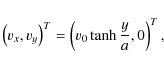
where U0 = 2 v0 is the shear velocity, and a is a length scale characterizing the width of the shear flow. The background density and pressure are uniform, and the thermodynamic properties of the fluid are described by an ideal-gas EOS with an adiabatic index
where
To trigger the KH instability we perturb the shear flow by a
transverse velocity
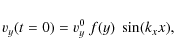
where f (with
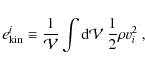
Finally, we introduce the volume-averaged kinetic energy
densities
and volume-averaged magnetic energy densities
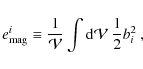
with
4.1 Linear growth
Our code reproduces the growth rate of the KH instability very accurately. To demonstrate this we recalculated some of the models studied by Keppens et al. (1999) (models grw-n in Table A.1). The growth rates for these models are either given in Keppens et al. (1999), or can be obtained from the figures of Miura & Pritchett (1982).
The models have a uniform background density
![]() ,
and a
uniform background pressure P0. We impose open boundary conditions
in the transverse (y) direction, periodic ones in x-direction, and
vary the value of the shear velocity, the width of the shear layer,
and the grid resolution.
,
and a
uniform background pressure P0. We impose open boundary conditions
in the transverse (y) direction, periodic ones in x-direction, and
vary the value of the shear velocity, the width of the shear layer,
and the grid resolution.
We derive growth rates,
![]() ,
from the exponential
growth of
,
from the exponential
growth of
![]() ,
and compare these to the values,
,
and compare these to the values,
![]() ,
given by
Miura & Pritchett (1982) and
Keppens et al. (1999), respectively. We note in this
respect that
,
given by
Miura & Pritchett (1982) and
Keppens et al. (1999), respectively. We note in this
respect that
![]() (see Eq. (10)) grows at twice the rate of
the KH instability. The agreement between the theoretical predictions
and our numerical results is, in general, very good (see
Table A.1 and Fig. 1).
(see Eq. (10)) grows at twice the rate of
the KH instability. The agreement between the theoretical predictions
and our numerical results is, in general, very good (see
Table A.1 and Fig. 1).
After the initial phase of exponential growth, a roughly circular vortex develops in the perturbed non-magnetized shear layer which should be eventually dissipated by (numerical) viscosity. However, this process is very slow for our models (we see no sign of dissipation until the end of our simulations), as the numerical viscosity of our code is very low.
The formation of a single KH vortex rather than of a multitude
of small vortices is not an artifact of the form of the initial
perturbation (Eq. (9)). To demonstrate this, we
simulated a non-magnetic model with random rather than sinusoidal
perturbations of the transverse velocity with an amplitude of
10-6 of the shear velocity (see Fig. 2
for two snapshots of the model simulated with 10242 zones at t =
16 and t = 25.5 (panels (a) and (b), respectively). Initially,
three small KH vortices develop (panel (a)), but after two subsequent
mergers of these vortices, only one large vortex remains (panel (b)),
resembling closely the flow field of a model with sinusoidal
perturbation. Due to this evolution towards a single large-scale
vortex, we focus on models with sinusoidal perturbations in the
following![]() .
.
4.2 Non-magnetic models
We simulated a set of non-magnetic models (summarized in
Table A.2) to study the influence of the box size and
boundary conditions on the evolution of transonic and supersonic
(
![]() )
shear flows. As noted by
Miura & Pritchett (1982), there is no
growing mode for a
)
shear flows. As noted by
Miura & Pritchett (1982), there is no
growing mode for a
![]() shear flow, but in models with closed
boundaries we find nevertheless a growing instability whose growth
mechanism is, however, different (see below).
shear flow, but in models with closed
boundaries we find nevertheless a growing instability whose growth
mechanism is, however, different (see below).
We first consider models with
![]() .
For these models the
instability grows faster when the vertical domain size is enlarged,
and open boundaries yield larger growth rates than reflecting ones.
The reason for this behavior is that the instability affects a larger
region of the flow than in the case of slow shear flows. To
demonstrate this we compare models HD2o-1 and HD2o-1-s that differ
only in the size of the computational domain in y-direction:
.
For these models the
instability grows faster when the vertical domain size is enlarged,
and open boundaries yield larger growth rates than reflecting ones.
The reason for this behavior is that the instability affects a larger
region of the flow than in the case of slow shear flows. To
demonstrate this we compare models HD2o-1 and HD2o-1-s that differ
only in the size of the computational domain in y-direction:
![]() and
and
![]() for models HD2o-1 and HD2o-1-s,
respectively. According to Fig. 3 the
volume-averaged kinetic energy density,
for models HD2o-1 and HD2o-1-s,
respectively. According to Fig. 3 the
volume-averaged kinetic energy density,
![]() ,
grows
faster and leads to much larger values in model HD2o-1 than in model
HD2o-1-s. Furthermore, in model HD2o-1-s the growth of
,
grows
faster and leads to much larger values in model HD2o-1 than in model
HD2o-1-s. Furthermore, in model HD2o-1-s the growth of
![]() shows superimposed oscillations. In both models
waves are created at the shear layer which travel outwards in
y-direction carrying (transverse) kinetic energy. If the waves are
allowed to travel over a sufficiently long distance
shows superimposed oscillations. In both models
waves are created at the shear layer which travel outwards in
y-direction carrying (transverse) kinetic energy. If the waves are
allowed to travel over a sufficiently long distance ![]() (which
is the case for model HD2o-1), they steepen into shock waves when the
fluid velocity exceeds the sound speed. The shocks propagate mainly
in x-direction, advected by the shear flow. Kinetic energy is
dissipated into internal one in these shocks, and the flow develops a
vortex-like structure. If the boundaries of the computational domain
are too close to the shear layer, the waves leave the domain before
they can affect the flow, i.e., the growth rate is reduced. Each time
a wave leaves the computational domain, it carries away kinetic energy
giving rise to the oscillations of
(which
is the case for model HD2o-1), they steepen into shock waves when the
fluid velocity exceeds the sound speed. The shocks propagate mainly
in x-direction, advected by the shear flow. Kinetic energy is
dissipated into internal one in these shocks, and the flow develops a
vortex-like structure. If the boundaries of the computational domain
are too close to the shear layer, the waves leave the domain before
they can affect the flow, i.e., the growth rate is reduced. Each time
a wave leaves the computational domain, it carries away kinetic energy
giving rise to the oscillations of
![]() visible in
Fig. 3.
visible in
Fig. 3.
For an intermediate domain size of
![]() (model
HD2o-1-s), we find despite the absence of oscillations a smaller
growth rate than for models HD2o-1 (
(model
HD2o-1-s), we find despite the absence of oscillations a smaller
growth rate than for models HD2o-1 (
![]() )
and HD2o-1-1 (
)
and HD2o-1-1 (
![]() ), respectively. The boundaries are sufficiently close to
the shear layer to affect the growth of the instability. Saturation
occurs by the same mechanism as in case of a larger domain, namely by
the development of shock waves.
), respectively. The boundaries are sufficiently close to
the shear layer to affect the growth of the instability. Saturation
occurs by the same mechanism as in case of a larger domain, namely by
the development of shock waves.
The distance the waves travel in transverse direction increases with
increasing Mach number of the shear flow. For
![]() the waves
are contained essentially in the region
the waves
are contained essentially in the region
![]() (a
version of model grw-3 simulated on a smaller grid of
(a
version of model grw-3 simulated on a smaller grid of
![]() zones covering a domain of
zones covering a domain of
![]() does not
show oscillation of
does not
show oscillation of
![]() ). For the same reason the
evolution does not depend on whether one imposes reflecting or open
boundary conditions (compare models HD2r-0 in
Table A.2 and grw-3 in
Table A.1). Thus, to encounter a rapidly
growing instability in a fast shear flow, one has to simulate a
sufficiently large domain, or alternatively to use reflecting
boundaries in y-direction. For
). For the same reason the
evolution does not depend on whether one imposes reflecting or open
boundary conditions (compare models HD2r-0 in
Table A.2 and grw-3 in
Table A.1). Thus, to encounter a rapidly
growing instability in a fast shear flow, one has to simulate a
sufficiently large domain, or alternatively to use reflecting
boundaries in y-direction. For
![]() ,
open and closed
models (i.e., models where open or reflecting boundaries are imposed)
agree in their growth rates if simulated on a sufficiently large
domain. However, when the extent of the computational domain is small
in the transverse direction (ly = 0.5), we observe a
destabilization of closed models: the growth rate of the closed model
HD2r-1-s exceeds that of the corresponding open model HD2o-1-s by a
factor of
,
open and closed
models (i.e., models where open or reflecting boundaries are imposed)
agree in their growth rates if simulated on a sufficiently large
domain. However, when the extent of the computational domain is small
in the transverse direction (ly = 0.5), we observe a
destabilization of closed models: the growth rate of the closed model
HD2r-1-s exceeds that of the corresponding open model HD2o-1-s by a
factor of ![]() 3.5. Furthermore, closed models exhibit a phase
of exponential and oscillatory growth of
3.5. Furthermore, closed models exhibit a phase
of exponential and oscillatory growth of
![]() even
when
even
when
![]() ,
whereas open models are stable.
,
whereas open models are stable.
In the KH saturated state the flow consists of a dominant vortex for shear flows of moderate Mach numbers. At large Mach numbers and when the growth of the instability is mediated mainly by shock waves, the flow is characterized by a rather thin and clearly delimited transition layer oriented along the initial discontinuity (at y=0). This layer is surrounded by two regions of anti-parallel flows.
The shocks created at the supersonic shear layer are initially oblique, but eventually become planar shocks parallel to the y-direction. This process happens earlier close to y = 0. The vertical extent of the planar shock structures varies from a fraction of the vertical domain size to almost the whole computational box. When the propagation of the shocks is restricted in y-direction, the fluid tries to avoid these by sliding along the vertical direction. Thus, the planar shocks very efficiently convert x- into y-kinetic energy.
4.3 Intermediate and weak fields
Sufficiently strong magnetic fields (Alfvén number
![]() ;
see Eq. (1)) stabilize the flow according to linear
stability analysis. We indeed observe this stabilization in
simulations of both subsonic and supersonic strongly magnetized shear
flows. In the following, we thus focus on the more interesting case
of intermediate and weak initial fields, which according to
Frank et al. (1996) can give rise to
disruptive and dissipative dynamics, respectively. The
models we describe in this section were computed using a grid with
;
see Eq. (1)) stabilize the flow according to linear
stability analysis. We indeed observe this stabilization in
simulations of both subsonic and supersonic strongly magnetized shear
flows. In the following, we thus focus on the more interesting case
of intermediate and weak initial fields, which according to
Frank et al. (1996) can give rise to
disruptive and dissipative dynamics, respectively. The
models we describe in this section were computed using a grid with
![]() and reflecting boundary conditions in
y-direction. We simulated shear flows with U0 = 1, and varied
the Mach number of the flow by setting the pressure either to P0 =
0.6 or
P0 = 0.0375 corresponding to Mach numbers of
and reflecting boundary conditions in
y-direction. We simulated shear flows with U0 = 1, and varied
the Mach number of the flow by setting the pressure either to P0 =
0.6 or
P0 = 0.0375 corresponding to Mach numbers of
![]() and
and
![]() ,
respectively. The adiabatic index of the gas was
,
respectively. The adiabatic index of the gas was
![]() .
.
4.3.1 Intermediate fields
For
![]() ,
we find, in agreement with
Frank et al. (1996), non-linear stabilization.
The magnetic field is amplified during the linear phase, and the
magnetic tension becomes eventually sufficiently strong to prevent
further bending of the field lines. Thus, the formation of a KH
vortex is suppressed. Instead, the velocityand the magnetic fields
remain essentially aligned with each other and the shear layer
developing only small y-components. After the end of linear growth
a broad shear layer develops inside which the magnetic field has a
sheet-like structure.
,
we find, in agreement with
Frank et al. (1996), non-linear stabilization.
The magnetic field is amplified during the linear phase, and the
magnetic tension becomes eventually sufficiently strong to prevent
further bending of the field lines. Thus, the formation of a KH
vortex is suppressed. Instead, the velocityand the magnetic fields
remain essentially aligned with each other and the shear layer
developing only small y-components. After the end of linear growth
a broad shear layer develops inside which the magnetic field has a
sheet-like structure.
If the magnetic field strength is reduced further (
![]() ), we
observe a linear growth of the KH instability, and the formation of a
KH vortex. The overturning vortex continues to amplify the field
until it becomes eventually so strong that it resists further bending,
i.e. the instability saturates in the non-linear phase. The magnetic
energy, which grows exponentially during the linear phase, reaches a
maximum, and then gradually declines back to almost its initial value.
), we
observe a linear growth of the KH instability, and the formation of a
KH vortex. The overturning vortex continues to amplify the field
until it becomes eventually so strong that it resists further bending,
i.e. the instability saturates in the non-linear phase. The magnetic
energy, which grows exponentially during the linear phase, reaches a
maximum, and then gradually declines back to almost its initial value.
It is important to note that although we are evolving the equations of
ideal (i.e., non-resistive) MHD numerical resistivity is present and
acts similar as a physical resistivity. Hence, reconnection of field
lines and dissipation of magnetic energy into internal energy occurs.
Though being a purely numerical effect, this dissipation mimics a
physical process: in ideal MHD (or for exceedingly large magnetic
Reynolds number
![]() ), energy is transferred to ever
smaller length scales by a turbulent cascade. When the cascade reaches
the scale set by the grid resolution, the physics is no longer
appropriately represented by the discretized magnetic field. Instead,
the unresolved (sub-grid) magnetic energy is assigned to the internal
energy. Hence, numerical resistivity (like numerical viscosity) acts
as an unspecific sub-grid model for unresolved dynamics.
), energy is transferred to ever
smaller length scales by a turbulent cascade. When the cascade reaches
the scale set by the grid resolution, the physics is no longer
appropriately represented by the discretized magnetic field. Instead,
the unresolved (sub-grid) magnetic energy is assigned to the internal
energy. Hence, numerical resistivity (like numerical viscosity) acts
as an unspecific sub-grid model for unresolved dynamics.
As a result of numerical resistivity, our models show the dynamics discussed by Jones et al. (1997): the emergence of coherent flow and field structures, and their subsequent disruption in intense reconnection events whereby kinetic energy is efficiently converted into internal energy. As a consequence, the kinetic energy decreases more strongly than in the non-magnetic case, and the flow barely resembles a KH vortex at the end of the simulation. Instead, we find a broad transition layer that is embedded into two anti-parallel flows and that contains thin magnetic flux sheets. The flow is rather laminar than turbulent, with elongated streaks of gas and field stretching across the computational domain.
4.3.2 Weak fields
Overview:
Models with a weak initial magnetic field show disruptive or dissipative dynamics (Jones et al. 1997). In both regimes, a KH vortex develops. The magnetic field forms thin flux sheets while it is wound up by the vortex. If two flux sheets of opposite polarity come to lie close to each other, they suffer the resistive tearing-mode instability which leads to the reconnection of field lines of different orientation and the conversion of magnetic into thermal energy. Since the magnetic energy was previously amplified at the cost of the kinetic energy, the tearing modes act essentially as a catalyst facilitating the dissipation of kinetic into internal energy. This behavior characterizes the dissipation regime, while in the disruption regime another effect comes into play: the magnetic field eventually becomes sufficiently strong to disrupt the vortex leaving behind a broad transition layer where turbulent flow and magnetic fields decay slowly. The dynamics of the flow and the magnetic field are highly coupled since the field is dominated by flux sheets where the velocity and the magnetic field are strongly aligned, reminiscent of the Alfvén effect in MHD turbulence (Kraichnan 1965; Iroshnikov 1964). Accordingly, we also find near equipartition between the transverse magnetic and kinetic energy densities (see the disruption models below).
The evolution of the simulated weak-field models (summarized in Table A.3) consists of three distinct phases:
- Linear KH growth phase: initial perturbations of both velocity and magnetic field grow exponentially until a KH vortex forms.
- Kinematic field amplification phase: magnetic field is wound up by the secularly evolving KH vortex.
- Dissipation/disruption phase: KH vortex looses its energy due to magnetic stresses and resistive effects.
![\begin{figure}
\par\includegraphics[width=7.4cm,clip]{13386F05a} \vspace*{3.5mm}
\end{figure}](/articles/aa/full_html/2010/07/aa13386-09/img114.png)
|
Figure 5:
Growth of the volume-averaged turbulent (transverse)
magnetic energy density
|
KH growth phase:
Early on during the evolution the seed perturbations imposed on the initial shearing profile are amplified exponentially, but the magnetic field remains too weak to affect the evolution. When the exponential growth of the KH instability terminates, the total magnetic energy has grown by about a factor 1.4 in all models, the contribution of the transverse field component by amounting to about 10%. Due to the persisting weakness of the magnetic field the growth rate of the instability and the flow structure after the end of the KH growth phase are the same as those without any field.
When the KH instability saturates with the formation of a KH vortex
(see Fig. 6 for a model with
![]() ), the growth of the transverse kinetic energy ceases, too
(Fig. 4). Density, pressure, sound speed, and
magnetic field strength possess a minimum at the center of the vortex,
and the magnetic field is wound up into a long thin sheet surrounding
the vortex. These findings hold for the models with
), the growth of the transverse kinetic energy ceases, too
(Fig. 4). Density, pressure, sound speed, and
magnetic field strength possess a minimum at the center of the vortex,
and the magnetic field is wound up into a long thin sheet surrounding
the vortex. These findings hold for the models with
![]() and
and
![]() ,
respectively. Fig. 5 shows that the
growth rate of the instability (the slope of the curves) is
independent of the grid resolution and the initial field strength for
,
respectively. Fig. 5 shows that the
growth rate of the instability (the slope of the curves) is
independent of the grid resolution and the initial field strength for
![]() .
.
Kinematic amplification phase:
After saturation of the essentially hydrodynamic KH instability,
![]() exhibits small oscillations about a
constant value. The initial shearing interface, wound up several
times by the overturning vortex, has become a thin fluid layer
separating flow regions of opposite velocities
Fig. 6). The magnetic sheet is being
stretched by the overturning vortex giving rise to an exponential
amplification of the field (instead of a linear one by winding), as
the growth rate due to stretching depends on the field strength
itself. In spite of the growing magnetic field the flow structure as
well as the kinetic and internal energies of the fluid show only minor
changes throughout the entire kinematic amplification phase.
exhibits small oscillations about a
constant value. The initial shearing interface, wound up several
times by the overturning vortex, has become a thin fluid layer
separating flow regions of opposite velocities
Fig. 6). The magnetic sheet is being
stretched by the overturning vortex giving rise to an exponential
amplification of the field (instead of a linear one by winding), as
the growth rate due to stretching depends on the field strength
itself. In spite of the growing magnetic field the flow structure as
well as the kinetic and internal energies of the fluid show only minor
changes throughout the entire kinematic amplification phase.
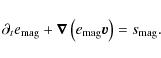
To understand the amplification of the magnetic field in detail we
consider the sources and sinks of magnetic energy. From the scalar
product of
![]() (given by the induction equation) and
the magnetic field,
(given by the induction equation) and
the magnetic field,
![]() ,
one can derive
the equation for the evolution of the total energy density of the
magnetic field,
,
one can derive
the equation for the evolution of the total energy density of the
magnetic field,
![]() ,
which has the form of an advection
equation with source terms,
,
which has the form of an advection
equation with source terms,
The source term,
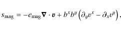
consists of a compression term proportional to the divergence of the velocity field, and a shear term proportional to the curl of the velocity field. The sum of both terms (i.e., the source term) is negative, when the magnetic field does work on the fluid.
The evolution of
![]() is exemplified in
Fig. 7 for a model with
is exemplified in
Fig. 7 for a model with
![]() .
As the fluid is nearly incompressible in our models, the first
term on the r.h.s. of Eq. (13) is small, and field
amplification (bluish areas) occurs predominantly by stretching. As
there is no back-reaction onto the flow, the volume-averaged
transverse magnetic energy density grows exponentially with
time. Stretching mainly happens in the thin flux sheet passing through
the origin of the grid, and to a lesser extent in the flux sheets
located closer to the center of the vortex. There even a small
reduction of
.
As the fluid is nearly incompressible in our models, the first
term on the r.h.s. of Eq. (13) is small, and field
amplification (bluish areas) occurs predominantly by stretching. As
there is no back-reaction onto the flow, the volume-averaged
transverse magnetic energy density grows exponentially with
time. Stretching mainly happens in the thin flux sheet passing through
the origin of the grid, and to a lesser extent in the flux sheets
located closer to the center of the vortex. There even a small
reduction of
![]() can be observed (see
Fig. 7). The volume integral of the
source term over the entire computational domain is positive, i.e.,
the magnetic energy of the models is increasing.
can be observed (see
Fig. 7). The volume integral of the
source term over the entire computational domain is positive, i.e.,
the magnetic energy of the models is increasing.
Because field amplification is mediated by a well resolved, rather
smooth flow, the growth rate of the turbulent magnetic energy density
![]() is independent of the grid resolution during the
kinematic amplification phase (
is independent of the grid resolution during the
kinematic amplification phase (
![]() ;
see
Fig. 5). Models with
;
see
Fig. 5). Models with
![]() ,
but otherwise
identical initial conditions and grid resolution, show a slower growth
of the field (see Table A.3). As
,
but otherwise
identical initial conditions and grid resolution, show a slower growth
of the field (see Table A.3). As
![]() (monitoring the turnover velocity of the vortex)
shows small variations with time during the kinematic amplification
phase (see Fig. 4), the growth rate varies
slightly, too (note the variation of the slope in
Fig. 5 for
(monitoring the turnover velocity of the vortex)
shows small variations with time during the kinematic amplification
phase (see Fig. 4), the growth rate varies
slightly, too (note the variation of the slope in
Fig. 5 for
![]() ).
).
The evolution of the turbulent magnetic energy density after the end
of the kinematic amplification phase depends strongly on the grid
resolution and the initial field strength (Fig. 5).
Comparing the results for the models with
![]() and
and
![]() we conclude that the growth of the turbulent magnetic energy
density is less for models with a stronger initial field than for
those with a weaker initial field at the same grid resolution.
we conclude that the growth of the turbulent magnetic energy
density is less for models with a stronger initial field than for
those with a weaker initial field at the same grid resolution.
For the model with
![]() the magnetic field eventually reaches
locally (within a factor of a few) equipartition strength, i.e.,
magnetic stresses start to change the flow. In the model with the
lower initial Alfvén velocity (i.e., larger Alfvén number), the
magnetic field remains, in spite of a larger amplification, too weak
to cause such an effect.
the magnetic field eventually reaches
locally (within a factor of a few) equipartition strength, i.e.,
magnetic stresses start to change the flow. In the model with the
lower initial Alfvén velocity (i.e., larger Alfvén number), the
magnetic field remains, in spite of a larger amplification, too weak
to cause such an effect.
![\begin{figure}
\par\includegraphics[width=7.2cm,clip]{13386F07a}
\end{figure}](/articles/aa/full_html/2010/07/aa13386-09/img126.png)
|
Figure 7: Snapshot of the source term of the total magnetic energy density (Eq. (13)) for the model shown in Fig. 6 taken during the kinematic amplification phase. Reddish (bluish) colors show regions where the total magnetic energy density increases (decreases). |
To quantify the amount of amplification of the magnetic field occurring
during the kinematic amplification phase we introduce the field
amplification factor
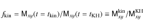
defined as the ratio of the off-diagonal volume-integrated Maxwell stress component
When plotting
![]() as a function of grid resolution and
initial Alfvén number we find that our models populate the lower
right region (shaded in gray) in both diagrams
(Fig. 8). Both for a given grid
resolution and initial Alfvén number,
as a function of grid resolution and
initial Alfvén number we find that our models populate the lower
right region (shaded in gray) in both diagrams
(Fig. 8). Both for a given grid
resolution and initial Alfvén number,
![]() converges
towards a maximum value with increasing initial Alfvén number
(Fig. 8, left panel), and increasing grid
resolution (Fig. 8, right panel). This
convergence is also obvious from the graph of
converges
towards a maximum value with increasing initial Alfvén number
(Fig. 8, left panel), and increasing grid
resolution (Fig. 8, right panel). This
convergence is also obvious from the graph of
![]() for
for
![]() (Fig. 8, left
panel); note that for large values of
(Fig. 8, left
panel); note that for large values of
![]() even our finest the grid
spacing was not yet sufficient to show the flattening of
even our finest the grid
spacing was not yet sufficient to show the flattening of
![]() .
.
The panels further show that the weaker (larger) the initial field
(the value of
![]() ), the higher is the amplification factor
), the higher is the amplification factor
![]() achievable during the kinematic amplification phase.
The upper border of the gray shaded regions is approximately given by
the power laws mx7/8 and
achievable during the kinematic amplification phase.
The upper border of the gray shaded regions is approximately given by
the power laws mx7/8 and
![]() ,
respectively.
,
respectively.
![\begin{figure}
\par\includegraphics[width=12cm,clip]{13386F08a}\vspace*{3.4mm}
\end{figure}](/articles/aa/full_html/2010/07/aa13386-09/img134.png)
|
Figure 8:
Amplification of the magnetic field during the kinematic amplification phase: the amplification factor,
|
To explain these results and to quantify the effects of the grid
resolution, we define a characteristic length scale of variations of
the magnetic field

where the denominator is proportional to the current density. Initially infinite (the initial magnetic field is curl free), lbdecreases during the KH growth and the kinematic amplification phases.
Due to flux conservation, the amplification of the field occurring
mainly in flux sheets goes along with a decrease of the width of the
sheets orthogonal to the magnetic field, which is roughly given by
lb. In simulations, the decrease of lb can properly be
followed only as long as
![]() ,
where
,
where
![]() is the
finite grid spacing. When this limit is reached the exponential
amplification of the field strength and field energy ceases. Further
growth only regards the magnetic energy, which can increase at most
linearly with time due to the increasing length of the sheet (at a
constant width!). This point in the evolution marks the end of the
phase of kinematic amplification.
is the
finite grid spacing. When this limit is reached the exponential
amplification of the field strength and field energy ceases. Further
growth only regards the magnetic energy, which can increase at most
linearly with time due to the increasing length of the sheet (at a
constant width!). This point in the evolution marks the end of the
phase of kinematic amplification.
Consequently, there exists an upper limit for the amplification of the
magnetic field strength attainable by flux-sheet stretching that
depends on the grid resolution. However, this limit set by the ratio
of the grid spacing and the initial thickness of the flux sheet can
only be reached, if the field strength remains dynamically negligible
(i.e. below equipartition strength) during the kinematic amplification
phase. This applies to models with weak initial magnetic fields
(
![]() ), which are located near the upper border of the
gray shaded region in the left panel of
Fig. 8.
), which are located near the upper border of the
gray shaded region in the left panel of
Fig. 8.
If the magnetic field reaches - within a factor of order unity -
local equipartition strength during the kinematic amplification phase,
the flow dynamics and as a consequence the termination of that phase
show distinct features. This is the case for models with strong
initial magnetic fields (
![]() )
and sufficiently fine
resolution, which are located near the upper border of the gray shaded
region in the right panel of Fig. 8. For
these models
)
and sufficiently fine
resolution, which are located near the upper border of the gray shaded
region in the right panel of Fig. 8. For
these models
![]() ,
i.e., the amplification
is larger for weaker initial fields. One factor contributing to this
trend is the back-reaction of the field onto the flow. When locally
the Alfvén number approaches the order of unity (see, e.g., the
lower panel of Fig. 9), magnetic
stresses start to decelerate the fluid in the flux sheets, and as the
flux sheets partially thread the KH vortex its rotational velocity
decreases, too. Consequently, the amplification factor will be smaller
in this case than for an initially less strongly magnetized model.
Finally, note that for models with weak initial magnetic fields
(
,
i.e., the amplification
is larger for weaker initial fields. One factor contributing to this
trend is the back-reaction of the field onto the flow. When locally
the Alfvén number approaches the order of unity (see, e.g., the
lower panel of Fig. 9), magnetic
stresses start to decelerate the fluid in the flux sheets, and as the
flux sheets partially thread the KH vortex its rotational velocity
decreases, too. Consequently, the amplification factor will be smaller
in this case than for an initially less strongly magnetized model.
Finally, note that for models with weak initial magnetic fields
(
![]() )
we do not observe effects due to back-reaction, as
this requires larger field amplification factors than reached in our
simulations due to insufficient grid resolution (see discussion above).
)
we do not observe effects due to back-reaction, as
this requires larger field amplification factors than reached in our
simulations due to insufficient grid resolution (see discussion above).
A second important issue for understanding our results is the effect
of numerical resistivity. Although we integrate the equations of
ideal MHD, the numerical scheme employed in our code mimics to
some degree the effects of physical resistivity due to its
inherent numerical resistivity. Thus, the numerical scheme
smooths sharp features in the magnetic field and causes violent
resistive instabilities of, e.g., tearing-mode type. The latter effect
is most pronounced at length scales close to the grid spacing
![]() .
.
When the typical length scales of the magnetic field - given
approximately by lb - are comparable to the grid spacing
![]() ,
we expect numerical resistivity to be important. For the
model with
,
we expect numerical resistivity to be important. For the
model with
![]() ,
,
![]() ,
and
mx = 2048 zones
,
and
mx = 2048 zones
![]() inside the flux sheet near the end of the kinematic
amplification phase (Fig. 9, upper
panel). The magnetic field is dominated by a complex pattern of
sheets partially arranged in pairs or even triplets with anti-parallel
fields. An example is the triple sheet structure passing roughly
diagonally through the origin from down left to top right
(Fig. 9, upper panel). This triplet
consisting of a central sheet with bx > 0 and two parallel ``wing''
sheets with bx < 0 is the result of the advection of magnetic flux
towards the central sheet by the flow.
inside the flux sheet near the end of the kinematic
amplification phase (Fig. 9, upper
panel). The magnetic field is dominated by a complex pattern of
sheets partially arranged in pairs or even triplets with anti-parallel
fields. An example is the triple sheet structure passing roughly
diagonally through the origin from down left to top right
(Fig. 9, upper panel). This triplet
consisting of a central sheet with bx > 0 and two parallel ``wing''
sheets with bx < 0 is the result of the advection of magnetic flux
towards the central sheet by the flow.
As the advection continues the strength of the magnetic field in the
side sheets increases, while their width decreases leading to intense
currents. Eventually
![]() ,
and resistive instabilities
(tearing modes) start to grow, which curl up the two wing sheets and
eventually disrupt them leaving behind only the central sheet
(Fig. 9, upper panel). This process
affects the entire triple sheet structure
(Fig. 9, lower panel).
,
and resistive instabilities
(tearing modes) start to grow, which curl up the two wing sheets and
eventually disrupt them leaving behind only the central sheet
(Fig. 9, upper panel). This process
affects the entire triple sheet structure
(Fig. 9, lower panel).
Shortly afterwards, the central sheet of the former triplet, still intact, is disrupted. From the interior of the vortex further sheets of magnetic flux are expelled creating new strong currents that again suffer strong resistive instabilities. This cycle of processes repeats every time strong currents build up by approaching flux sheets. As a consequence, the large coherent flux sheet structures are disrupted, and reconnection of magnetic field lines leads to numerous small-scale field structures including closed field loops, similarly to those reported in previous simulations (e.g., Keppens et al. 1999).
The amplification of the magnetic field terminates due to the development of these resistive instabilities, because (i) they convert magnetic energy into thermal energy; and because (ii) the resulting small-scale field and flow is less efficient in amplifying the magnetic field than a more coherent flow.
The mechanism just described is responsible for the termination of the
kinematic amplification phase in well resolved models. All models
with
![]() ,
mx > 256 and
,
mx > 256 and
![]() ,
mx > 1024 undergo
this evolution. For even finer grids the results are essentially
converged in terms of the amplification factor
,
mx > 1024 undergo
this evolution. For even finer grids the results are essentially
converged in terms of the amplification factor
![]() (Fig. 8). Finding convergence for a flow
whose behavior depends strongly on numerical resistivity is a
remarkable result that deserves some explanation. Naturally, one would
expect that with finer grid resolution (i.e., decreasing numerical
resistivity) tearing modes are better suppressed, thus enabling the
field to grow stronger.
(Fig. 8). Finding convergence for a flow
whose behavior depends strongly on numerical resistivity is a
remarkable result that deserves some explanation. Naturally, one would
expect that with finer grid resolution (i.e., decreasing numerical
resistivity) tearing modes are better suppressed, thus enabling the
field to grow stronger.
However, this reasoning does only apply, if the main effect of
numerical resistivity is the disruption of isolated flux sheets. In
such a situation, the magnetic field in the flux sheet will be
amplified until tearing modes grow faster than the field strength
increases. As soon as the stretching of the flux sheet leads to a
combination of a sufficiently strong field and a sufficiently thin
sheet (both conditions as well as an increasing resistivity imply
higher growth rates of resistive instabilities; see e.g.,
Biskamp 2000) tearing modes would start
to disrupt the sheet. The amount of stretching necessary to reach
this state depends on the resistivity, i.e., in our case on the grid
resolution: finer grids require stronger fields and thinner sheets for
disruption. Hence, the maximum field strength achievable at disruption
should grow with increasing grid resolution, but the situation in our
models described above is crucially different. Instead of operating on
an isolated current sheet in a static background, the resistive
instabilities terminating the growth of the magnetic energy act in our
models on a multitude of flux sheets approaching each other closely
due to a dynamic background flow. Their growth rates can become
faster than the kinematic amplification of the field once the
distance, ![]() ,
between two sheets rather than the width of
the sheets, lb, becomes sufficiently small, i.e,
,
between two sheets rather than the width of
the sheets, lb, becomes sufficiently small, i.e,
![]() ,
but
,
but
![]() .
Contrary to the sheet width lb, the distance
.
Contrary to the sheet width lb, the distance ![]() is not related to the magnetic energy stored in the
sheets, but it is determined mainly by the flow field. Hence, there
exists a relation between the velocity field and the instance of
growth termination. The velocity field, in turn, depends mainly on
the hydrodynamics of the KH vortex, and only weakly on the grid
resolution, i.e., the moment when the flux sheets break up is
independent of resolution. The latter also holds for the energy
contained in the sheets. Converged results for the amplification
factor can therefore be obtained despite the presence of a grid
spacing dependent numerical resistivity.
is not related to the magnetic energy stored in the
sheets, but it is determined mainly by the flow field. Hence, there
exists a relation between the velocity field and the instance of
growth termination. The velocity field, in turn, depends mainly on
the hydrodynamics of the KH vortex, and only weakly on the grid
resolution, i.e., the moment when the flux sheets break up is
independent of resolution. The latter also holds for the energy
contained in the sheets. Converged results for the amplification
factor can therefore be obtained despite the presence of a grid
spacing dependent numerical resistivity.
As we saw above, the tearing modes of our models are triggered first
after the formation of multiple sheet structures. At this point the
central flux sheet of the triplet passing through the origin is still
well resolved by several zones (
![]() ), but the distance
), but the distance ![]() between the side sheets and the
central sheet approaches
between the side sheets and the
central sheet approaches
![]() as the former are advected towards
the latter one.
as the former are advected towards
the latter one.
Some of our model sequences show no convergence behavior
(Fig. 8, left panel), as the grid
resolution necessary for that increases with the initial Alfvén
number. For very weak initial fields (
![]() )
even our finest
grid with 40962 zones does not yield a resolution-independent
amplification factor. However, as the advection of the flux sheets
does not depend on resolution and only weakly on the strength of the
initial field (except for the sheets feedback is very limited in the
kinematic amplification phase), the formation of unstable multiple
sheets is possible even on coarse grids. Nevertheless, we do not
observe strong resistive instabilities during this phase for these
models.
)
even our finest
grid with 40962 zones does not yield a resolution-independent
amplification factor. However, as the advection of the flux sheets
does not depend on resolution and only weakly on the strength of the
initial field (except for the sheets feedback is very limited in the
kinematic amplification phase), the formation of unstable multiple
sheets is possible even on coarse grids. Nevertheless, we do not
observe strong resistive instabilities during this phase for these
models.
We showed above that the growth rate of resistive instabilities during
the kinematic amplification phase depends, apart from the resistivity,
on the width of the flux sheet and the field strength, and that this
phase ends when the tearing modes grow faster than the field is
kinematically amplified by the velocity field. To match this
condition, sufficiently strong fields are required during close
encounters of flux sheets. This fact explains why we do not find
resistive instabilities in models with too weak initial fields or too
coarse resolution. In these cases the limitation of the maximum field
strength of a flux sheet imposed by its minimum (resolvable) width
leads to a reduced growth rate of resistive instabilities even when
![]() ,
i.e., the distance between two flux sheets is
reduced to the grid spacing. Thus, these instabilities cannot
terminate the kinematic field amplification process the same way as
they do it in the case of stronger initial fields or finer grids.
,
i.e., the distance between two flux sheets is
reduced to the grid spacing. Thus, these instabilities cannot
terminate the kinematic field amplification process the same way as
they do it in the case of stronger initial fields or finer grids.
The field strength required for resistive instabilities to terminate the kinematic amplification phase depends on the flow field: faster shear flows require stronger fields. Empirically, we find that the maximum field strength at termination corresponds roughly to an Alfvén number of order unity, i.e., to field strengths similar to those required for dynamic feedback.
To summarize, we find that there exist two different mechanisms to terminate the kinematic amplification phase.
- Passive termination: the magnetic field strength reaches
a maximum when the decreasing thickness of the flux sheets
approaches the grid spacing, i.e., when
 .
.
- Resisto-dynamic termination: the magnetic field reaches equipartition strength with the flow field when a combination of dynamic and resistive processes terminate further field growth. Lorentz forces reduce the rotational velocity of the KH vortex, while resistive instabilities develop as flux sheets merge.
Total amplification:
The total amplification of the magnetic field is given by its growth during both the KH and the kinematic amplification phases.
According to our results the field amplification factor
![]() (Eq. (14)) scales with the initial Alfvén
number,
(Eq. (14)) scales with the initial Alfvén
number,
![]() ,
approximately as
,
approximately as
![]() (see
Fig. 8). Consequently, the maximum
Maxwell stress obtainable at the end of the kinematic amplification
phase scales with the initial magnetic field
(see
Fig. 8). Consequently, the maximum
Maxwell stress obtainable at the end of the kinematic amplification
phase scales with the initial magnetic field
![]() approximately as
approximately as

since
The total amplification factors for the magnetic energy, fe,
and the magnetic field strength, fb, are listed for various
models in Table A.3 and displayed in
Fig. 10. The trends described above also hold
here. The amplification factors increase with finer grid resolution
and eventually converge, the resolution required for convergence being
higher for weaker fields. The converged amplification factors are
larger for weaker magnetic fields, scaling as
![]() and
and
![]() ,
respectively. Note that the
latter scaling implies a maximum field strength that is independent of
the initial field strength, consistent with the fact that there exists
a hydrodynamic limit of the magnetic KH instability for weak fields
(see above).
,
respectively. Note that the
latter scaling implies a maximum field strength that is independent of
the initial field strength, consistent with the fact that there exists
a hydrodynamic limit of the magnetic KH instability for weak fields
(see above).
For models differing by their initial hydrodynamic state (i.e, initial
Mach number
![]() ,
and initial shear layer width a; see
Sect. 4) both amplification factors scale very similarly
with the initial field strength (Fig. 10). In
models with a smaller initial Mach number but the same initial shear
layer width (
,
and initial shear layer width a; see
Sect. 4) both amplification factors scale very similarly
with the initial field strength (Fig. 10). In
models with a smaller initial Mach number but the same initial shear
layer width (
![]() ,
a=0.05; filled green circles), and with
the same initial Mach number but an initially wider shear layer
(
,
a=0.05; filled green circles), and with
the same initial Mach number but an initially wider shear layer
(
![]() ,
a = 0.15; red diamonds) the KH instability grows
slower than in standard model (
,
a = 0.15; red diamonds) the KH instability grows
slower than in standard model (
![]() ,
a=0.05) discussed
above. It also saturates at smaller transverse kinetic energies
(
,
a=0.05) discussed
above. It also saturates at smaller transverse kinetic energies
(![]()
![]() and
and ![]()
![]() ,
respectively, instead of
,
respectively, instead of ![]()
![]() ), which implies
a slower kinematic amplification of the field. Hence, fb is
smaller, but its scaling
), which implies
a slower kinematic amplification of the field. Hence, fb is
smaller, but its scaling
![]() is similar to that of the
reference models. Independent of the properties of the initial shear
flow, we find
is similar to that of the
reference models. Independent of the properties of the initial shear
flow, we find
![]() ,
the proportionality constant
depending, however, in a complex way on the initial state. For fixed
shear layer width, slower shear flows lead to less efficient field
amplification. The amplification factor of the magnetic energy
fe, on the other hand, is practically independent of the shear
layer width, while fb decreases for narrower initial shear
layers. However, since the volume where amplification takes place is
larger than that given by the initial shear layer width, overall the
total magnetic energy grows as in the case of a narrower transition
layer.
,
the proportionality constant
depending, however, in a complex way on the initial state. For fixed
shear layer width, slower shear flows lead to less efficient field
amplification. The amplification factor of the magnetic energy
fe, on the other hand, is practically independent of the shear
layer width, while fb decreases for narrower initial shear
layers. However, since the volume where amplification takes place is
larger than that given by the initial shear layer width, overall the
total magnetic energy grows as in the case of a narrower transition
layer.
To summarize, the maximum magnetic field achieved is mainly a function of the overturning velocity of the KH vortex, corresponding to the transverse kinetic energy, while the magnetic energy at the termination of the growth depends on the initial Mach number, on the width of the shear profile and on the initial magnetic field.
Saturation, dissipation and disruption:
After termination of the amplification of the magnetic field, the shear flow enters the saturation phase. We will discuss in the following mainly models encountering a resisto-dynamic termination rather than a passive one, but also briefly mention the behavior of models suffering a passive termination of the field growth.
As a typical example, we illustrate the evolution of the partial
energies of the model with
![]() and
and
![]() in
Fig. 11. After the end of the kinematic
amplification phases both the kinetic energy
in
Fig. 11. After the end of the kinematic
amplification phases both the kinetic energy
![]() (shear
component) and
(shear
component) and
![]() (transverse component) decrease, while
the internal energy increases. The magnetic energy remains roughly at
the level it has reached at the end of the kinematic amplification
phase. In the final state, the transverse kinetic energy is less than
the total magnetic energy, and equal to the transverse magnetic
energy.
(transverse component) decrease, while
the internal energy increases. The magnetic energy remains roughly at
the level it has reached at the end of the kinematic amplification
phase. In the final state, the transverse kinetic energy is less than
the total magnetic energy, and equal to the transverse magnetic
energy.
To understand these results, we compare the model structure at the
beginning of the saturation phase with that near the end of the
simulation. According to Fig. 12 the model
exhibits clear signs of disruptive dynamics
(see Jones et al. 1997). The KH vortex is
still visible as a coherent pattern at t = 34.4, i.e., shortly after
the end of the kinematic amplification phase (panel a). At t =
81.5 the vortex is disrupted, the flow field is dominated by a broad
transition region separating oppositely directed shear flows, and the
y-component of the velocity shows small-scale structures (see patchy
colors in upper part of Fig. 12, panel b).
The magnetic field is concentrated into a multitude of thin flux
sheets with a typical length scale
![]() .
Due to
magnetic reconnection the sheets possess a complex topology. Several
closed field loops have formed that are stabilized by a combination
magnetic loop tension and total pressure (
.
Due to
magnetic reconnection the sheets possess a complex topology. Several
closed field loops have formed that are stabilized by a combination
magnetic loop tension and total pressure (
![]() ). The
flux sheet pattern is imprinted onto the flow field and the gas
pressure distribution. Although the gas pressure is reduced inside the
sheets there is sufficient magnetic pressure to keep the flux sheets
in pressure equilibrium with their surroundings. That explains why the
distribution of the total pressure is rather featureless.
). The
flux sheet pattern is imprinted onto the flow field and the gas
pressure distribution. Although the gas pressure is reduced inside the
sheets there is sufficient magnetic pressure to keep the flux sheets
in pressure equilibrium with their surroundings. That explains why the
distribution of the total pressure is rather featureless.
As visible in Fig. 9 (panel b) and Fig. 12 (panel a), the resistive instabilities responsible for the termination of the kinematic amplification phase spread along the flux sheets leading to a complex field topology and inhibiting further growth of the field not only locally but in the entire volume.
Locally, i.e. inside the flux sheets, the magnetic field is in
equipartition with the velocity field (globally it is still an order
of magnitude weaker). In resistive instabilities magnetic energy is
converted into internal one. Since the magnetic field has been built
up previously at the expense of the kinetic energy, the instabilities
actually mediate the transformation of kinetic energy into internal
energy, hence acting akin to a hydrodynamic viscosity. Eventually, a
steady state (in a statistical sense) develops where the magnetic
energy, and thus the effective viscosity, becomes time-independent,
while kinetic energy is converted into internal one at a constant
rate. After the disruption of the KH vortex, the transverse velocity
reflects the turbulence resulting from the resistive instabilities,
i.e.,
![]() is a measure (like the magnetic field
strength) of the intensity of turbulence. Consequently,
is a measure (like the magnetic field
strength) of the intensity of turbulence. Consequently,
![]() remains constant at saturation, and the disruption
of the KH vortex can be identified by the instance when
remains constant at saturation, and the disruption
of the KH vortex can be identified by the instance when
![]() .
.
The saturation level of the magnetic field, and thus the effective
viscosity, is set by its level at the termination of the kinematic
amplification phase. This level decreases with decreasing initial
field strength, i.e. the weaker the initial field the slower is the
resistive disruption of the KH vortex. To quantify this effect, we
define a disruption time,
![]() ,
as the time when
,
as the time when
![]() falls below
falls below
![]() ,
and a deceleration
rate
,
and a deceleration
rate
![]()
![]() .
Both quantities are listed in Table A.4, and
.
Both quantities are listed in Table A.4, and
![]() and
and
![]() are also shown as a function
of the initial Alfvén number in Fig. 13. For
models with very weak deceleration, the evolution of the kinetic
energy is dominated by large oscillations. Thus, the determination of
the value of
are also shown as a function
of the initial Alfvén number in Fig. 13. For
models with very weak deceleration, the evolution of the kinetic
energy is dominated by large oscillations. Thus, the determination of
the value of
![]() is uncertain to some degree in
these cases, and the numerical values quoted in
Table A.4 should be taken with care.
is uncertain to some degree in
these cases, and the numerical values quoted in
Table A.4 should be taken with care.
Depending on the initial field strength, the models require a certain
minimum resolution to obtain converged values for
![]() and
and
![]() ,
respectively. If the resolution is too low,
the disruption of the vortex and the deceleration of the shear flow
proceed too slow due to an insufficient amount of field amplification.
In the following, we will focus on converged or nearly converged
models.
,
respectively. If the resolution is too low,
the disruption of the vortex and the deceleration of the shear flow
proceed too slow due to an insufficient amount of field amplification.
In the following, we will focus on converged or nearly converged
models.
The disruption and deceleration time scale with the initial field
strength roughly as
b0-0.7. Comparing these times for models with
different initial shear profiles, we find that the disruption time
depends sensitively on both
![]() and the initial shear layer width a. The larger the amplification factor of the magnetic energy
fe is for a given shear profile (see
Fig. 10), the faster is the disruption of the
vortex. The deceleration time, on the other hand, shows a weaker
dependence on
and the initial shear layer width a. The larger the amplification factor of the magnetic energy
fe is for a given shear profile (see
Fig. 10), the faster is the disruption of the
vortex. The deceleration time, on the other hand, shows a weaker
dependence on
![]() and a. Even for a = 0.2, which implies a
much slower KH growth and a very low saturation level of
and a. Even for a = 0.2, which implies a
much slower KH growth and a very low saturation level of
![]() ,
the deceleration time is very
similar to that of the models discussed above, although the magnetic
field strength is much smaller.
,
the deceleration time is very
similar to that of the models discussed above, although the magnetic
field strength is much smaller.
For weaker fields, whose growth ends due to passive instead of resisto-dynamic termination (i.e., non-converged models), the kinetic energy decreases much more slowly. Resistive instabilities grow much slower in such models, because of the growth of their field strength is restricted by numerical resolution. Hence, the effective viscosity is much lower in these models than in well resolved ones.
4.4 Supersonic shear flows
We simulated supersonic shear flows with a Mach number
![]() using the same velocity profile as for the model with
using the same velocity profile as for the model with
![]() ,
but
a reduced gas pressure of
P = 0.0375. In the following, we compare
models with very large (
,
but
a reduced gas pressure of
P = 0.0375. In the following, we compare
models with very large (
![]() )
and small (
)
and small (
![]() )
Alfvén numbers. For the simulations we used grids with a resolution
between 1282 and 20482 zones. As the main result we find that
the growth rate of the magnetic field is lower in supersonic shear
flows than in sonic and subsonic shear flows.
)
Alfvén numbers. For the simulations we used grids with a resolution
between 1282 and 20482 zones. As the main result we find that
the growth rate of the magnetic field is lower in supersonic shear
flows than in sonic and subsonic shear flows.
For
![]() ,
none of the simulations shows an effect of the
magnetic field on the flow. For all grid resolutions the early
evolution of the magnetic model (shock formation and interaction) is
similar to that of the non-magnetic one. Until
,
none of the simulations shows an effect of the
magnetic field on the flow. For all grid resolutions the early
evolution of the magnetic model (shock formation and interaction) is
similar to that of the non-magnetic one. Until ![]() the
transverse kinetic energy increases roughly exponentially before
leveling off (Fig. 11, panel b). The magnetic
field in y-direction is amplified at a similar rate as the kinetic
energy until
the
transverse kinetic energy increases roughly exponentially before
leveling off (Fig. 11, panel b). The magnetic
field in y-direction is amplified at a similar rate as the kinetic
energy until
![]() ,
when the amplification rate increases
strongly. This phase of efficient field growth, lasting until
,
when the amplification rate increases
strongly. This phase of efficient field growth, lasting until
![]() ,
corresponds to the formation of large regions of
subsonic flow where most of the field amplification occurs. The
magnetic field is concentrated in thin sheets. While dominated by a
multitude of shock waves during early phases, the model shows a
subsonic vortical flow in the final state, similarly to the models
discussed in the previous subsection. The kinetic energy has
decreased by a factor of four during the entire evolution. Most of
this deceleration has occurred during the early saturation phase of
the KH instability when the magnetic field is amplified most strongly.
,
corresponds to the formation of large regions of
subsonic flow where most of the field amplification occurs. The
magnetic field is concentrated in thin sheets. While dominated by a
multitude of shock waves during early phases, the model shows a
subsonic vortical flow in the final state, similarly to the models
discussed in the previous subsection. The kinetic energy has
decreased by a factor of four during the entire evolution. Most of
this deceleration has occurred during the early saturation phase of
the KH instability when the magnetic field is amplified most strongly.
Comparing the evolution of the magnetic energy for simulations with different grid resolution, we find trends similar to those of subsonic models with dynamically negligible fields. Stronger magnetic fields are obtained for finer grids the explanation for this behavior being the same as that for the resisto-dynamic termination for subsonic shear flows: amplification ceases when the width of a flux sheet becomes comparable to the grid spacing.
In models with
![]() and
and
![]() the magnetic field
modifes the dynamics. In early stages, a number of weak shock waves
form. Interacting with magnetic flux sheets close to the shearing
interface, theses shocks are disrupted. Spreading away from the
interface in positive and negative y-direction, a wide region of
subsonic flow forms. Both its geometry and formation differ from
those of subsonic shear flows. In barely magnetized models, a subsonic
flow possessing a considerable transversal extent results from the
interaction of oblique shocks (see Sect. 4.2), whereas in
more strongly magnetized models the magnetic field enforces a
subsonic region elongated along the x-direction. We find
convergence with respect to the saturation level of the magnetic
energy, whose value is in general below the value of subsonic models.
At late times, we observe equipartition between the transverse kinetic
energy and the magnetic energy. The deceleration times of the flow
are fairly similar to those of the non-magnetic models.
the magnetic field
modifes the dynamics. In early stages, a number of weak shock waves
form. Interacting with magnetic flux sheets close to the shearing
interface, theses shocks are disrupted. Spreading away from the
interface in positive and negative y-direction, a wide region of
subsonic flow forms. Both its geometry and formation differ from
those of subsonic shear flows. In barely magnetized models, a subsonic
flow possessing a considerable transversal extent results from the
interaction of oblique shocks (see Sect. 4.2), whereas in
more strongly magnetized models the magnetic field enforces a
subsonic region elongated along the x-direction. We find
convergence with respect to the saturation level of the magnetic
energy, whose value is in general below the value of subsonic models.
At late times, we observe equipartition between the transverse kinetic
energy and the magnetic energy. The deceleration times of the flow
are fairly similar to those of the non-magnetic models.
4.5 Anti-parallel initial fields
We have recomputed a number of models with anti-parallel initial
fields, i.e., an initial field
![]() .
Similar simulations were performed previously by
Keppens et al. (1999), whose results we confirm.
.
Similar simulations were performed previously by
Keppens et al. (1999), whose results we confirm.
For strong initial fields, corresponding to an initial Alfvén number
![]() ,
we observe in accordance with
Keppens et al. (1999) a destabilization of the shear
layer with respect to the non-magnetic case.
,
we observe in accordance with
Keppens et al. (1999) a destabilization of the shear
layer with respect to the non-magnetic case.
The qualitative dynamics of initially weakly magnetized shear flows
with is anti-parallel fields is similar to the case of parallel
initial fields, evolving through the three phases described in
Sect. 4.3. There are, however, quantitative differences
concerning, e.g., the saturation value of the magnetic energy or the
deceleration rate. The KH growth phase is similar for both field
configurations, as is the growth rate of the magnetic field during the
kinematic amplification phase. The termination of the latter phase
depends, however, on the initial field orientation: for the same
initial Alfvén number, a model with anti-parallel initial field
experiences less amplification than one with parallel magnetic fields.
The modes of termination of the kinematic amplification phase are the
same as in the case of parallel fields (passive or resisto-dynamic
termination), but due to the presence of oppositely directed flux
sheets right from the beginning of the evolution reconnection of field
lines is enhanced. This leads to earlier termination, i.e.,lower
termination field strengths. As a consequence, the magnetic
deceleration of the KH vortex is less efficient in case of initially
anti-parallel field. The disruption times and deceleration timescales
are a factor of ![]() 2...3 larger than those measured for
parallel-field models.
2...3 larger than those measured for
parallel-field models.
5 Three-dimensional models
In the following section, we study the evolution of KH instabilities in three-dimensional shear flows. Obviously, the numerical resolution we can afford in 3D is much worse than in our best resolved 2D models. This prevented us from performing a study as detailed as in the two-dimensional case. The 3D models we have simulated are listed in Table A.5.
5.1 Subsonic shear flows, parallel magnetic field
5.1.1 Non-magnetic models
In 3D the KH vortex is unstable against (purely) hydrodynamic instabilities Ryu et al. (2000): coherent vortex tubes near the main KH vortex exert non-axial stresses on the vortex, and fluid elements are prone to the so-called elliptic instability, an instability caused by time-dependent shear forces, which act on fluid elements while they orbit the vortex on elliptic trajectories. The result is isotropic decaying turbulence.
As in 2D, we seeded the KH instability with small perturbations of the
y-component of the velocity varying sinusoidally in x-direction(see Eq. (9)). To break the translational
symmetry in z-direction, we added a small random perturbation
![]() to all velocity components, where
to all velocity components, where
![\begin{displaymath}v_{\rm rndm} = \xi_{\rm rnd} v^0_y\qquad {\rm with}\quad
\xi_{\rm rnd} \in [10^{-4},1] ~.
\end{displaymath}](/articles/aa/full_html/2010/07/aa13386-09/img182.png)
In the non-magnetized reference model a KH vortex tube elongated in z-direction forms during the exponential growth of the instability. The vortex tube is clearly visible in the (front part of the) lower panel of Fig. 14, which shows the vorticity distribution at t= 10 (shortly after the termination of the growth of the instability), and at t = 50 (in the non-linear phase), respectively.
![\begin{figure}
\par\includegraphics[width=7.2cm,clip]{13386F14a}
\includegraphics[width=7.2cm,clip]{13386F14b}\vspace*{3.4mm}
\end{figure}](/articles/aa/full_html/2010/07/aa13386-09/img184.png)
|
Figure 14:
Upper panel: temporal evolution of the volume-averaged kinetic energy densities defined in Eq. (10) for a 3D non-magnetized model. The upper part shows
|
The temporal behavior of the volume-averaged kinetic energy densities
defined in Eq. (10) reflects the evolution of the flow
(Fig. 14). Up to
![]() ,
,
![]() is practically constant. Then it starts to drop by
about 20% within two time units when the forming vortex tube extracts
kinetic energy from the shear flow. Afterwards
is practically constant. Then it starts to drop by
about 20% within two time units when the forming vortex tube extracts
kinetic energy from the shear flow. Afterwards
![]() stays again approximately constant until the elliptic instability
begins to destroy the vortex tube at
stays again approximately constant until the elliptic instability
begins to destroy the vortex tube at
![]() .
The transverse
kinetic energy densities,
.
The transverse
kinetic energy densities,
![]() and
and
![]() ,
show exponential growth before saturating at the same level. Note that
,
show exponential growth before saturating at the same level. Note that
![]() saturates about 20 time units later than
saturates about 20 time units later than
![]() (at
(at
![]() ), because it starts growing from
an initial value that is a factor of 104 smaller. In addition, its
growth rate, which is similar to that of the magnetic energy during
the kinematic amplification phase of 2D models, decreases after the
end of the KH phase (
), because it starts growing from
an initial value that is a factor of 104 smaller. In addition, its
growth rate, which is similar to that of the magnetic energy during
the kinematic amplification phase of 2D models, decreases after the
end of the KH phase (
![]() )
when the elliptic instability
developing along the vortex tube takes over (
)
when the elliptic instability
developing along the vortex tube takes over (![]() ). The latter
saturates when the vortex tube is disrupted, and
). The latter
saturates when the vortex tube is disrupted, and
![]() .
Subsequently, turbulence develops (see
vorticity pattern at t=50 in Fig. 14,
lower panel), and the shear flow is strongly decelerated as indicated
by the decrease of
.
Subsequently, turbulence develops (see
vorticity pattern at t=50 in Fig. 14,
lower panel), and the shear flow is strongly decelerated as indicated
by the decrease of
![]() (Fig. 14, upper part of upper panel).
The deceleration is considerably faster than in the case of weakly
magnetized 2D models.
(Fig. 14, upper part of upper panel).
The deceleration is considerably faster than in the case of weakly
magnetized 2D models.
![\begin{figure}
\par\includegraphics[width=7.2cm,clip]{13386F15a}\vspace*{3.4mm}
\end{figure}](/articles/aa/full_html/2010/07/aa13386-09/img191.png)
|
Figure 15:
Temporal evolution of various energy densities of a 3D KH model having an initial Mach and Alfvén number of
|
5.1.2 Weak-field models
For weak-field models, the 3D KH vortex is subject to two different instabilities competing for its disruption: the purely hydrodynamic one discussed in the previous subsection, and the resistive ones analyzed in Sect. 4.3. Which of these instabilities is most efficient depends the importance of 3D effects, which in turn is determined by the initial amplitude of the random perturbations. Independently of the purely hydrodynamic instabilities, if there exists a (weak) magnetic field, it may also disrupt the vortex. In the latter case, the post-disruption flow shows a larger degree of organization than a non-magnetized one due to the prevalence of flux tubes and flux sheets where the magnetic and flow field are aligned.
For a model with
![]() and a strong random perturbation, i.e.,
comparable to the sinusoidal one (
and a strong random perturbation, i.e.,
comparable to the sinusoidal one (
![]() ;
see
Eq. (17)), the flow field shows considerable variations in
z-direction already during the formation of the KH vortex tube
(Fig. 15). During the kinematic
amplification phase, we observe a pattern of thin vorticity tubes
arising from magnetic flux tubes wound up around the dominant 3D
vortex tube (located near the edge of the computational domain
x-direction; see Fig. 16). The KH
vortex tube is disrupted until the end of the kinematic amplification
phase. At
;
see
Eq. (17)), the flow field shows considerable variations in
z-direction already during the formation of the KH vortex tube
(Fig. 15). During the kinematic
amplification phase, we observe a pattern of thin vorticity tubes
arising from magnetic flux tubes wound up around the dominant 3D
vortex tube (located near the edge of the computational domain
x-direction; see Fig. 16). The KH
vortex tube is disrupted until the end of the kinematic amplification
phase. At
![]() the volume-averaged transverse kinetic energy
densities
the volume-averaged transverse kinetic energy
densities
![]() and
and
![]() reach
equipartition (see Fig. 15). Magnetic
field amplification ceases at that point. The subsequent deceleration
of the shear flow is mediated mainly by the hydrodynamic instabilities
active also in non-magnetized models (see previous subsection). Hence,
deceleration occurs with similar efficiency, but ceases when the
transverse kinetic energy densities drop below the magnetic ones at
reach
equipartition (see Fig. 15). Magnetic
field amplification ceases at that point. The subsequent deceleration
of the shear flow is mediated mainly by the hydrodynamic instabilities
active also in non-magnetized models (see previous subsection). Hence,
deceleration occurs with similar efficiency, but ceases when the
transverse kinetic energy densities drop below the magnetic ones at ![]() and the magnetic field begins to suppress the hydrodynamic
instabilities. The final state of the model consists of decaying
volume filling turbulence. Since deceleration is incomplete, the
model retains a slower, smooth shear flow. The velocity and the
magnetic field are dominated by their respective x-components,
leading to considerably anisotropic turbulent fields.
and the magnetic field begins to suppress the hydrodynamic
instabilities. The final state of the model consists of decaying
volume filling turbulence. Since deceleration is incomplete, the
model retains a slower, smooth shear flow. The velocity and the
magnetic field are dominated by their respective x-components,
leading to considerably anisotropic turbulent fields.
![\begin{figure}
\par\includegraphics[width=7.2cm,clip]{13386F16a} \vspace*{3.4mm}
\end{figure}](/articles/aa/full_html/2010/07/aa13386-09/img196.png)
|
Figure 16:
Volume rendered magnetic field strength, |
Decreasing the amplitude of the random perturbation to
![]() or even
or even
![]() (see Eq. (17)) while keeping the initial magnetic field fixed,
the shear flows evolves very differently. For small random
perturbations field amplification and overall dynamics proceed
similarly as in 2D models during the KH growth and kinematic
amplification phases regarding the formation of a flux sheet. Indeed,
the z-variation of all physical quantities is very small, The
dynamics of weak-field models is very similar to that of
non-magnetized ones, too. During the KH growth phase, a vortex tube
forms, which is oriented in z-direction.
(see Eq. (17)) while keeping the initial magnetic field fixed,
the shear flows evolves very differently. For small random
perturbations field amplification and overall dynamics proceed
similarly as in 2D models during the KH growth and kinematic
amplification phases regarding the formation of a flux sheet. Indeed,
the z-variation of all physical quantities is very small, The
dynamics of weak-field models is very similar to that of
non-magnetized ones, too. During the KH growth phase, a vortex tube
forms, which is oriented in z-direction.
As in 2D models the initial KH growth phase is followed by a kinematic
amplification phase. This phase terminates, as in 2D, depending on
![]() and the grid resolution either passively or dynamically by the
back-reaction onto the flow via Maxwell stresses and resistive
instabilities. The kinematic amplification factor of the magnetic
energy, fb, is the same as in 2D.
and the grid resolution either passively or dynamically by the
back-reaction onto the flow via Maxwell stresses and resistive
instabilities. The kinematic amplification factor of the magnetic
energy, fb, is the same as in 2D.
For an initial Alfvén number
![]() we find passive
termination of the kinematic field amplification phase
(Fig. 17). Since the magnetic field
remains far too weak to affect the evolution, the dynamics resembles
that of a non-magnetized model. Until
we find passive
termination of the kinematic field amplification phase
(Fig. 17). Since the magnetic field
remains far too weak to affect the evolution, the dynamics resembles
that of a non-magnetized model. Until
![]() ,
3D hydrodynamic
instabilities disrupt the KH vortex tube. Indicative for the
development of these instabilities is the rise of
,
3D hydrodynamic
instabilities disrupt the KH vortex tube. Indicative for the
development of these instabilities is the rise of
![]() until it reaches equipartition with
until it reaches equipartition with
![]() at
at
![]() ,
growing at a rate comparable to the kinematic growth rate of the
magnetic field. The volume-averaged total magnetic energy density,
and both
,
growing at a rate comparable to the kinematic growth rate of the
magnetic field. The volume-averaged total magnetic energy density,
and both
![]() and
and
![]() remain constant
during this phase, only
remain constant
during this phase, only
![]() increases exponentially.
After termination of the 3D instabilities all volume-averaged magnetic
energy densities are equal, growing slowly during the remaining
evolution. Turbulence spreads across the entire computational volume
and decelerates the shear flow with the same efficiency as in the
non-magnetized model.
increases exponentially.
After termination of the 3D instabilities all volume-averaged magnetic
energy densities are equal, growing slowly during the remaining
evolution. Turbulence spreads across the entire computational volume
and decelerates the shear flow with the same efficiency as in the
non-magnetized model.
![\begin{figure}
\par\includegraphics[width=7.2cm,clip]{13386F17a}
\end{figure}](/articles/aa/full_html/2010/07/aa13386-09/img201.png)
|
Figure 17:
Same as Fig. 15, but for a model
with an initial Alfvén number
|
![\begin{figure}
\par\mbox{\includegraphics[width=7.2cm,clip]{13386F18a} \includegraphics[width=7.2cm,clip]{13386F18b} }\end{figure}](/articles/aa/full_html/2010/07/aa13386-09/img202.png)
|
Figure 18:
Same as Fig. 16,
but for a model where the amplitude of the imposed random perturbation
was much smaller than that of the sinusoidal one, i.e.,
|
For stronger initial fields (or finer grid resolution) the resistive
instabilities terminating the kinematic amplification phase are
accompanied by a rapid growth of the z-component of the velocity and
the magnetic field. For models with
![]() and
and
![]() ,
this happens at
,
this happens at
![]() .
Despite this rapid growth, the
influence of 3D effects remains moderate. At t = 15 close to the end
of the strong rise of
.
Despite this rapid growth, the
influence of 3D effects remains moderate. At t = 15 close to the end
of the strong rise of
![]() and
and
![]() ,
the
topology of the velocity field and magnetic field is still dominated
by a large planar structure resembling the flux sheet of 2D
simulations.
,
the
topology of the velocity field and magnetic field is still dominated
by a large planar structure resembling the flux sheet of 2D
simulations.
This is a pronounced difference to the case of large random
perturbations (compare Figs. 18 and
16). Note, however, that there is
already some indication of the decay of the flux sheet into flux tubes
in the small random perturbation case, too. After the
dynamic-resistive termination of the kinematic amplification phase,
the z-components of the magnetic field and the velocity start
growing again although at a smaller rate, while the x and
y-components of the velocity are decelerated by the magnetic field.
The decay of the flux sheet into tubes is almost complete at t = 25(right panel of Fig. 18) when
![]() and
and
![]() holds. In the subsequent saturation phase,
turbulence develops, and the shear flow is decelerated at a rate
similar to that of the 2D models.
holds. In the subsequent saturation phase,
turbulence develops, and the shear flow is decelerated at a rate
similar to that of the 2D models.
Comparing the properties of the turbulence and the deceleration rate of 3D models with different initial field strength, different grid resolution, and different initial perturbations, we find that the intensity of the turbulent magnetic and velocity fields, and consequently the deceleration of the shear flow, is determined by the interplay of (3D) hydrodynamic instabilities, and (2D) magnetic stresses and instabilities:
- Hydrodynamic disruption:
- if field amplification is too weak to prevent the dominance of hydrodynamic over hydromagnetic instabilities during the early evolution, the KH vortex tube is disrupted and the shear flow is decelerated at a rate similar to that of the non-magnetic case. The magnetic field is amplified or sustained in the turbulent velocity field provided by the hydrodynamic instabilities. The evolution of this class of models tends towards isotropic decaying turbulence.
- Hydromagnetic disruption:
- if the magnetic field leads to the disruption of the KH vortex tube before hydrodynamic instabilities can set in, the deceleration of the shear flow is driven by magnetic fields. In this case, the deceleration rate is similar to that of 2D flows, but it may also be smaller depending on the level of hydromagnetic turbulence, which is determined among other factors by the strength of the initial random perturbations, the grid resolution, etc. The turbulent final state of such models is dominated by a larger x-component of the magnetic field, the transverse components of both fields being considerably smaller.
Hence, we can summarize the influence of physical and numerical parameters on the turbulence and the deceleration as follows:
- Larger random perturbations favour 3D hydrodynamic
instabilities. Comparing for
 a model with
 and
and
 ,
we
find significantly stronger magnetic fields and transverse
velocities for the former model, indicating more vigorous turbulence
and a faster deceleration of the shear flow.
,
we
find significantly stronger magnetic fields and transverse
velocities for the former model, indicating more vigorous turbulence
and a faster deceleration of the shear flow.
- In 2D, weaker initial fields lead to slower deceleration, while
3D models exhibit a more complex dependence on the initial Alfvén
number. As discussed above, hydrodynamic instabilities of the KH
vortex tube dominate in case of very weak fields, leading to very
rapid deceleration (Fig. 17). If the
magnetic field is sufficiently strong, i.e., as long as
 holds, deceleration is initially
similar to that in 2D for the same initial field strength, but drops
strongly afterwards. Due to the deceleration, the y and
z-components of the velocity field reach equipartition.
holds, deceleration is initially
similar to that in 2D for the same initial field strength, but drops
strongly afterwards. Due to the deceleration, the y and
z-components of the velocity field reach equipartition.
- The dependence on the grid resolution is complementary to that on the initial Alfvén number. Finer grids allow for a more efficient field amplification, and thus favor hydromagnetic over hydrodynamic deceleration.
Due to the lack of adequate numerical resolution in 3D, we do not give
any scaling laws for, e.g.,
![]() and
and
![]() as a function of the initial Alfvén number or the
grid resolution.
as a function of the initial Alfvén number or the
grid resolution.
5.2 Supersonic shear flows
Three-dimensional supersonic shear flows show pronounced differences
with respect to 2D ones, the transverse kinetic energy densities
growing much faster in 3D (see Fig. 19
for the evolution of a non-magnetized model). Furthermore, unlike for
subsonic models, 3D hydrodynamic instabilities disrupt supersonic
shear flows, i.e., they are not secondary instabilities feeding off a
KH vortex tube. For the model shown in
Fig. 19, we find that
![]() grows at a rate similar to the 2D one only until
grows at a rate similar to the 2D one only until
![]() when it becomes comparable to
when it becomes comparable to
![]() .
Subsequently, both energy densities grow at the same rate, which is
much faster than the corresponding 2D one.
.
Subsequently, both energy densities grow at the same rate, which is
much faster than the corresponding 2D one.
The 3D instability prevents the shock-mediated formation of a KH vortex (Sect. 4.2). Instead of such a coherent large-scale flow, a rather turbulent flow forms at the shearing interface expanding in y-direction. Similarly to the 2D case, shocks develop at some distance from the interface, but these dissolve when engulfed by the turbulent flow. Unlike their 2D counterparts, they play no role in the development of the instability. During the saturation phase, the kinetic energy decreases due to efficient turbulent dissipation.
The interaction of shocks resulting from the usage of reflecting boundaries is essential for the growth of the instability in 2D. When open boundaries allow shocks to leave the computational domain, our 2D models are stable. In three dimensions, on the other hand, the instability does not depend on the presence of these shocks, i.e. the instability also grows when open boundaries are imposed (in y-direction). Hence, we find a good agreement between simulations of supersonic models computed with either type of boundary condition.
![\begin{figure}
\par\includegraphics[width=7.4cm,clip]{13386F19a}
\end{figure}](/articles/aa/full_html/2010/07/aa13386-09/img207.png)
|
Figure 19:
Same as the top panel of
Fig. 14, but for a model with
|
A weak initial magnetic field is amplified at the same rate as the
kinetic energy when the instability develops. The exponential
amplification ceases when the volume-averaged transverse kinetic
energy densities
![]() and
and
![]() saturate
(see Fig. 20). Afterwards (
saturate
(see Fig. 20). Afterwards (
![]() ), we find only a very gradual growth of the magnetic
energy. Typically, the volume-averaged transverse kinetic energy
density,
), we find only a very gradual growth of the magnetic
energy. Typically, the volume-averaged transverse kinetic energy
density,
![]() ,
is reduced with respect to the non-magnetic case,
but when adding the volume-averaged transverse magnetic energy
density,
,
is reduced with respect to the non-magnetic case,
but when adding the volume-averaged transverse magnetic energy
density,
![]() ,
the total transverse energy density
,
the total transverse energy density
![]() is at the same level as the transverse kinetic
energy of a non-magnetized model.
is at the same level as the transverse kinetic
energy of a non-magnetized model.
The deceleration rate of the shear flow depends, as in the subsonic case, on the relative importance of hydrodynamic and hydromagnetic turbulence. There is, however, a physical difference to the subsonic case: the supersonic instability is dominated by strong 3D hydrodynamic turbulence already early on in the evolution, because it does not result from coherent 2D flows such as a KH vortex. Hence, there is no efficient kinematic amplification, and the magnetic field can become important only if it is maintained or slowly amplified by the 3D turbulence responsible, at the same time, for a decrease of the kinetic energy.
At an intermediate stage, t = 60 (left panel of
Fig. 21), the instability has not yet
affected the entire computational volume in y-direction. Both the
velocity and the magnetic field of that model exhibit a pronounced
small-scale structure around the initial shearing layer. No preferred
direction can be identified, and
![]() .
This has changed at t=200 (right panel), when
due to efficient turbulent deceleration the total kinetic energy
density has decreased by roughly an order of magnitude, similarly to
the transverse magnetic energy
.
This has changed at t=200 (right panel), when
due to efficient turbulent deceleration the total kinetic energy
density has decreased by roughly an order of magnitude, similarly to
the transverse magnetic energy
![]() .
The
longitudinal magnetic energy density
.
The
longitudinal magnetic energy density
![]() ,
in contrast,
has remained at the same level with
,
in contrast,
has remained at the same level with
![]() .
The dominance of
.
The dominance of
![]() and hence
of bx exerts an ordering influence on the turbulent magnetic and
velocity fields, enforcing an alignment of the flow with the field,
similarly to the Alfvén effect of hydromagnetic turbulence. As a
result, we find prominent coherent structures elongated in field
direction.
and hence
of bx exerts an ordering influence on the turbulent magnetic and
velocity fields, enforcing an alignment of the flow with the field,
similarly to the Alfvén effect of hydromagnetic turbulence. As a
result, we find prominent coherent structures elongated in field
direction.
![\begin{figure}
\par\includegraphics[width=7.4cm,clip]{13386F20a}
\end{figure}](/articles/aa/full_html/2010/07/aa13386-09/img215.png)
|
Figure 20:
Same as Fig. 15, but for a model
with
|
![\begin{figure}
\par\mbox{\includegraphics[width=7.2cm,clip]{13386F21a} \includegraphics[width=7.2cm,clip]{13386F21b} }\end{figure}](/articles/aa/full_html/2010/07/aa13386-09/img216.png)
|
Figure 21:
Structure of a model with
|
5.3 Anti-parallel magnetic field
We have simulated a few of the models discussed above also using
anti-parallel initial magnetic fields. With the total flux through
surfaces
![]() vanishing, the x-component of the
magnetic field can decay to zero. This will particularly happen for
weak fields. Stronger fields decay less efficiently because of
resistive instabilities.
vanishing, the x-component of the
magnetic field can decay to zero. This will particularly happen for
weak fields. Stronger fields decay less efficiently because of
resistive instabilities.
For a large initial random perturbation, the evolution is very similar to models with parallel initial fields. The shear flow is decelerated very efficiently, and kinetically dominated decaying turbulence with a very weak degree of anisotropy develops. Once the kinetic energy density approaches the magnetic one, the deceleration rate decreases. However, it does not tend to zero as in the parallel field case. Instead of leveling off at a constant value, both the kinetic and magnetic energy densities continue to decrease at a similar rate.
Models with a small initial random perturbation show, depending on the initial field strength, hydrodynamic or hydromagnetic deceleration. The field strength required for hydromagnetic to dominate over hydrodynamic deceleration is higher than for parallel fields. In several models we find at late stages the same evolution as described above: the kinetic and magnetic energy densities decay at a similar rate.
6 Merger-motivated models
After having discussed basic properties of magnetized shear layers, we now address simulations mimicking the conditions of shear layers arising in the merger of two magnetized neutron stars. We assume that the merging neutron stars heat up so much that any solid crust they may have developped during their pre-merger evolution has melted, and the fluid approximation is valid in the shear layer.
6.1 Physics, initial and boundary conditions
6.1.1 Equation of state
We employed a simple parametrised equation of state to describe the
thermodynamic properties of neutron star matter
(Keil et al. 1996). This hybird
equation of state assumes that the total gas pressure, P, is given
by the sum of a barotropic part,
![]() ,
and a thermal part,
,
and a thermal part,
![]() :
:
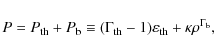
where the thermal energy density,

The sound speed, required for the approximate Riemann solver and for the determination of the time step, is given by
We used
6.1.2 Initial conditions
With presently available computational resources it is not possible to perform global simulations of the close encounter or merging of two magnetized neutron stars with a grid resolution sufficiently high to resolve also the growth of KH instabilities in shearing magnetized neutron star matter. Nevertheless one can study some aspects of this phenomenon by means of local simulations covering only a small volume around the shear layer.
To this end we consider a quadratic (2D) / cubic (3D) computational domain in Cartesian coordinates assuming that the x-axis is parallel to the direction of the shear flow, the y-axis parallel to the line connecting the centers of the two neutron stars, and the z-axis (in 3D) perpendicular to that line. As the edges of our computational domain have a size of 200 m only, i.e., they are much smaller than the radius of a neutron star, we consider only homogeneous initial states, i.e, initial models with constant density and pressure. Besides the shear flow in x-direction the initial models are static, too. This approximation is justified as the merging neutron stars move much faster in x-direction than they approach each other in y-direction due to the action of gravity. Accordingly, we use periodic boundary conditions in x and z-direction, and reflecting ones in y-direction.
The shear velocity vx, corresponding to either a Mach number of
![]() or
or
![]() ,
has the same
,
has the same ![]() -profile as that used
in the simulations of the previous sections, and we also consider both
parallel and anti-parallel initial magnetic field configurations. The
shear velocity is supposed to mimic the orbital velocity of the two
neutron stars. We trigger the instability by applying similar
perturbations as in the previous sections, i.e., a combination of a
sinusoidal and a random velocity perturbation.
-profile as that used
in the simulations of the previous sections, and we also consider both
parallel and anti-parallel initial magnetic field configurations. The
shear velocity is supposed to mimic the orbital velocity of the two
neutron stars. We trigger the instability by applying similar
perturbations as in the previous sections, i.e., a combination of a
sinusoidal and a random velocity perturbation.
6.2 Two-dimensional models
A number of models (see Table A.6) computed in two dimensions confirm the basic results discussed in the previous sections, i.e., the occurrence of three phases, namely KH growth, kinematic amplification, and saturation. This also holds for the dependence of the parameters characterizing these phases, e.g., the termination values of the field strength and magnetic energ, on the initial data and the grid resolution.
We performed simulations with up to 20482 zones. The width of the
shear layer was a = 10 m, and the initial velocity
vx0 = 1.83or
![]() cms/s, for models with
cms/s, for models with
![]() or
or
![]() ,
respectively. Due to the affordable grid resolution we employed
rather strong initial fields of the order of
,
respectively. Due to the affordable grid resolution we employed
rather strong initial fields of the order of
![]() G,
corresponding to Alfvén numbers
G,
corresponding to Alfvén numbers
![]() .
The initial field was either
parallel or anti-parallel to the shear flow.
.
The initial field was either
parallel or anti-parallel to the shear flow.
We start the discussion with models with
![]() .
The KH
instability developed within less than 0.05 ms, establishing one
large KH vortex. Afterwards, the magnetic field is amplified
kinematically by the vortical flow. The physics of KH growth
termination is the same as that described in Sect. 4.3.
Hence, we also find a similar dependence for the field amplification
factor
.
The KH
instability developed within less than 0.05 ms, establishing one
large KH vortex. Afterwards, the magnetic field is amplified
kinematically by the vortical flow. The physics of KH growth
termination is the same as that described in Sect. 4.3.
Hence, we also find a similar dependence for the field amplification
factor
![]() on the initial field strength and the grid
resolution.
on the initial field strength and the grid
resolution.
- On finer grids one can resolve the increasingly thin structures of the magnetic field better. Consequently, one finds more efficient amplification, until for a sufficiently fine grid convergence of the amplification factor is achieved.
- Weaker initial fields are amplified by a larger amount, i.e., the maximum value of the field strength at the end of the KH growth phase depends only weakly on the initial field (assuming numerical convergence). The total magnetic energy increases with increasing initial field strength due to the larger volume filling factor of magnetic flux tubes for stronger initial fields.
Models with
![]() G and
G and
![]() G reach slightly fluctuating maximum field strengths around
G reach slightly fluctuating maximum field strengths around
![]() G in the saturated state. The volume filling
factor of the magnetic field, i.e., the relative volume occupied by
intense magnetic flux tubes, decreases with decreasing initial field
strength leading to a weaker mean magnetic field and consequently a
slower deceleration of the shear flow for weaker initial fields. We
find mean fields of
G in the saturated state. The volume filling
factor of the magnetic field, i.e., the relative volume occupied by
intense magnetic flux tubes, decreases with decreasing initial field
strength leading to a weaker mean magnetic field and consequently a
slower deceleration of the shear flow for weaker initial fields. We
find mean fields of ![]()
![]() G and
G and ![]()
![]() G for
b0x = 1014 G and
G for
b0x = 1014 G and
![]() G,
respectively. The time scale for deceleration of the shear flow is
less than 1 millisecond. For a model with an initial field of
G,
respectively. The time scale for deceleration of the shear flow is
less than 1 millisecond. For a model with an initial field of
![]() G, the deceleration is sufficiently rapid to cause a
significant decay (by about an order of magnitude) of the turbulent
energy within 0.5 ms.
G, the deceleration is sufficiently rapid to cause a
significant decay (by about an order of magnitude) of the turbulent
energy within 0.5 ms.
The evolution of the shear layer is affected by the choice of the
initial field configuration. Parallel initial fields have, similarly
to our observations above, a somewhat larger impact on the dynamics of
the KH instability. In this case, the non-vanishing magnetic flux
threading surfaces
![]() is conserved due to the boundary
conditions, and gives rise to an effective driving force. Apart from
lacking this additional driver, anti-parallel magnetic fields are
prone to stronger dissipation due to presence of stronger currents at
the boundaries between regions of opposite magnetic polarity.
is conserved due to the boundary
conditions, and gives rise to an effective driving force. Apart from
lacking this additional driver, anti-parallel magnetic fields are
prone to stronger dissipation due to presence of stronger currents at
the boundaries between regions of opposite magnetic polarity.
The evolution of models with a supersonic shear flow (
![]() )
is
similar to that of their dimensionless conterparts discussed
previously. With initial fields between 10 and
)
is
similar to that of their dimensionless conterparts discussed
previously. With initial fields between 10 and
![]() ,
the initial Alfvén numbers of the shear flow are
between
,
the initial Alfvén numbers of the shear flow are
between ![]() 110 and
110 and ![]() 440, i.e., in the range covered in
Sect. 4.4. The dynamics is the same: pressure waves steepen
into oblique shocks, and the dissipation of kinetic into thermal
energy in these shocks creates a broad transition layer between the
two regions of positive and negative vx. The shear flow is
decelerated very efficiently even for very weak fields. We find
3field amplification up to
440, i.e., in the range covered in
Sect. 4.4. The dynamics is the same: pressure waves steepen
into oblique shocks, and the dissipation of kinetic into thermal
energy in these shocks creates a broad transition layer between the
two regions of positive and negative vx. The shear flow is
decelerated very efficiently even for very weak fields. We find
3field amplification up to
![]() for
the maximum field strength and
for
the maximum field strength and
![]() for the volume-averaged rms value of the field,
for the volume-averaged rms value of the field,
![]() ,
i.e., of the
same order as in the case
,
i.e., of the
same order as in the case
![]() but systematically higher by a
factor
but systematically higher by a
factor ![]() 2, with considerably higher values for parallel than for
anti-parallel initial fields.
2, with considerably higher values for parallel than for
anti-parallel initial fields.
Hence, the results and in particular their dependence on the physical and numerical parameters of the models explored in Sect. 4, are robust with respect to the described variations of the initial conditions. Consequently, we can expect them to apply to merger systems without too strong modifications.
6.3 Three-dimensional models
One of the main questions to be addressed by 3D simulations is whether the dynamics of these models is dominated by magnetic flux tubes or by 3D hydrodynamic instabilities. As we have seen in the previous sections, this has a distinct influence on, e.g., the magnetic field strength achieved at saturation.
For the 3D simulations we used grids of up to
![]() zones. The initial field strength was between 5 and
zones. The initial field strength was between 5 and
![]() G. We again applied different combinations of
sinusoidal and random velocity perturbations to the shear layer.
G. We again applied different combinations of
sinusoidal and random velocity perturbations to the shear layer.
The models (see Table A.7) show the same overall dynamics and the same evolutionary phases as the corresponding models discussed in Sect. 4. We find the initial KH growth phase, the kinematic amplification phases, followed by the development of parasitic instabilities leading to a non-linear saturated state. The flow during the first two phases is very similar to that in 2D, and field amplification follows the same trends with initial field and grid resolution as outlined above. The further evolution depends, as discussed above, strongly on the relative amplitude of random and sinusoidal perturbations.
When a small random perturbation is imposed, field amplification
proceeds through the first two growth phases the field strength being
limited by its back reaction onto the flow. These models suffer (if
resolved well on a sufficiently fine grid) hydromagnetic instabilities
of the flux sheet, leading to the break-up of the KH vortex tube and
the deceleration of the shear flow. For a well-resolved model with
![]() G the maximum magnetic field strength is
G the maximum magnetic field strength is
![]()
![]() G, while the rms maximum is only
G, while the rms maximum is only
![]()
![]() G.
G.
For models with large random perturbations and for models with very
weak initial fields the disruption of the KH vortex tube is
predominantly due to hydrodynamic instabilities leading to a very
efficient deceleration of the shear flow. These instabilities grow on
a very short time scale, causing a strong growth of the
volume-averaged transverse kinetic energy densities
![]() and
and
![]() ,
as well as of all volume-averaged magnetic
energy densities (
,
as well as of all volume-averaged magnetic
energy densities (
![]() ,
and
,
and
![]() ).
).
The amplification factors are similar for all components of the field, leading to equipartition among them at peak magnetic energy. The amplification rate is at first very large but decreases strongly as the parasitic instabilities saturate. Eventually, the magnetic energy reaches a maximum, and then starts to decrease again. This maximum depends either on the grid resolution (for the most weakly magnetized models), or on the dynamic back-reaction of the field onto the flow. In the latter case, field amplification ceases once the volume-averaged transverse kinetic energy densities (decaying from their maximum values at saturation of the parasitic instabilities) decrease to roughly the level of the volume-averaged magnetic energy density.
The magnetic field is amplified during all three growth phases: at the
KH growth rate during the KH growth phase, at a (smaller) rate
determined by the overturning velocity of the KH vortex tube during
the kinematic amplification phase, and during the growth of the
parasitic instabilities. Since the magnetic field starts to decrease
shortly after saturation of the parasitic instabilities feeding off
the shear flow, the maximum field strength is reached at that moment.
The magnetic field energy can reach at most equipartition with the
(decaying) transverse kinetic energy, which typically has a value of
![]() 1043 erg. For a model with
1043 erg. For a model with
![]() G
the corresponding root mean square saturation field is
G
the corresponding root mean square saturation field is ![]()
![]() G. The weaker the initial field, the smaller is the maximum
magnetic energy, since the achievable amplification factor is limited
by the duration of the three field amplification phases. The maximum
field strength reached anywhere in the computational domain depends
only weakly on the initial field, and has a value between 6 and
G. The weaker the initial field, the smaller is the maximum
magnetic energy, since the achievable amplification factor is limited
by the duration of the three field amplification phases. The maximum
field strength reached anywhere in the computational domain depends
only weakly on the initial field, and has a value between 6 and
![]() G.
G.
The decay of the turbulence (measured by the transverse kinetic and
magnetic energy densities) as well as that of the shear flow starts at
a similar rate for all models, and the magnetic field decreases much
faster than it does in the corresponding 2D models. Shortly after
(![]() 0.05 ms) the rms field strength as well as the total
field strength reach their peak values early during the saturation
phase, the kinetic energy densities decay very rapidly, and much
faster than the magnetic energy density. The decay slows down shortly
after
0.05 ms) the rms field strength as well as the total
field strength reach their peak values early during the saturation
phase, the kinetic energy densities decay very rapidly, and much
faster than the magnetic energy density. The decay slows down shortly
after
![]() has decreased below the
value of
has decreased below the
value of
![]() .
Afterwards, all transverse energy
densities decay at a similar rate. In the more strongly magnetized
models this happens when
.
Afterwards, all transverse energy
densities decay at a similar rate. In the more strongly magnetized
models this happens when
![]() (which can undergo a phase
of particularly fast decay) is still larger than
(which can undergo a phase
of particularly fast decay) is still larger than
![]() ,
whereas it is usually the other way round for
weaker initial fields (a similar effect can be observed for
under-resolved models where insufficient grid resolution limits the
field amplification). During the further evolution the relative sizes
of
,
whereas it is usually the other way round for
weaker initial fields (a similar effect can be observed for
under-resolved models where insufficient grid resolution limits the
field amplification). During the further evolution the relative sizes
of
![]() ,
,
![]() ,
and
,
and
![]() remain unchanged.
remain unchanged.
For weak initial fields, (b0x = 1, 5, and
![]() G, the kinetic energy density dominates the magnetic one by
a factor
G, the kinetic energy density dominates the magnetic one by
a factor ![]() 2.7 in the final state. Concerning the
volume-averaged kinetic energy densities we find
2.7 in the final state. Concerning the
volume-averaged kinetic energy densities we find
![]() .
This relation
also holds for the volume-averaged magnetic energy densities,
indicating a relatively high degree of isotropy of the turbulence.
The final state for
.
This relation
also holds for the volume-averaged magnetic energy densities,
indicating a relatively high degree of isotropy of the turbulence.
The final state for
![]() G is shown in the left
panel of Fig. 22. Obviously, neither the flow nor
the magnetic field show any preferred direction. Instead, one
recognizes a complex pattern of tangled small-scale flux tubes.
G is shown in the left
panel of Fig. 22. Obviously, neither the flow nor
the magnetic field show any preferred direction. Instead, one
recognizes a complex pattern of tangled small-scale flux tubes.
For sufficiently strong initial fields (
b0x = 20, and
![]() G), the final state is more strongly magnetized. As the
turbulent energy decays more rapidly than the x-component of the
magnetic field, bx dominates the dynamics after
G), the final state is more strongly magnetized. As the
turbulent energy decays more rapidly than the x-component of the
magnetic field, bx dominates the dynamics after
![]() ms leading to a slower deceleration of the shear flow and a
more pronounced alignment of flow features (flux and vorticity tubes)
in x-direction (see Fig. 22, right panel).
ms leading to a slower deceleration of the shear flow and a
more pronounced alignment of flow features (flux and vorticity tubes)
in x-direction (see Fig. 22, right panel).
Similarly to the 2D models discussed above, a parallel initial
magnetic field has a stronger influence on the dynamics than an
anti-parallel one: the field strength reaches a higher maximum value,
and the influence of hydrodynamic instabilities is slightly less. At
late stages, such models may exhibit a phase of hydromagnetic
deceleration, in contrast to the roughly constant value of
![]() in models with strong anti-parallel initial fields.
in models with strong anti-parallel initial fields.
For of supersonic shear flows with
![]() ,
the evolution is
similar to that of the dimensionless models discussed in
Sect. 5.2. We find a fast growth of 3D hydrodynamic
instabilities disrupting the shear flow before the shock-mediated
mechanism working in 2D can operate. Turbulence sets in quickly
without the intermediate development of a KH vortex, and the shear
flow is decelerated very efficiently. The maximum magnetic fields we
find are of the order of
,
the evolution is
similar to that of the dimensionless models discussed in
Sect. 5.2. We find a fast growth of 3D hydrodynamic
instabilities disrupting the shear flow before the shock-mediated
mechanism working in 2D can operate. Turbulence sets in quickly
without the intermediate development of a KH vortex, and the shear
flow is decelerated very efficiently. The maximum magnetic fields we
find are of the order of
![]() for the
absolute maximum, and
for the
absolute maximum, and
![]() for the
rms field, respectively. These values are rather insensitive to
the initial field strength and geometry.
for the
rms field, respectively. These values are rather insensitive to
the initial field strength and geometry.
7 Summary and conclusions
Global simulations indicate that the contact layer between two merging neutron stars is a site of very efficient field amplification. The layer is prone to the Kelvin-Helmholtz instability, and thus, exponential growth of any weak seed field is possible, as observed by Price & Rosswog (2006) (see also Liu et al. 2008; Anderson et al. 2008; Giacomazzo et al. 2009). The limitations of their simulations, mainly concerning grid resolution, did not allow these authors to determine the saturation level of the instability firmly and accurately. Thus, the implications of magnetic fields for the merger dynamics remains unclear. On the basis of energetic arguments, the instability might lead to a field in equipartition with the kinetic or the internal energy of the shear flow, corresponding to field strengths of the order of 1016 G or 1018 G, respectively.
We reassessed these arguments by means of local high-resolution simulations of magnetized shear layers in two and three spatial dimensions. To this end we performed more than 220 simulations focusing on properties of the hydromagnetic KH instability in general as well as on the contact surfaces of merging neutron stars. We refer to these two classes of simulations as dimensionless and merger-motivated models, respectively.
We employed a recently developed multi-dimensional Eulerian finite-volume ideal MHD code based on high-order spatial reconstruction techniques and Riemann solvers of the MUSTA-type (Obergaulinger 2008; Obergaulinger et al. 2009).
We set up a KH-unstable shear flow in Cartesian coordinates in a quadratic (2D) and cubic (3D) computational domain imposing periodic boundary conditions in the direction of the shear flow and reflecting or open ones in the transverse directions. Focusing on the effects of a magnetic field on the instability, we used a simplified equation of state (ideal gas EOS and a hybrid barotropic/ideal gas EOS for the dimensionless and the merger-motivated models, respectively) and neglected additional physics, e.g., such as neutrino transport.
Under these simplifications, the shear flows are characterized by two
parameters, the initial Mach number
![]() and the initial Alfvén
number
and the initial Alfvén
number
![]() ,
measuring the magnitude of the jump in shear velocity
in units of the sound speed and the Alfvén velocity, respectively.
,
measuring the magnitude of the jump in shear velocity
in units of the sound speed and the Alfvén velocity, respectively.
Analytic considerations and previous simulations of non-magnetized
shear flows show that the growth rate of the KH instability as well as
its saturation level (i.e., the kinetic energy of the circular KH
vortex formed by the instability) increase with increasing
![]() for
subsonic shear flows . A magnetic field is known to reduce the growth
rate and potentially, i.e., for
for
subsonic shear flows . A magnetic field is known to reduce the growth
rate and potentially, i.e., for
![]() ,
even to suppress the
instability (Miura & Pritchett 1982; Keppens et al. 1999; Chandrasekhar 1961). However, less is known about the
saturation level and the dynamic back-reaction, in particular for weak
initial fields.
,
even to suppress the
instability (Miura & Pritchett 1982; Keppens et al. 1999; Chandrasekhar 1961). However, less is known about the
saturation level and the dynamic back-reaction, in particular for weak
initial fields.
Frank et al. (1996); Jones et al. (1997); Jeong et al. (2000); Ryu et al. (2000) studied the evolution of the hydromagnetic KH instability in two and three dimensions. In 2D, models undergo a transition from non-linear stabilization of the KH vortex to its violent disruption or more gradual dissipation when the initial field strength is reduced, while in 3D purely hydrodynamic elliptic instabilities of the vortex tube may dominate over MHD effects.
The study of these non-linear effects is hampered by high requirements
on the grid resolution that is necessary to follow the development of
increasingly thin magnetic flux sheets and tubes. This limits the
range of Alfvén numbers for which numerical convergence can be
achieved to rather modest values. It also reduces the predictive power
for merger systems, where rather weak initial fields are expected.
This limitation can be overcome only when using large grids in
combination with a highly accurate code. We evolved subsonic,
transsonic, and supersonic shear flows with
![]() ,
while using the maximum Alfvén numbers for which convergence is
achievable. The resulting broad range of Alfvén numbers covered by
our simulations allows us to establish scaling laws governing the
field amplification as a function of the initial field strength.
,
while using the maximum Alfvén numbers for which convergence is
achievable. The resulting broad range of Alfvén numbers covered by
our simulations allows us to establish scaling laws governing the
field amplification as a function of the initial field strength.
The main results of our simulations are:
- 1.
- In 2D, we confirm the results of analytic work (in the linear regime) and previous simulations concerning the growth rate and the saturation of the transverse kinetic energy densities for strong initial fields due to Miura & Pritchett (1982); Keppens et al. (1999); Chandrasekhar (1961). This agreement supports the viability of our numerical approach for the problem at hand.
- 2.
- For subsonic shear flows (
 )
we explored a wide
range of initial field strengths covering Alfvén numbers up to
)
we explored a wide
range of initial field strengths covering Alfvén numbers up to
 in 2D.
- (a)
- For intermediate and weak fields, we distinguish two phases: the KH growth phase during which the field grows at the KH growth rate, and after formation of a KH vortex, a phase of kinematic field amplification by the overturning vortex. The growth rate during the latter phase depends on the velocity of the vortex. The field is highly intermittent and concentrated in flux sheets, which are stretched by the flow leading to an exponential growth of the field strength while the sheet width decreases.
- (b)
- The termination of the kinematic amplification phase occurs either numerically, when the flux sheets get too thin to be resolved on a given computational grid, or dynamically by back-reaction of the field onto the flow. The most important mode of back-reaction is the growth of secondary resistive instabilities feeding off the magnetic energy of the flux sheets. These instabilities terminate the kinematic field growth and initiate the non-linear saturation phase during which the KH vortex is destroyed by the ensuing MHD turbulence and the shear flow is gradually decelerated. This scenario is equivalent to that of the disruption models of Frank et al. (1996).
- (c)
- We quantified the amount of field amplification during the
kinematic amplification phase by computing the ratio of the
volume-averaged Maxwell stress component Mxy at the beginning
and at the end of that phase. The amplification factor scales
with the initial Alfvén number as
 ,
corresponding
to a scaling of the maximum Maxwell stress with the initial field
strength as b05/4. If the simulation is under-resolved, the
amplification factor is reduced by a factor
,
corresponding
to a scaling of the maximum Maxwell stress with the initial field
strength as b05/4. If the simulation is under-resolved, the
amplification factor is reduced by a factor
 (m being the number of zones per dimension). The maximum local field
strength corresponds to a local equipartition between the
magnetic energy density of a flux sheet and the kinetic energy
density of the shear flow; it depends only weakly on the initial
field.
(m being the number of zones per dimension). The maximum local field
strength corresponds to a local equipartition between the
magnetic energy density of a flux sheet and the kinetic energy
density of the shear flow; it depends only weakly on the initial
field.
- (d)
- The secondary resistive instabilities observed in our
simulations are triggered by numerical resistivity instead of a
physical one. The numerical resistivity, which is a function of
the grid resolution
 ,
is important only for small thin
structures having a spatial size of the order of
or less.
In our simulations, it causes current sheets to become unstable
when their width approaches the grid spacing .
Although
only simulations with arbitrarily high resolution can sustain
arbitrarily thin and intense current sheets, we observe
nevertheless convergence: the field amplification becomes
independent of the grid resolution, if
is smaller than
some threshold which depends on the initial field strength. The
reason for this independence is the fact that the most unstable
current sheets do not consist of individual flux sheets but of
pairs or triples of coalescing flux sheets. Thus, decreasing the
distance between flux sheets does not lead to a stronger field
(which would be the case, if a single flux sheet is compressed in
transverse direction).
,
is important only for small thin
structures having a spatial size of the order of
or less.
In our simulations, it causes current sheets to become unstable
when their width approaches the grid spacing .
Although
only simulations with arbitrarily high resolution can sustain
arbitrarily thin and intense current sheets, we observe
nevertheless convergence: the field amplification becomes
independent of the grid resolution, if
is smaller than
some threshold which depends on the initial field strength. The
reason for this independence is the fact that the most unstable
current sheets do not consist of individual flux sheets but of
pairs or triples of coalescing flux sheets. Thus, decreasing the
distance between flux sheets does not lead to a stronger field
(which would be the case, if a single flux sheet is compressed in
transverse direction).
- (e)
- The disruption of the vortex and the efficient dissipation set these resisto-dynamic models apart from the class of dissipation models with even weaker initial fields where the KH vortex remains intact, and only very slow dissipation is provided by turbulence. In the simulations of Frank et al. (1996), secondary instabilities do not modify the flow field qualitatively. Our simulations indicate that this is, partially at least, a resolution effect. If a simulation is under-resolved and the field growth is not limited by dynamic back-reaction but by the resolvable width of flux sheets, no disruption will occur, and the deceleration time of the shear flow is very long. Converged simulations show, on the other hand, the disruption of the KH vortex by secondary magnetic instabilities when the magnetic field strength approaches a local maximum close to equipartition with the kinetic energy density of the shear flow. This happens in all converged models, but for weak initial fields, the deceleration time can be very long.
- (f)
- Models with initially anti-parallel and parallel magnetic fields, but otherwise identical, give qualitatively similar results, the above discussed effects being somewhat less pronounced in case of the former field configuration.
- 3.
- The contact layer of merging neutron stars resembles supersonic shear flows. In principle, these are stable. We find, however, that an exponentially growing instability may occur when closed boundary conditions are imposed in the direction transverse to the shear flow. The instability is mediated by shock waves traveling through the computational domain. The corresponding growth rates are much smaller than for subsonic shear flows. The effects of a magnetic field on a supersonic shear flow are qualitatively similar to those on subsonic shear flows.
- 4.
- In 3D the disruption of the KH vortex tube can be induced by a
purely hydrodynamic secondary so-called elliptic instability
as discussed, e.g., by Ryu et al. (2000). It
leads to a very rapid growth of the kinetic energy densities
corresponding to all components of the flow velocity once the KH
vortex tube forms, and decelerates the shear flow more efficiently
than the MHD mechanisms outlined above. Which of the two possible
disruption mechanisms, elliptic or hydromagnetic, operates depends
on the initial field strength b0 and the value of volume-averaged
kinetic energy density
 .
The magnetic mechanism
will dominate only if
,
i.e., as
long as the magnetic energy density exceeds the transverse kinetic
energy in z-direction. Due to the very fast growth of the
elliptic instability, this may be the case only for a short time, if
at all. A rather strong initial field and small perturbations in
z-direction are required for a hydromagnetic disruption.
.
The magnetic mechanism
will dominate only if
,
i.e., as
long as the magnetic energy density exceeds the transverse kinetic
energy in z-direction. Due to the very fast growth of the
elliptic instability, this may be the case only for a short time, if
at all. A rather strong initial field and small perturbations in
z-direction are required for a hydromagnetic disruption.
- 5.
- 2D and 3D simulations of shear flows with merger-motivated
initial conditions performed in a cubic computational domain of
constant density and pressure having an edge size of 200 m show
the same overall dynamics as corresponding dimensionless models.
The initial Mach number of the shear flow was chosen to be
 and
and
 corresponding to a density of 1013 g cm-3, and shear velocities of
 cm/s, and
 cm/s, respectively. The initial magnetic field
strength was varied between
cm/s, respectively. The initial magnetic field
strength was varied between
 G and
G and
 G.
G.
- (a)
- The instability grows rapidly: saturation occurs within
 0.1 ms, and the disruption and deceleration times
are much less than 1 ms.
0.1 ms, and the disruption and deceleration times
are much less than 1 ms.
- (b)
- The dynamics is the same as that of the dimensionless models.
Field amplification leads to a maximum field strength 1016 G, and a rms value of
 G. These values are the same for 3D models suffering
hydrodynamic and hydromagnetic disruption.
G. These values are the same for 3D models suffering
hydrodynamic and hydromagnetic disruption.
Instead, local equipartition with the kinetic energy density is
reached with corresponding maximum fields ![]() 1016 G, as
speculated by Price & Rosswog (2006).
Due to the high degree of intermittency in the case of weak initial
fields, the (rms) average of the field strength is smaller, i.e,
its direct dynamic impact (e.g., disruption of the KH vortex tube or
deceleration of the shear flow) on the flow is probably rather
limited. This is even more the case if the geometry of the system and
the perturbations resulting from the merger dynamics enhance the
importance of purely hydrodynamic instabilities. More indirect
effects can, however, not be excluded, e.g., whether magnetic flux
tubes created at the shear layer are transported rapidly far away by
large-scale flows. The short period of time during which the magnetic
field stays close to its maximum value and its fast decay impose
severe constraints on the impact that the amplified fields may have on
any hydromagnetic or electromagnetic jet-launching mechanism in a
merger of two neutron stars. We note that magnetically driven
relativistic outflows may need much longer time scales (
1016 G, as
speculated by Price & Rosswog (2006).
Due to the high degree of intermittency in the case of weak initial
fields, the (rms) average of the field strength is smaller, i.e,
its direct dynamic impact (e.g., disruption of the KH vortex tube or
deceleration of the shear flow) on the flow is probably rather
limited. This is even more the case if the geometry of the system and
the perturbations resulting from the merger dynamics enhance the
importance of purely hydrodynamic instabilities. More indirect
effects can, however, not be excluded, e.g., whether magnetic flux
tubes created at the shear layer are transported rapidly far away by
large-scale flows. The short period of time during which the magnetic
field stays close to its maximum value and its fast decay impose
severe constraints on the impact that the amplified fields may have on
any hydromagnetic or electromagnetic jet-launching mechanism in a
merger of two neutron stars. We note that magnetically driven
relativistic outflows may need much longer time scales (![]() a few ms) to tap the rotational energy of either the black hole or the
accretion disk resulting after the merger.
a few ms) to tap the rotational energy of either the black hole or the
accretion disk resulting after the merger.
Though these results limit the prospect for magnetic effects to play a dynamic role in neutron star mergers, their proper inclusion in current and forthcoming simulations may be necessary, because magnetic fields influence the dissipation rates in the shear layer, i.e., their neglect may lead to an underestimation of the temperature in the shear layer, and hence in the accretion disk. Given the resolution requirements imposed by weak initial fields, a more sophisticated treatment of the problem probably also has to abandon the assumption of ideal MHD and to consider the formulation of a turbulence model for unresolved magnetic field structures.
AcknowledgementsThis research has been supported by the Spanish Ministerio de Educación y Ciencia (grants AYA2007-67626-C03-01, CSD2007-00050), and by the Collaborative Research Center on Gravitational Wave Astronomy of the Deutsche Forschungsgemeinschaft (DFG SFB/Transregio 7). MAA is a Ramón y Cajal fellow of the Ministerio de Educación y Ciencia. Most of the simulations were performed at the Rechenzentrum Garching (RZG) of the Max-Planck-Society. We are also thankful for the computer resources, the technical expertise, and the assistance provided by the Barcelona Supercomputing Center - Centro Nacional de Supercomputación. Parts of this article have been written during M.O.'s visit to the Departamento de Astronomía y Astrofísica of the Universidad de Valencia. He wants to express his gratitude for the kind hospitality experienced there.
Appendix A: Tables of models
We provide tables listing the parameters and important properties of the models computed:
- Table A.1
- lists the parameters of models which we computed to compare the growth rates obtained numerically with theoretical predictions, serving as code validation.
- Table A.2
- lists 2D hydrodynamic models of transonic and supersonic shear flows.
- Tables A.3
- and A.4 list the amplification factors of the magnetic field and the disruption and deceleration rates of models with weak initial fields, respectively.
- Table A.5
- lists the initial data of 3D dimensionless models.
- Tables A.6 and A.7
- list the initial conditions of 2D and 3D merger-motivated models, respectively.
Table A.1: Summary of models computed to compare numerical growth rates with theoretical predictions.
Table A.2: Summary of 2D hydrodynamic supersonic models.
Table A.3: Initial data and amplification factors of the weak-field models.
Table A.4: Disruption time and deceleration rate of weak-field models.
Table A.5: List of 3D models.
Table A.6: List of 2D merger-motivated models simulated on grids of 10242 and 20482 zones, respectively.
Table A.7: Same as Table A.6 but for the 3D merger-motivated models simulated on grids of 1283 and 2563 zones, respectively.
References
- Agertz, O., Moore, B., Stadel, J., et al. 2007, MNRAS, 380, 963 [NASA ADS] [CrossRef] [Google Scholar]
- Anderson, M., Hirschmann, E. W., Lehner, L., et al. 2008, Phys. Rev. Lett., 100, 191101 [NASA ADS] [CrossRef] [PubMed] [Google Scholar]
- Baty, H., Keppens, R., & Comte, P. 2003, Phys. Plas., 10, 4661 [Google Scholar]
- Biskamp, D. 2000, Magnetic Reconnection in Plasmas (Cambridge, UK: Cambridge University Press), Cambridge monographs on plasma physics, 3 [Google Scholar]
- Chandrasekhar, S. 1961, Hydrodynamic and hydromagnetic stability, International Series of Monographs on Physics (Oxford: Clarendon) [Google Scholar]
- Evans, C. R., & Hawley, J. F. 1988, ApJ, 332, 659 [Google Scholar]
- Frank, A., Jones, T. W., Ryu, D., et al. 1996, ApJ, 460, 777 [NASA ADS] [CrossRef] [Google Scholar]
- Gardiner, T. A., & Stone, J. M. 2005, J. Comput. Phys., 205, 509 [Google Scholar]
- Gardiner, T. A., & Stone, J. M. 2008, J. Comput. Phys., 227, 4123 [NASA ADS] [CrossRef] [Google Scholar]
- Giacomazzo, B., Rezzolla, L., & Baiotti, L. 2009, MNRAS, 399, L164 [NASA ADS] [Google Scholar]
- Harten, A. 1983, J. Comput. Phys., 49, 357 [NASA ADS] [CrossRef] [MathSciNet] [Google Scholar]
- Iroshnikov, P. S. 1964, SvA, 7, 566 [Google Scholar]
- Jeong, H., Ryu, D., Jones, T. W., et al. 2000, ApJ, 529, 536 [NASA ADS] [CrossRef] [Google Scholar]
- Jones, T. W., Gaalaas, J. B., Ryu, D., et al. 1997, ApJ, 482, 230 [NASA ADS] [CrossRef] [Google Scholar]
- Keil, W., Janka, H.-T., & Müller, E. 1996, ApJ, 473, L111 [NASA ADS] [CrossRef] [Google Scholar]
- Keppens, R., Tóth, G., Westermann, R. H. J., et al. 1999, J. Plasma Phys., 61, 1 [NASA ADS] [CrossRef] [Google Scholar]
- Kraichnan, R. H. 1965, Phys. Fluids, 8, 1385 [Google Scholar]
- LeVeque, R. J. 1992, Numerical Methods for Conservation Laws, 2nd edn., Lectures in mathematics - ETH Zürich (Birkhäuser) [Google Scholar]
- Levy, D., Puppo, G., & Russo, G. 2002, SIAM J. Sci. Comput., 24, 480 [CrossRef] [Google Scholar]
- Liu, X.-D., Osher, S., & Chan, T. 1994, J. Comput. Phys., 115, 200 [NASA ADS] [CrossRef] [MathSciNet] [Google Scholar]
- Liu, Y. T., Shapiro, S. L., Etienne, Z. B., et al. 2008, Phys. Rev. D, 78, 024012 [NASA ADS] [CrossRef] [Google Scholar]
- Londrillo, P., & del Zanna, L. 2004, J. Comput. Phys., 195, 17 [NASA ADS] [CrossRef] [Google Scholar]
- Miura, A., & Pritchett, P. L. 1982, J. Geophys. Res., 87, 7431 [NASA ADS] [CrossRef] [Google Scholar]
- Monaghan, J. J. 1992, ARA&A, 30, 543 [NASA ADS] [CrossRef] [Google Scholar]
- Obergaulinger, M. 2008, Ph.D. Thesis, Technische Universität München [Google Scholar]
- Obergaulinger, M., Cerdá-Durán, P., Müller, E., et al. 2009, A&A, 498, 241 [NASA ADS] [CrossRef] [EDP Sciences] [Google Scholar]
- Oechslin, R., Janka, H.-T., & Marek, A. 2007, A&A, 467, 395 [NASA ADS] [CrossRef] [EDP Sciences] [Google Scholar]
- Orszag, S. A., & Tang, C.-M. 1979, J. Fluid Mech., 90, 129 [NASA ADS] [CrossRef] [Google Scholar]
- Price, D. J., & Rosswog, S. 2006, Science, 312, 719 [NASA ADS] [CrossRef] [PubMed] [Google Scholar]
- Rosswog, S. 2007, in Rev. Mex. Astron. Astrofis. Conf. Ser., 27, 57 [Google Scholar]
- Ryu, D., & Jones, T. W. 1995, ApJ, 442, 228 [NASA ADS] [CrossRef] [Google Scholar]
- Ryu, D., Jones, T. W., & Frank, A. 2000, ApJ, 545, 475 [NASA ADS] [CrossRef] [Google Scholar]
- Suresh, A., & Huynh, H. 1997, J. Comput. Phys., 136, 83 [NASA ADS] [CrossRef] [Google Scholar]
- Titarev, V. A., & Toro, E. F. 2005, Int. J. Numer. Meth. Fluids, 49, 117 [Google Scholar]
- Toro, E. F., & Titarev, V. A. 2006, J. Comput. Phys., 216, 403 [NASA ADS] [CrossRef] [Google Scholar]
Footnotes
- ...
following
![[*]](/icons/foot_motif.png)
- Without elaborating in more detail, we note that a similar result holds for magnetized models.
- ...
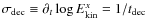
- We also considered alternative definitions of
 that, however, do not change the arguments in the discussion below.
All Tables
Table A.1: Summary of models computed to compare numerical growth rates with theoretical predictions.
Table A.2: Summary of 2D hydrodynamic supersonic models.
Table A.3: Initial data and amplification factors of the weak-field models.
Table A.4: Disruption time and deceleration rate of weak-field models.
Table A.5: List of 3D models.
Table A.6: List of 2D merger-motivated models simulated on grids of 10242 and 20482 zones, respectively.
Table A.7: Same as Table A.6 but for the 3D merger-motivated models simulated on grids of 1283 and 2563 zones, respectively.
All Figures
![\begin{figure}
\par\includegraphics[width=7.2cm,clip]{13386F01a}
\end{figure}](/articles/aa/full_html/2010/07/aa13386-09/img87.png)
|
Figure 1:
Linear growth phase of the KH instability in model grw-3. The solid black line shows the volume-averaged kinetic energy
density
|
| In the text | |
![\begin{figure}
\par\includegraphics[width=7.2cm,clip]{13386F02a}
\includegraphics[width=7.2cm,clip]{13386F02b}
\end{figure}](/articles/aa/full_html/2010/07/aa13386-09/img89.png)
|
Figure 2:
Logarithm of the modulus of the flow vorticity and the velocity field (vectors) of a non-magnetic model with
|
| In the text | |
![\begin{figure}
\par\includegraphics[width=8cm,clip]{13386F03a}
\end{figure}](/articles/aa/full_html/2010/07/aa13386-09/img103.png)
|
Figure 3:
Volume averaged kinetic energy density
|
| In the text | |
![\begin{figure}
\par\includegraphics[width=7.2cm,clip]{13386F04a}\vspace*{3.4mm}
\end{figure}](/articles/aa/full_html/2010/07/aa13386-09/img113.png)
|
Figure 4:
Volume averaged transverse kinetic (solid) and magnetic (dashed) energy densities
|
| In the text | |
|
|
Figure 5:
Growth of the volume-averaged turbulent (transverse)
magnetic energy density
|
| In the text | |
![\begin{figure}
\par\includegraphics[width=6.4cm,clip]{13386F06a} %
\end{figure}](/articles/aa/full_html/2010/07/aa13386-09/img117.png)
|
Figure 6:
Snapshot of a model with initial Mach number
|
| In the text | |
|
|
Figure 7: Snapshot of the source term of the total magnetic energy density (Eq. (13)) for the model shown in Fig. 6 taken during the kinematic amplification phase. Reddish (bluish) colors show regions where the total magnetic energy density increases (decreases). |
| In the text | |
|
|
Figure 8:
Amplification of the magnetic field during the kinematic amplification phase: the amplification factor,
|
| In the text | |
![\begin{figure}
\par\mbox{\includegraphics[width=7.3cm,clip]{13386F09a} \includegraphics[width=11.0cm,clip]{13386F09b} }
\end{figure}](/articles/aa/full_html/2010/07/aa13386-09/img149.png)
|
Figure 9:
Snapshots of the structure of the model with an initial
Mach number
|
| In the text | |
![\begin{figure}
\par\includegraphics[width=7.2cm,clip]{13386F10a}
\includegraphics[width=7.2cm,clip]{13386F10b} \vspace*{3.4mm}
\end{figure}](/articles/aa/full_html/2010/07/aa13386-09/img164.png)
|
Figure 10:
The total amplification factors for the magnetic energy
fe ( top panel) and the magnetic field strength, fb (bottom panel) as a function of the initial magnetic field, b0,
for models with different initial shear flows: empty black
diamonds, filled green circles, and filled red diamonds correspond
to models with
|
| In the text | |
![\begin{figure}
\par\includegraphics[width=7.2cm,clip]{13386F11a}
\includegraphics[width=7.2cm,clip]{13386F11b}
\vspace*{3.4mm}
\end{figure}](/articles/aa/full_html/2010/07/aa13386-09/img168.png)
|
Figure 11:
Panel a): Evolution of the model with
|
| In the text | |
![\begin{figure}
\par\includegraphics[width=7.2cm,clip]{13386F12a}
\includegraphics[width=7.2cm,clip]{13386F12b}
\end{figure}](/articles/aa/full_html/2010/07/aa13386-09/img170.png)
|
Figure 12:
Structure of the model with
|
| In the text | |
![\begin{figure}
\par\includegraphics[width=6.4cm,clip]{13386F13a}
\end{figure}](/articles/aa/full_html/2010/07/aa13386-09/img171.png)
|
Figure 13:
Time scales for the disruption of the KH vortex
|
| In the text | |
|
|
Figure 14:
Upper panel: temporal evolution of the volume-averaged kinetic energy densities defined in Eq. (10) for a 3D non-magnetized model. The upper part shows
|
| In the text | |
|
|
Figure 15:
Temporal evolution of various energy densities of a 3D KH model having an initial Mach and Alfvén number of
|
| In the text | |
|
|
Figure 16:
Volume rendered magnetic field strength, |
| In the text | |
|
|
Figure 17:
Same as Fig. 15, but for a model
with an initial Alfvén number
|
| In the text | |
|
|
Figure 18:
Same as Fig. 16,
but for a model where the amplitude of the imposed random perturbation
was much smaller than that of the sinusoidal one, i.e.,
|
| In the text | |
|
|
Figure 19:
Same as the top panel of
Fig. 14, but for a model with
|
| In the text | |
|
|
Figure 20:
Same as Fig. 15, but for a model
with
|
| In the text | |
|
|
Figure 21:
Structure of a model with
|
| In the text | |
![\begin{figure}
\par\mbox{\includegraphics[width=7.5cm,bb=200 0 1184 868]{13386F22a} \includegraphics[width=7.5cm,clip]{13386F22b} }\end{figure}](/articles/aa/full_html/2010/07/aa13386-09/img247.png)
|
Figure 22:
3D structure of the final turbulent state of models with
|
| In the text | |
Copyright ESO 2010
Current usage metrics show cumulative count of Article Views (full-text article views including HTML views, PDF and ePub downloads, according to the available data) and Abstracts Views on Vision4Press platform.
Data correspond to usage on the plateform after 2015. The current usage metrics is available 48-96 hours after online publication and is updated daily on week days.
Initial download of the metrics may take a while.