| Issue |
A&A
Volume 515, June 2010
|
|
|---|---|---|
| Article Number | A77 | |
| Number of page(s) | 26 | |
| Section | Interstellar and circumstellar matter | |
| DOI | https://doi.org/10.1051/0004-6361/200913150 | |
| Published online | 11 June 2010 | |
Grain growth across protoplanetary discs: 10  m silicate feature versus millimetre slope
![[*]](/icons/foot_motif.png)
D. J. P. Lommen1 - E. F. van Dishoeck1,2 - C. M. Wright3 - S. T. Maddison4 - M. Min5,6 - D. J. Wilner7 - D. M. Salter1 - H. J. van Langevelde8,1 - T. L. Bourke7 - R. F. J. van der Burg1 - G. A. Blake9
1 - Leiden Observatory, Leiden University, PO Box 9513, 2300 RA Leiden, The Netherlands
2 - Max-Planck-Institut für extraterrestrische Physik, Garching, Germany
3 - School of Physical, Environmental and Mathematical Sciences, UNSW@ADFA, Canberra ACT 2600, Australia
4 - Centre for Astrophysics and Supercomputing, Swinburne University of Technology, PO Box 218, Hawthorn, VIC 3122, Australia
5 - Astronomical Institute Utrecht, Princetonplein 5, 3584 CC Utrecht, The Netherlands
6 - Astronomical institute Anton Pannekoek, University of Amsterdam, Kruislaan 403, 1098 SJ Amsterdam, The Netherlands
7 - Harvard-Smithsonian Center for Astrophysics, 60 Garden Street, 02138 Cambridge, MA, USA
8 - Joint Institute for VLBI in Europe, PO Box 2, 7990 AA Dwingeloo, The Netherlands
9 - California Institute of Technology, Pasadena, CA 91125, USA
Received 19 August 2009 / Accepted 18 March 2010
Abstract
Context. Young stars are formed with dusty discs around
them. The dust grains in the disc are originally of the same size as
interstellar dust, i.e., of the order of 0.1 ![]() m.
Models predict that these grains will grow in size through coagulation.
Observations of the silicate features around 10 and 20
m.
Models predict that these grains will grow in size through coagulation.
Observations of the silicate features around 10 and 20 ![]() m
are consistent with growth from submicron to micron sizes in selected
sources whereas the slope of the spectral energy distribution (SED)
at mm and cm wavelengths traces growth up to mm sizes
and larger.
m
are consistent with growth from submicron to micron sizes in selected
sources whereas the slope of the spectral energy distribution (SED)
at mm and cm wavelengths traces growth up to mm sizes
and larger.
Aims. We here look for a correlation between these two grain growth indicators.
Methods. A large sample of T-Tauri and Herbig-Ae/Be stars,
spread over the star-forming regions in Chamaeleon, Lupus, Serpens,
Corona Australis, and the Gum nebula in Vela, was observed with the
Spitzer Space Telescope at 5-13 ![]() m,
and a subsample was observed with the SMA, ATCA, CARMA, and VLA at
mm wavelengths. We complement this subsample with data from the
literature to maximise the overlap between
m,
and a subsample was observed with the SMA, ATCA, CARMA, and VLA at
mm wavelengths. We complement this subsample with data from the
literature to maximise the overlap between ![]() m
and mm observations and search for correlations in the grain-growth
signatures. Synthetic spectra are produced to determine which processes
may produce the dust evolution observed in protoplanetary discs.
m
and mm observations and search for correlations in the grain-growth
signatures. Synthetic spectra are produced to determine which processes
may produce the dust evolution observed in protoplanetary discs.
Results. Dust disc masses in the range <1 to 7 ![]()
![]() are obtained. The majority of the sources have a mm spectral slope
consistent with grain growth. There is a tentative correlation between
the strength and the shape of the 10-
are obtained. The majority of the sources have a mm spectral slope
consistent with grain growth. There is a tentative correlation between
the strength and the shape of the 10-![]() m
silicate feature and the slope of the SED between 1
and 3 mm. The observed sources seem to be grouped per
star-forming region in the 10-
m
silicate feature and the slope of the SED between 1
and 3 mm. The observed sources seem to be grouped per
star-forming region in the 10-![]() m-feature vs.
mm-slope diagram. The modelling results show that, if only the
maximum grain size is increased, first the 10-
m-feature vs.
mm-slope diagram. The modelling results show that, if only the
maximum grain size is increased, first the 10-![]() m
feature becomes flatter and subsequently the mm slope becomes
shallower. To explain the sources with the shallowest
mm slopes, a grain size distribution shallower than that of
the interstellar medium is required. Furthermore, the strongest 10-
m
feature becomes flatter and subsequently the mm slope becomes
shallower. To explain the sources with the shallowest
mm slopes, a grain size distribution shallower than that of
the interstellar medium is required. Furthermore, the strongest 10-![]() m features can only be explained with bright (
m features can only be explained with bright (
![]() ), hot (
), hot (
![]() K) central stars. Settling of larger grains towards the disc midplane results in a stronger 10-
K) central stars. Settling of larger grains towards the disc midplane results in a stronger 10-![]() m feature, but has a very limited effect on the mm slope.
m feature, but has a very limited effect on the mm slope.
Conclusions. A tentative correlation between the strength of the 10-![]() m
feature and the mm slope is found, which would imply that the
inner and outer disc evolve simultaneously. Dust with a mass dominated
by large,
m
feature and the mm slope is found, which would imply that the
inner and outer disc evolve simultaneously. Dust with a mass dominated
by large, ![]() mm-sized,
grains is required to explain the shallowest mm slopes. Other
processes besides grain growth, such as the clearing of an inner
disc by binary interaction, may also be responsible for the
removal of small grains. Observations with future telescopes with
larger bandwidths or collecting areas are required to provide the
necessary statistics to study these processes of disc and dust
evolution.
mm-sized,
grains is required to explain the shallowest mm slopes. Other
processes besides grain growth, such as the clearing of an inner
disc by binary interaction, may also be responsible for the
removal of small grains. Observations with future telescopes with
larger bandwidths or collecting areas are required to provide the
necessary statistics to study these processes of disc and dust
evolution.
Key words: accretion, accretion disks - circumstellar matter - stars: pre-main sequence - stars: formation
1 Introduction
A long-standing problem in planet formation is how tiny interstellar dust particles of less than a micron in size coagulate and grow to eventually form planets, thousands of kilometres in size. It is in the very nature of this field that it has to be studied at various levels, since different physical processes dominate during the various phases. The first steps, which lead to dust grains of about a decimetre in size, are studied both in the laboratory and with computer simulations (see Dominik et al. 2007; Blum & Wurm 2008 for detailed reviews). Local concentrations of boulders and subsequent gravitational collapse may then lead to the formation of planetesimals several hundreds of kilometres in size (e.g., Johansen et al. 2007). This paper focuses on the observational signatures of (sub)micron-sized grains up to centimetre-sized pebbles.
The InfraRed Spectrograph (IRS) on-board the Spitzer Space Telescope has provided a wealth of mid-infrared (5-40 ![]() m) spectra from discs around pre-main-sequence stars (e.g. Kessler-Silacci et al. 2006; Furlan et al. 2006). The spectra of these objects are often dominated by silicate emission features at 10 and 20
m) spectra from discs around pre-main-sequence stars (e.g. Kessler-Silacci et al. 2006; Furlan et al. 2006). The spectra of these objects are often dominated by silicate emission features at 10 and 20 ![]() m.
In young stellar objects, these features are formed in the upper
atmosphere of the hot inner disc. The varying strength and the shape of
these features can be naturally explained by different grain sizes in
the upper layers of the inner disc, with strong, pointed features being
representative of
m.
In young stellar objects, these features are formed in the upper
atmosphere of the hot inner disc. The varying strength and the shape of
these features can be naturally explained by different grain sizes in
the upper layers of the inner disc, with strong, pointed features being
representative of ![]() 0.1
0.1 ![]() m-sized grains and flatter features coming from dust grains of several
m-sized grains and flatter features coming from dust grains of several ![]() m in size (Kessler-Silacci et al. 2006). These results confirm earlier results from the Infrared Space Observatory (Meeus et al. 2001; Bouwman et al. 2001) and from ground-based observations (e.g., Przygodda et al. 2003). It has been suggested that crystallisation has a similar effect on the 10-
m in size (Kessler-Silacci et al. 2006). These results confirm earlier results from the Infrared Space Observatory (Meeus et al. 2001; Bouwman et al. 2001) and from ground-based observations (e.g., Przygodda et al. 2003). It has been suggested that crystallisation has a similar effect on the 10-![]() m feature as grain growth
(e.g., Meeus et al. 2003; Honda et al. 2003). However, this effect is minimal and the dominating factor
for the strength and shape of the 10-
m feature as grain growth
(e.g., Meeus et al. 2003; Honda et al. 2003). However, this effect is minimal and the dominating factor
for the strength and shape of the 10-![]() m feature is the characteristic grain size (Olofsson et al. 2009).
m feature is the characteristic grain size (Olofsson et al. 2009).
Because the 10-![]() m
feature only probes the surface layers of the inner disc,
a stronger, more peaked feature could also be due to the settling
of larger, micron-sized grains towards the mid-plane. As the
larger grains settle and the small ones remain suspended in the upper
layers, the surface becomes dominated by small grains, creating a
strong silicate band. Dullemond & Dominik (2008)
investigated this idea through theoretical models. They find that
settling can in principle explain the different shapes of the 10-
m
feature only probes the surface layers of the inner disc,
a stronger, more peaked feature could also be due to the settling
of larger, micron-sized grains towards the mid-plane. As the
larger grains settle and the small ones remain suspended in the upper
layers, the surface becomes dominated by small grains, creating a
strong silicate band. Dullemond & Dominik (2008)
investigated this idea through theoretical models. They find that
settling can in principle explain the different shapes of the 10-![]() m
feature, but only in quite specific cases, so that overall grain
growth is still the most likely explanation for the flattening of these
features. Recent interferometric observations of the 10-
m
feature, but only in quite specific cases, so that overall grain
growth is still the most likely explanation for the flattening of these
features. Recent interferometric observations of the 10-![]() m spectral region in discs around
m spectral region in discs around ![]() 1 and 2-3-
1 and 2-3-![]() objects show that the grains closer to the central star are both larger
and more crystalline than those further out in the disc (see, e.g., the
recent review by van Boekel 2008). Hence, the evolution of the 10-
objects show that the grains closer to the central star are both larger
and more crystalline than those further out in the disc (see, e.g., the
recent review by van Boekel 2008). Hence, the evolution of the 10-![]() m
feature may be caused by a combination of grain growth and
crystallisation and appears to progress from the inner disc outwards.
On the other hand, analysis of the longer wavelenth mid-infrared
crystalline features indicates significant growth and crystallisation
in the outer disc as well (Olofsson et al. 2009).
m
feature may be caused by a combination of grain growth and
crystallisation and appears to progress from the inner disc outwards.
On the other hand, analysis of the longer wavelenth mid-infrared
crystalline features indicates significant growth and crystallisation
in the outer disc as well (Olofsson et al. 2009).
Whereas the mid-infrared region potentially provides information on the
growth of grains from interstellar, submicron sizes to sizes of several
microns, the growth to larger sizes can only be probed by
submillimetre (submm), millimetre (mm), and occasionally
centimetre (cm) observations. Ground-breaking work was done by Beckwith et al. (1990) and Beckwith & Sargent (1991),
both analytically studying the emission of dust grains and obtaining
the first submm slopes by observing a large sample of young stellar
objects at mm wavelengths. More recently, Andrews & Williams (2005)
performed a sensitive single-dish submm continuum survey of
153 young stellar objects in the Taurus-Auriga star-formation
region, including a large amount of archival and literature data. They
found that the submm slope between 350 ![]() m and 1.3 mm could be well described by
m and 1.3 mm could be well described by
![]()
![]() 0.5, where
0.5, where
![]() ,
while the value for the interstellar medium is
,
while the value for the interstellar medium is
![]() (cf. Draine 2006). Andrews & Williams (2005)
interpreted this shallow slope as a combined effect of a contribution
from optically thick regions in the disc and grain growth.
It should be noted, however, that the sources in this study
were spatially unresolved, and the (sub)mm emission may have a
significant contribution from surrounding (envelope) material.
More recently, interferometric studies of several dozen T-Tauri
stars gave values of
(cf. Draine 2006). Andrews & Williams (2005)
interpreted this shallow slope as a combined effect of a contribution
from optically thick regions in the disc and grain growth.
It should be noted, however, that the sources in this study
were spatially unresolved, and the (sub)mm emission may have a
significant contribution from surrounding (envelope) material.
More recently, interferometric studies of several dozen T-Tauri
stars gave values of
![]() (Lommen et al. 2007; Andrews & Williams 2007; Rodmann et al. 2006). Similar results were found for a number of more massive Herbig-Ae/Be stars (e.g., Natta et al. 2004). From this mm slope one can estimate the opacity index
(Lommen et al. 2007; Andrews & Williams 2007; Rodmann et al. 2006). Similar results were found for a number of more massive Herbig-Ae/Be stars (e.g., Natta et al. 2004). From this mm slope one can estimate the opacity index
![]()
![]()
![]() ,
where
,
where ![]() is found to be
is found to be ![]() 0.20 (Lommen et al. 2007; Rodmann et al. 2006), and values of
0.20 (Lommen et al. 2007; Rodmann et al. 2006), and values of
![]() for
for
![]() mm
were found. Such a slope can be naturally explained by a
significant fraction of grains at least several mm in size present
in the discs (Draine 2006).
mm
were found. Such a slope can be naturally explained by a
significant fraction of grains at least several mm in size present
in the discs (Draine 2006).
A subsample of the sources observed by Lommen et al. (2007) overlapped with the Spitzer Infrared Spectrograph (IRS) observations published by Kessler-Silacci et al. (2006) and Lommen et al. (2007)
found a tentative correlation between the mm slope of the spectral
energy distribution (SED) and the strength and shape of the 10-![]() m silicate feature for these sources. Note that the 10-
m silicate feature for these sources. Note that the 10-![]() m
feature primarily probes the hot surface layers of the inner disc,
whereas the (sub)mm observations provide information of the cold
mid-plane of the outer disc. A correlation between the two is
therefore not obvious at all and a confirmation of this correlation
would give very valuable information on the processes of dust growth in
protoplanetary discs, as it would imply that grain growth from
submicron to mm sizes is both fast and occurs simultaneously throughout
the
whole disc.
m
feature primarily probes the hot surface layers of the inner disc,
whereas the (sub)mm observations provide information of the cold
mid-plane of the outer disc. A correlation between the two is
therefore not obvious at all and a confirmation of this correlation
would give very valuable information on the processes of dust growth in
protoplanetary discs, as it would imply that grain growth from
submicron to mm sizes is both fast and occurs simultaneously throughout
the
whole disc.
Acke et al. (2004) calculated the
(sub)mm spectral indices of 26 Herbig-Ae/Be stars, for which
the infrared SED could also be determined. They found a correlation
between the strength of the ratio
of the near- to mid-infrared excess and the slope of the (sub)mm energy
distribution for these sources, which they attributed to a correlation
between the disc geometry (flared versus self-shadowed) and the size of
the grains in the disc. However, the authors did not find a
correlation between the strength and the shape of the 10-![]() m silicate feature and the (sub)mm spectral index (see also Acke & van den Ancker 2004).
m silicate feature and the (sub)mm spectral index (see also Acke & van den Ancker 2004).
The aim of this paper is to investigate the tentative correlation between the strength and shape of the 10-![]() m silicate feature and the spectral slope in the (sub)mm regime, found by Lommen et al. (2007),
for a larger sample. A subsample of sources studied with
the Spitzer IRS were observed with mm and cm interferometers
(Sect. 2). Interferometers were used to ascertain that the
emission is dominated by disc emission, since extended emission from
surrounding material will be filtered out. Also, spatially resolving
the disc ensures that the emission is not optically thick
(e.g., Natta et al. 2004). The
results of the observations, including dust disc masses and
mm slopes, are shown in Sect. 3, and in Sect. 4 we
present model results for discs. The observations and models are
compared and discussed in Sect. 5; conclusions are formulated
in Sect. 6.
m silicate feature and the spectral slope in the (sub)mm regime, found by Lommen et al. (2007),
for a larger sample. A subsample of sources studied with
the Spitzer IRS were observed with mm and cm interferometers
(Sect. 2). Interferometers were used to ascertain that the
emission is dominated by disc emission, since extended emission from
surrounding material will be filtered out. Also, spatially resolving
the disc ensures that the emission is not optically thick
(e.g., Natta et al. 2004). The
results of the observations, including dust disc masses and
mm slopes, are shown in Sect. 3, and in Sect. 4 we
present model results for discs. The observations and models are
compared and discussed in Sect. 5; conclusions are formulated
in Sect. 6.
2 Observations
For this study, we compared Spitzer IRS observations covering the 10-![]() m silicate feature with mm observations from the Very Large Array (VLA, operated by NRAO
m silicate feature with mm observations from the Very Large Array (VLA, operated by NRAO![]() ), the Combined Array for Research in Millimeter-wave Astronomy (CARMA
), the Combined Array for Research in Millimeter-wave Astronomy (CARMA![]() ), the Submillimeter Array (SMA
), the Submillimeter Array (SMA![]() ), and the Australia Telescope Compact Array (ATCA
), and the Australia Telescope Compact Array (ATCA![]() ). The sources for which new observations are obtained for this work are listed in Table 2. A full log of the newly obtained mm and cm observations is listed in Appendix A. A full log of the newly obtained mm and cm results is listed in Appendix B.
). The sources for which new observations are obtained for this work are listed in Table 2. A full log of the newly obtained mm and cm observations is listed in Appendix A. A full log of the newly obtained mm and cm results is listed in Appendix B.
2.1 Source selection and Spitzer data
To look for possible environmental effects, sources in a total of
five star-forming regions were observed, spread over the constellations
Lupus, Chamaeleon, Corona Australis, Serpens, and the Gum nebula in
Vela at distances of about 150-200, 160, 130, 260, and 400 pc,
respectively. Furthermore, data from the literature for the
Taurus-Auriga star-forming region at about 140 pc were included to
improve the statistics further, see Table 1. The sources were pre-selected to have a large spread in the strengths and shapes of the 10-![]() m features from Spitzer IRS data, mainly the ``From Molecular Cores to Planet-forming Discs'' programme (c2d, Evans et al. 2003,
Program IDs 139 and 172-179), the ``The evolution of dust
mineralogy in southern star forming clouds'' programme
(C.M. Wright PI, Project ID 20611), and ``A complete
IRS survey of the evolution of circumstellar disks within
3 Myr: New clusters of sequential star formation in Serpens''
(K.M. Pontoppidan PI, Project ID 30223). The spectra from the
c2d project were previously published in Kessler-Silacci et al. (2006) and Olofsson et al. (2009).
Program P20611 includes Spitzer IRS observations from embedded
YSOs, T-Tauri stars, and Herbig/Vela-type stars. The results for the
T-Tauri stars are presented in this work.
m features from Spitzer IRS data, mainly the ``From Molecular Cores to Planet-forming Discs'' programme (c2d, Evans et al. 2003,
Program IDs 139 and 172-179), the ``The evolution of dust
mineralogy in southern star forming clouds'' programme
(C.M. Wright PI, Project ID 20611), and ``A complete
IRS survey of the evolution of circumstellar disks within
3 Myr: New clusters of sequential star formation in Serpens''
(K.M. Pontoppidan PI, Project ID 30223). The spectra from the
c2d project were previously published in Kessler-Silacci et al. (2006) and Olofsson et al. (2009).
Program P20611 includes Spitzer IRS observations from embedded
YSOs, T-Tauri stars, and Herbig/Vela-type stars. The results for the
T-Tauri stars are presented in this work.
The data from Project ID 20611 are presented here for the first time.
The data from the other programmes are re-reduced for this work using
the updated c2d IRS reduction pipeline (Lahuis et al. 2006)
for uniformity of the comparisons. Spectra were obtained both
integrated over the full aperture of the instrument as well as
convolved with the point spread function
(PSF) at each wavelength. The spectra obtained using the Full-Aperture
extraction method were used in here, unless the final spectrum quality
of the PSF extraction method was considerably better. Furthermore,
only data from the short-low module (SL, 5.2-14.5 ![]() m) were included, unless data from the short-high module (SH, 9.9-19.6
m) were included, unless data from the short-high module (SH, 9.9-19.6 ![]() m) were present and of significantly higher quality.
m) were present and of significantly higher quality.
Table 1: Distances to and ages of star-forming clouds.
In binary systems, it is possible that circumstellar discs get
truncated due to binary interaction, affecting grain growth in the
discs. To check for such effects, a number of binaries were
included in the sample. Furthermore, the sources were selected to
include so-called ``cold'' or ``transitional'' discs (e.g. Brown et al. 2007).
The cold discs show a lower flux in the mid-infrared, which can be
naturally explained by a lack of small warm dust close to the star.
Several of the cold discs were recently found to be circumbinary discs,
with a large hole or gap in the centre, e.g., CS Cha (Espaillat et al. 2007) and HH 30 (Guilloteau et al. 2008).
However, some cold discs are supposedly single stars, requiring a
different mechanism to clear the inner discs of small, hot grains
(e.g., Pontoppidan et al. 2008).
One such mechanism could be grain growth into larger particles. Another
possibility would be that a planet has cleared the inner disc from most
of the large grains, leaving behind a protoplanetary disc dominated by
small, micron-sized grains.
A number of cold discs of Brown et al. (2007) and Merín et al. (2008)
were included in the sample with the aim to explore this possibility.
A full list of the sources (35 single sources and five
binaries) is given in Table 2. As will be shown in the next section, 33 of these turn out to have a detected 10-![]() m feature and 13 yield a mm slope, more than doubling the sample of sources studied in Lommen et al. (2007).
m feature and 13 yield a mm slope, more than doubling the sample of sources studied in Lommen et al. (2007).
Table 2: List of sources observed with the SMA, ATCA, CARMA, and VLA.
2.2 SMA observations
15 single sources and one binary were observed with the SMA for the
project 2007B-S033. The observations were carried out on
14 March and 19 April 2008. The data of 14 March
were unusable due to phase instabilities and the track was reobserved
on 7 May 2009. On 19 April 2008,
the phases were stable and the zenith optical depth at
225 GHz was around
![]() all through the night. The synthesised beam was about 4.8
all through the night. The synthesised beam was about 4.8 ![]() 2.8 arcsec (natural weighting). On 7 May 2009, the phases were stable and
2.8 arcsec (natural weighting). On 7 May 2009, the phases were stable and
![]() was low with values ranging from 0.05 to 0.08. The synthesised beam was about 4.1
was low with values ranging from 0.05 to 0.08. The synthesised beam was about 4.1 ![]() 2.2 arcsec.
The two sidebands were combined into one continuum channel to improve
the signal-to-noise ratio, resulting in an effective wavelength
of 1.33 mm.
2.2 arcsec.
The two sidebands were combined into one continuum channel to improve
the signal-to-noise ratio, resulting in an effective wavelength
of 1.33 mm.
The sources VV CrA (binary), S CrA (binary), and
DG CrA (single source) were observed as part of the SMA ``filler''
project 2008A-S111 on 1 October 2008. Only six of the eight
antennas were available for this track. However,
![]() and the phases were stable, resulting in extremely good data. The synthesised beam of the resulting maps was about 5.0
and the phases were stable, resulting in extremely good data. The synthesised beam of the resulting maps was about 5.0 ![]() 2.1 arcsec
(natural weighting). The correlator was tuned to 218 and
228 GHz. Combination of the two sidebands resulted in an effective
wavelength of 1.35 mm.
2.1 arcsec
(natural weighting). The correlator was tuned to 218 and
228 GHz. Combination of the two sidebands resulted in an effective
wavelength of 1.35 mm.
The absolute flux calibration of the first track (19 April 2008) was carried out on Mars and the resulting fluxes are estimated to be accurate to about 20%. The second and third tracks (1 October 2008 and 7 May 2009) were flux calibrated on Callisto. The uncertainty in the absolute fluxes for those tracks is estimated to be 15% or better.
Hence, a total of 16 single sources and three binaries located in the Lupus star-forming region were observed with the SMA for this project. The sources are listed in Table 2, a detailed log of the observations is given in Table A.1, and detailed results are presented in Table B.1 and Fig. B.1.
2.3 ATCA observations
The data for the ATCA project C1794 were taken over the period July to August 2008 when the array was in the H214 configuration. A total of 15 sources were observed: 14 sources (including the binary IK Lup+Sz 66) were measured at 3 mm and 11 sources at 7 mm. The sources are listed in Table 2, a detailed log of the observations is given in Table A.2, and detailed results are presented in Table B.2 and Figs. B.3 and B.4. The weather changed considerably over the course of the observations. A short indication of the circumstances for each day is included in Appendix A. Physical baselines ranged from 82 to 247 m, resulting in synthesised beam sizes of about 2 arcsec at 3 mm and about 4 arcsec at 7 mm. Combining the two sidebands in the 3 mm band resulted in an effective wavelength of 3.17 mm, those taken in the 7 mm band in an effective wavelength of 6.82 mm.
The absolute flux calibration for the first track was carried out on Mars, whereas the flux calibration for the other tracks was carried out on Uranus. Only the shortest baselines were taken into account when determining the absolute gain offset so as to minimise the possible effect of the planets' being resolved. Furthermore, the planets were observed at elevations close to those at which the gain calibrators were observed. Overall, the uncertainty in the absolute fluxes is estimated to range from 15 to about 25%.
2.4 CARMA observations
For this work, eleven single sources and one binary located in
Serpens were observed with CARMA at 1 and 3 mm in the period
April to June 2008 for project c0165. The sources are listed
in Table 2, a detailed log of the observations is given in Table A.3, and detailed results are presented in Table ![]() and Figs. B.5 and B.6. Weather conditions varied over the course of the observations, with a typical water path length of 3-6 mm.
and Figs. B.5 and B.6. Weather conditions varied over the course of the observations, with a typical water path length of 3-6 mm.
The gain calibrator originally selected for the observations at
1 mm, QSO J1743-038, turned out to be too weak to perform a
decent gain calibration, rendering most of the C-configuration
observations unusable. For the second part of the observations the
telescope was in the D configuration (baselines 11-148 m),
yielding a synthesised beam of about 3 ![]() 2 arcsec at 1 mm and about 6
2 arcsec at 1 mm and about 6 ![]() 4 arcsec
at 3 mm. The effective wavelength of the 1 mm-band
observations was 1.33 mm, that of the 3 mm-band observations
3.15 mm.
4 arcsec
at 3 mm. The effective wavelength of the 1 mm-band
observations was 1.33 mm, that of the 3 mm-band observations
3.15 mm.
The absolute fluxes were calibrated on the quasars QSO J2253+161 (3c454.3), QSO J1229+020 (3c273), and QSO J1256-057 (3c279), whose fluxes were bootstrapped from planet observations on short baselines on dates as close as possible to the observation dates. The fluxes of these quasars vary considerably over the course of weeks to months at 1 and 3 mm, but day-to-day variations are usually less than 10%. Taking this into account, the effective uncertainty in the absolute fluxes for our target sources is estimated to be less than 30%.
2.5 VLA observations
Of the sources in the Serpens star-forming region observed with CARMA, seven single sources and the binary EC 90 were observed with the VLA at 7 mm and at 1.3, 3.6, and 6.3 cm under programme AL720. The sources are listed in Table 2, a detailed log of the observations is given in Table A.4, and detailed results are presented in Table B.4. The observations were carried out from 10-15 March 2008, when the array was in the C configuration, with baselines of up to 3.6 km and a synthesised beam of about 0.5 arcsec at 7 mm. All observations were performed in the default continuum mode in which, at each frequency, the full 100-MHz bandwidth was used in two adjacent 50 MHz bands. Although weather conditions were good in general, a few hours of observing time were lost at the end of the last two tracks due to high winds.
The VLA data were flux calibrated on the quasar QSO J1331+305 (3c286). The flux as a function of wavelength is modelled by the AIPS reduction package. The resulting uncertainty in the absolute flux calibration is estimated to be about 20% at 7 mm and 1.3 cm and better than 10% at 3.6 and 6.3 cm.
3 Results
3.1 Mm and cm source fluxes and dust disc masses
A full log of the results is listed in Appendix B. The results of the interferometric observations at 1, 3, and 7 mm are listed in Table 3.
Table 3: Fluxes from point-source fits in the (u, v) plane obtained from interferometric data and single-dish 1.20-1.27 mm SEST fluxes.
A total of 16 single sources and three binaries in Lupus are observed with the SMA. Nine of the single sources are detected and one of those, Sz 73, turned out to harbour two sources, with a projected separation of about 4 arcsec. It is possible that the detection of Sz 73 with SEST (Nürnberger et al. 1997) included both sources. The binaries VV CrA and S CrA are detected and unresolved. Of the binary system IK Lup (Sz 65) and Sz 66, only IK Lup is detected, although a second peak is detected at 2 arcsec from the 2MASS position of Sz 66. Sz 66 was previously detected with a S/N of almost four using the SEST bolometer. All sources in Lupus observed with the ATCA at 3.2 mm are detected; the binary system IK Lup and Sz 66 remained unresolved. Only one Lupus source, IM Lup, is detected at 6.8 mm. MY Lup would have been detected at 6.8 mm with a signal-to-noise ratio of about ten if it had a similar mm slope as IM Lup.
None of the three sources in the Gum nebula observed with the ATCA
at 3.2 and at 6.8 mm are detected at either wavelength down
to 3![]() upper limits of
upper limits of ![]() 3 mJy at 3.2 mm and of
3 mJy at 3.2 mm and of ![]() 0.5 mJy
at 6.8 mm. This can be attributed to the large distance between us
and this star-forming region. If the sources in the
Gum nebula had similar luminosities as those in the Lupus clouds,
they would have had a flux of
0.5 mJy
at 6.8 mm. This can be attributed to the large distance between us
and this star-forming region. If the sources in the
Gum nebula had similar luminosities as those in the Lupus clouds,
they would have had a flux of ![]() 0.7 mJy
at 3.2 mm, which is below the noise level. Note that,
although the Vela molecular ridge has been observed at
mm wavelengths (Massi et al. 2007,1999), no published mm continuum data of the Gum nebula exist in the literature.
0.7 mJy
at 3.2 mm, which is below the noise level. Note that,
although the Vela molecular ridge has been observed at
mm wavelengths (Massi et al. 2007,1999), no published mm continuum data of the Gum nebula exist in the literature.
The source SZ Cha is detected at 2.3 mJy at 3.2 mm. Sz 32 is not detected down to a 3![]() upper
limit of 2.9 mJy at 3.2 mm. It is, however,
detected with a flux of 0.77 mJy at 6.8 mm.
upper
limit of 2.9 mJy at 3.2 mm. It is, however,
detected with a flux of 0.77 mJy at 6.8 mm.
VV CrA and S CrA are clearly detected at 1.3 mm
with the SMA, with fluxes of 376 and 303 mJy. DG CrA,
however, is not detected, down to a 3![]() upper
limit of only 6.6 mJy. VV CrA and S CrA are also
easily detected with the ATCA at 3 and 7 mm.
upper
limit of only 6.6 mJy. VV CrA and S CrA are also
easily detected with the ATCA at 3 and 7 mm.
Of the sources in the Serpens star-forming region that were observed with the CARMA, only three are detected: the single sources SSTc2d J182900.88+002931.5 and GSC 00446-00153 and the binary system EC 90, which remained unresolved. This can in part be explained by the distance to the star-forming region in Serpens, which is larger than those in Chamaeleon, Lupus, and Corona Australis. Furthermore, some of the sources, of which six are new Spitzer sources, may have an intrinsically lower luminosity. None of the sources are detected at 6.8 mm using the VLA.
Table 4:
Spectral slopes at mm wavelengths, dust disc masses, and properties of the 10-![]() m silicate feature.
m silicate feature.
Four cold discs are observed at 1.3 and 3.2 mm for this work. Only one of those, Sz 111, is detected. Unfortunately, Sz 111 was not observed with the Spitzer IRS.
All four binaries that are observed at 1.3 and 3.2 mm are detected
at both wavelengths. However, in the case of the binary consisting
of the stars IK Lup and Sz 66, only the former is detected at
1.3 mm. EC 90 and S CrA remain unresolved. The binary
IK Lup+Sz 66 is resolved with the ATCA at 3.2 mm.
VV CrA is resolved with a binary separation of 2.0 arcsec
with the ATCA at 3.2 mm if the source is imaged using uniform
weighting (optimised for resolution). However, this binary remains
unresolved with the SMA at 1.3 mm (beam size 4.7 ![]() 1.9 arcsec) and with the ATCA at 6.8 mm (beam size 5.3
1.9 arcsec) and with the ATCA at 6.8 mm (beam size 5.3 ![]() 3.0 arcsec).
3.0 arcsec).
The detection rate of the sources observed in this study is rather low. This can in part be understood by the distance to the star-forming regions, with the Serpens star-forming region being almost twice as far away as the Taurus-Auriga star-forming region and the Gum nebula in Vela almost three times as far away. This reduces the observed flux for similar sources by a factor of about four to nine. The low detection rate for Lupus is largely a selection effect: most of the brightest sources had been observed before (Lommen et al. 2007). These previously detected sources were not reobserved for this work, but their published values will be included in the analysis below.
Dust disc masses are obtained from the fluxes at 3.2 mm under the
rather crude assumptions of an isothermal disc and a fixed opacity.
Assuming also optically thin mm emission, the dust disc mass is given
by
![]() (
(
![]() ), where D is the distance to the source,
), where D is the distance to the source,
![]() the dust opacity (taken to be 0.9 cm2 g-1, cf. Beckwith et al. 1990), and
the dust opacity (taken to be 0.9 cm2 g-1, cf. Beckwith et al. 1990), and ![]() (
(
![]() )
the brightness at the frequency
)
the brightness at the frequency ![]() GHz for a dust temperature
GHz for a dust temperature
![]() ,
as given by the Planck function. We assume a dust temperature
,
as given by the Planck function. We assume a dust temperature
![]() K and find dust disc masses ranging from
K and find dust disc masses ranging from ![]() 0.4 to
0.4 to ![]()
![]()
![]() .
The dust disc masses are presented in Table 4.
.
The dust disc masses are presented in Table 4.
3.2 Millimetre slopes
The fluxes at 1, 3, and 7 mm can be combined to obtain the spectral index ![]() ,
where
,
where
![]() .
We are interested in the emission coming from the dusty disc. However,
at 7 mm, other emission mechanisms may contribute
significantly to the flux. Sources may include an ionised wind or
chromospheric magnetic activity. Rodmann et al. (2006)
compare their fluxes at 7 mm to those at 3 and 6 cm and
claim that about 20% of the emission at 7 mm is due to
free-free emission. On the other hand, Lommen et al. (2009)
find that the emission at 7 mm can be entirely attributed to dust
emission for a small sample of three sources. It is possible that
the emission due to, e.g., an ionised wind,
is independent of the disc mass and thus the relative contribution
from such a wind will be larger for young stellar objects that are
weaker at mm wavelengths. This could explain the findings of Lommen et al. (2009),
who monitored some of the strongest pre-main-sequence mm emitters
in the southern sky. However, a larger and more sensitive survey
at mm to cm wavelengths is required before more quantitative
statements on this subject can be made. Since we do not have fluxes at
all three wavelengths for most sources, separate indices will be
obtained between 1 and 3 mm and between 3 and 7 mm.
The results are given in Table 4.
.
We are interested in the emission coming from the dusty disc. However,
at 7 mm, other emission mechanisms may contribute
significantly to the flux. Sources may include an ionised wind or
chromospheric magnetic activity. Rodmann et al. (2006)
compare their fluxes at 7 mm to those at 3 and 6 cm and
claim that about 20% of the emission at 7 mm is due to
free-free emission. On the other hand, Lommen et al. (2009)
find that the emission at 7 mm can be entirely attributed to dust
emission for a small sample of three sources. It is possible that
the emission due to, e.g., an ionised wind,
is independent of the disc mass and thus the relative contribution
from such a wind will be larger for young stellar objects that are
weaker at mm wavelengths. This could explain the findings of Lommen et al. (2009),
who monitored some of the strongest pre-main-sequence mm emitters
in the southern sky. However, a larger and more sensitive survey
at mm to cm wavelengths is required before more quantitative
statements on this subject can be made. Since we do not have fluxes at
all three wavelengths for most sources, separate indices will be
obtained between 1 and 3 mm and between 3 and 7 mm.
The results are given in Table 4.
![\begin{figure}
\par\includegraphics[width=16.5cm,clip]{13150fi1.eps}
\end{figure}](/articles/aa/full_html/2010/07/aa13150-09/img76.png)
|
Figure 1: Spitzer IRS spectra from the T-Tauri stars observed for Spitzer project P20611 (C.M. Wright PI). Spectra with a maximum flux below 0.1 Jy were binned four times to improve the signal-to-noise ratio. |
| Open with DEXTER | |
The slopes between 1 and 3 mm lie between 2.38 ![]() 0.36 and 3.83
0.36 and 3.83 ![]() 0.46. The opacity index
0.46. The opacity index ![]() can be calculated from the mm slope
can be calculated from the mm slope ![]() through
through
![]() ,
where
,
where ![]() is the ratio of optically thick to optically
thin emission (Beckwith et al. 1990; Rodmann et al. 2006). Rodmann et al. (2006) and Lommen et al. (2007) found values of
is the ratio of optically thick to optically
thin emission (Beckwith et al. 1990; Rodmann et al. 2006). Rodmann et al. (2006) and Lommen et al. (2007) found values of
![]() for the sources in their samples. Adopting this value, opacity indices
for the sources in their samples. Adopting this value, opacity indices ![]() of about 0.5 to 2.2 are found here. The Kolmogorov-Smirnov
test gives a probability of 50% that the values from this sample
and that of Lommen et al. (2007) are drawn from
the same distribution. This rather low value is due to the steep slopes for the sources RY Lup (3.83
of about 0.5 to 2.2 are found here. The Kolmogorov-Smirnov
test gives a probability of 50% that the values from this sample
and that of Lommen et al. (2007) are drawn from
the same distribution. This rather low value is due to the steep slopes for the sources RY Lup (3.83 ![]() 0.46) and SZ Cha (3.78
0.46) and SZ Cha (3.78 ![]() 0.43). Note that the corresponding values for
0.43). Note that the corresponding values for ![]() are
are ![]() ,
whereas the value for the interstellar medium is
,
whereas the value for the interstellar medium is
![]() (e.g., Draine & Lee 1984).
(e.g., Draine & Lee 1984).
A mm slope between 3 and 7 mm could only be determined for three
sources, whereas lower limits are found for four more sources and a
strict upper limit of
![]() for Sz 32. Interestingly, a lower limit of
for Sz 32. Interestingly, a lower limit of
![]() is found for Sz 32 between 1 and 3 mm. Other
emission mechanisms (due to, e.g., a wind or chromospheric
activity) may contribute at 7 mm. Although it is found that
for most sources this contribution is only of the order of 20% (Rodmann et al. 2006),
it is possible that it is higher for Sz 32, causing the very
shallow slope between 3 and 7 mm. The slopes of
is found for Sz 32 between 1 and 3 mm. Other
emission mechanisms (due to, e.g., a wind or chromospheric
activity) may contribute at 7 mm. Although it is found that
for most sources this contribution is only of the order of 20% (Rodmann et al. 2006),
it is possible that it is higher for Sz 32, causing the very
shallow slope between 3 and 7 mm. The slopes of
![]()
![]() 0.5 and 2.5
0.5 and 2.5 ![]() 0.4 for VV CrA and S CrA are consistent with those of
0.4 for VV CrA and S CrA are consistent with those of
![]()
![]() 0.5 and 2.9
0.5 and 2.9 ![]() 0.7
and also the slopes between 3 and 7 mm found for
RY Lup (>2.0), Sz 111 (>2.9), RX J1615.3-3255
(>3.4), and MY Lup (>3.5) are consistent with the values
between 1 and 3 mm. The slope between 3
and 7 mm for IM Lup, however, is very shallow
compared to that between 1 and 3 mm:
0.7
and also the slopes between 3 and 7 mm found for
RY Lup (>2.0), Sz 111 (>2.9), RX J1615.3-3255
(>3.4), and MY Lup (>3.5) are consistent with the values
between 1 and 3 mm. The slope between 3
and 7 mm for IM Lup, however, is very shallow
compared to that between 1 and 3 mm:
![]()
![]() 0.3 vs.
0.3 vs.
![]()
![]() 0.4. Pinte et al. (2008) found a mm spectral index of 2.80
0.4. Pinte et al. (2008) found a mm spectral index of 2.80 ![]() 0.25
and their modelling results suggested that IM Lup has grains of at
least mm sizes in the disc. A shallowing of the slope beyond
3 mm may indicate the presence of at least cm-sized grains.
A similar effect on the cm SED was found for TW Hya (Wilner et al. 2005).
0.25
and their modelling results suggested that IM Lup has grains of at
least mm sizes in the disc. A shallowing of the slope beyond
3 mm may indicate the presence of at least cm-sized grains.
A similar effect on the cm SED was found for TW Hya (Wilner et al. 2005).
3.3 Results from Spitzer infrared observations
The spectra of the T-Tauri stars observed for Spitzer project P20611,
including sources in Lupus, Corona Australis, and the Gum nebula, are
published for the first time here and shown in Fig. 1. The spectrum of VV CrA is saturated below 10 ![]() m
and excluded from the sample. The spectrum of
SSTc2d J161029.57-392214.7 (P30843, B. Merín PI) will be
published in Merín et al., (2010, in prep.). The spectrum of
SSTc2d J182944.11+003356.1 (P30223, K.M. Pontoppidan PI) will
be published in Oliveira et al. (2010, in prep.).
m
and excluded from the sample. The spectrum of
SSTc2d J161029.57-392214.7 (P30843, B. Merín PI) will be
published in Merín et al., (2010, in prep.). The spectrum of
SSTc2d J182944.11+003356.1 (P30223, K.M. Pontoppidan PI) will
be published in Oliveira et al. (2010, in prep.).
The 10-![]() m silicate features were analysed in the ways of both Furlan et al. (2006) and Kessler-Silacci et al. (2006). Furlan et al. (2006) fitted a third-order polynomial to the
continuum around the 10-
m silicate features were analysed in the ways of both Furlan et al. (2006) and Kessler-Silacci et al. (2006). Furlan et al. (2006) fitted a third-order polynomial to the
continuum around the 10-![]() m feature and determined the integrated flux above and below the continuum. The strength of the 10-
m feature and determined the integrated flux above and below the continuum. The strength of the 10-![]() m
feature was then defined as the ratio of the integrated flux due to the
feature divided by the integrated flux due to the continuum, (
m
feature was then defined as the ratio of the integrated flux due to the
feature divided by the integrated flux due to the continuum, (
![]() )/
)/
![]() ,
resulting in a strength larger than 0 for a feature in emission. Kessler-Silacci et al. (2006)
determined the continuum in three different ways, depending on the full
mid-infrared SED and which data were available for each source, and
subsequently determined the normalised spectra
,
resulting in a strength larger than 0 for a feature in emission. Kessler-Silacci et al. (2006)
determined the continuum in three different ways, depending on the full
mid-infrared SED and which data were available for each source, and
subsequently determined the normalised spectra ![]() according to
according to
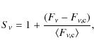
|
(1) |
where
For this work, the continuum was consistently chosen for all sources by
fitting a third-order polynomial to data between 5.0 and 7.5 ![]() m and between 13.0 and 16.0
m and between 13.0 and 16.0 ![]() m (cf. Furlan et al. 2006). The regular continuum was used rather than the frequency-averaged continuum, resulting in the peak strength
m (cf. Furlan et al. 2006). The regular continuum was used rather than the frequency-averaged continuum, resulting in the peak strength
![]() and the shape F11.3/F9.8. This does not change the results significantly (see Kessler-Silacci et al. 2006).
and the shape F11.3/F9.8. This does not change the results significantly (see Kessler-Silacci et al. 2006).
The results are listed in Table 4 and shown in Fig. 2. The upper panel of Fig. 2 gives (
![]() )/
)/
![]() vs.
vs.
![]() ,
showing a clear correlation between the two definitions of the strength of the 10-
,
showing a clear correlation between the two definitions of the strength of the 10-![]() m feature. The lower panel gives
m feature. The lower panel gives
![]() vs.
F11.3/F9.8, also showing a correlation, confirming the results of Kessler-Silacci et al. (2006).
This figure also confirms that our sample covers a large range in
silicate-feature characteristics. It follows that the three
methods to quantify the strength or shape of the 10-
vs.
F11.3/F9.8, also showing a correlation, confirming the results of Kessler-Silacci et al. (2006).
This figure also confirms that our sample covers a large range in
silicate-feature characteristics. It follows that the three
methods to quantify the strength or shape of the 10-![]() m feature give completely consistent results. When comparing the 10-
m feature give completely consistent results. When comparing the 10-![]() m
feature with the mm slope in Sect. 5 below, the strength defined as (
m
feature with the mm slope in Sect. 5 below, the strength defined as (
![]() )/
)/
![]() will be used. The source that lies towards the top and to the right of
the general trend in the lower panel is RX J1615.3-3255, an
isolated source slightly to the north of the Lupus star-forming clouds.
will be used. The source that lies towards the top and to the right of
the general trend in the lower panel is RX J1615.3-3255, an
isolated source slightly to the north of the Lupus star-forming clouds.
![\begin{figure}
\par\includegraphics[width=8.5cm,clip]{13150fi2.eps}
\end{figure}](/articles/aa/full_html/2010/07/aa13150-09/img95.png)
|
Figure 2:
Upper panel: the peak strength of the 10- |
| Open with DEXTER | |
3.4 10-m feature vs. mm slope
Figures 3 and 4 show the mm slope ![]() ,
measured between 1 and 3 mm, as a function of the strength of the 10-
,
measured between 1 and 3 mm, as a function of the strength of the 10-![]() m feature
m feature
![]() .
Only the slope between 1 and 3 mm is used, to make the
sample as consistent as possible. However, as noted before,
the slope between 3 and 7 mm is consistent with that
between 1 and 3 mm for most sources. Included are the
sources from this study, as well as eleven sources located in the
Taurus-Auriga star-forming region discussed in Rodmann et al. (2006) and
Andrews & Williams (2007) for which the
spectral slope between 1 and 3 mm could be determined, and
the sources located in Lupus and Chamaeleon discussed in Lommen et al. (2007). The total number of sources used is 31; the complete list is given in Table 5. In Fig. 4,
the sources are sorted by their star-forming region. The smaller
symbols designate single stars and the larger symbols binaries
(or stars that are members of a multiple system). The open
symbol to the left is T Cha, an evolved system that does not
show any silicate emission and is not used in the analysis, and the
open symbol in the centre designates the ``cold disc'' CS Cha.
.
Only the slope between 1 and 3 mm is used, to make the
sample as consistent as possible. However, as noted before,
the slope between 3 and 7 mm is consistent with that
between 1 and 3 mm for most sources. Included are the
sources from this study, as well as eleven sources located in the
Taurus-Auriga star-forming region discussed in Rodmann et al. (2006) and
Andrews & Williams (2007) for which the
spectral slope between 1 and 3 mm could be determined, and
the sources located in Lupus and Chamaeleon discussed in Lommen et al. (2007). The total number of sources used is 31; the complete list is given in Table 5. In Fig. 4,
the sources are sorted by their star-forming region. The smaller
symbols designate single stars and the larger symbols binaries
(or stars that are members of a multiple system). The open
symbol to the left is T Cha, an evolved system that does not
show any silicate emission and is not used in the analysis, and the
open symbol in the centre designates the ``cold disc'' CS Cha.
Table 5: List of sources used in the analysis.
![\begin{figure}
\par\includegraphics[width=8.8cm,clip]{13150fi3.eps}
\end{figure}](/articles/aa/full_html/2010/07/aa13150-09/img96.png)
|
Figure 3:
The mm slope as measured between 1 and 3 mm as a function of the strength of the 10- |
| Open with DEXTER | |
![\begin{figure}
\par\includegraphics[width=8.8cm,clip]{13150fi4.eps}
\end{figure}](/articles/aa/full_html/2010/07/aa13150-09/img97.png)
|
Figure 4:
Same as Fig. 3, with the different sources sorted by star-forming region: filled circles: Lupus, five-pointed stars: Chamaeleon, cross: Corona Australis, diamonds: Taurus-Auriga, and squares:
Serpens. The ellipses show the concentrations of sources located in the
Taurus-Auriga star-forming region (lower left),
the Chamaeleon I cloud (top centre), and the Lupus 1 and
Lupus 2 clouds (upper left). The remaining two Lupus sources in
the upper right are an isolated source (RX J1615-.3-3255,
right-most dot) and a source from the Lupus 3 cloud (RY Lup,
upper-most dot). The small symbols designate the single stars and the
large symbols designate multiple systems. The open five-pointed star to
the left is for T Cha, an evolved cold disc which shows no
silicate emission around 10 |
| Open with DEXTER | |
The sources in the sample shown in Fig. 3 lie in a broad band roughly running from the lower left (shallow mm slope and weak 10-![]() m feature) to the upper right (steep mm slope and strong 10-
m feature) to the upper right (steep mm slope and strong 10-![]() m
feature). The sole exception is the source RY Tau, which lies
in the lower right corner. The mm slope and the strength of
the 10-
m
feature). The sole exception is the source RY Tau, which lies
in the lower right corner. The mm slope and the strength of
the 10-![]() m
feature correlate weakly for the full sample: the Spearman rank
correlation coefficient is 0.50, with a 99.5% confidence
level. However, if the point for RY Tau is excluded,
the Spearman rank coefficient becomes 0.66, with
a 99.99% confidence level. Note that RY Tau is a
peculiar source: it is found to be a rapidly rotating UX Or-type
star powering a microjet (e.g., Petrov et al. 1999; Agra-Amboage et al. 2009). A possible explanation for its location in the 10-
m
feature correlate weakly for the full sample: the Spearman rank
correlation coefficient is 0.50, with a 99.5% confidence
level. However, if the point for RY Tau is excluded,
the Spearman rank coefficient becomes 0.66, with
a 99.99% confidence level. Note that RY Tau is a
peculiar source: it is found to be a rapidly rotating UX Or-type
star powering a microjet (e.g., Petrov et al. 1999; Agra-Amboage et al. 2009). A possible explanation for its location in the 10-![]() m-feature
vs mm-slope diagram is a rather evolved disc in which a recent
collision event produced small grains. This may be similar to the
effect recently observed in EX Lup, in which a significantly
more crystalline 10-
m-feature
vs mm-slope diagram is a rather evolved disc in which a recent
collision event produced small grains. This may be similar to the
effect recently observed in EX Lup, in which a significantly
more crystalline 10-![]() m feature was observed after an outburst (Ábrahám et al. 2009). RY Tau will not be included in the further discussion.
m feature was observed after an outburst (Ábrahám et al. 2009). RY Tau will not be included in the further discussion.
Figure 4 suggests a grouping in the ![]() m-vs.-mm diagram
according to parental cloud, with the sources from the Taurus-Auriga
star-forming region more concentrated in the lower left, the Lupus
sources more to the upper left, and the Chamaeleon sources more to the
centre right. Note that the six Lupus sources that are on the left part
of the diagram (from top to bottom: IM Lup, Sz 66,
Sz 65, RU Lup, GW Lup, and HT Lup) are all located
in the Lupus 1 and Lupus 2 clouds, whereas the remaining two
Lupus sources are located in Lupus 3 (top-most source,
RY Lup) and off-cloud (RX J1615.3-3255). Larger-number
statistics are needed to confirm this grouping by star-forming region
in the
m-vs.-mm diagram
according to parental cloud, with the sources from the Taurus-Auriga
star-forming region more concentrated in the lower left, the Lupus
sources more to the upper left, and the Chamaeleon sources more to the
centre right. Note that the six Lupus sources that are on the left part
of the diagram (from top to bottom: IM Lup, Sz 66,
Sz 65, RU Lup, GW Lup, and HT Lup) are all located
in the Lupus 1 and Lupus 2 clouds, whereas the remaining two
Lupus sources are located in Lupus 3 (top-most source,
RY Lup) and off-cloud (RX J1615.3-3255). Larger-number
statistics are needed to confirm this grouping by star-forming region
in the ![]() m-vs.-mm diagram.
m-vs.-mm diagram.
Kessler-Silacci et al. (2006) found a correlation between the spectral type of a source and the strength and shape of the 10-![]() m
silicate feature, brown dwarfs having predominantly flatter and
Herbig-Ae/Be stars having more peaked features. It was found
that this is most likely due to the location of the silicate emission
region: Kessler-Silacci et al. (2007) showed that the radius of the 10-
m
silicate feature, brown dwarfs having predominantly flatter and
Herbig-Ae/Be stars having more peaked features. It was found
that this is most likely due to the location of the silicate emission
region: Kessler-Silacci et al. (2007) showed that the radius of the 10-![]() m silicate emission zone in the disc goes roughly as
m silicate emission zone in the disc goes roughly as
![]() .
Hence, the 10-
.
Hence, the 10-![]() m
feature probes a radius further from the star for early-type stars than
for late-type stars. In this context it is interesting to see whether a
correlation with spectral type is found in the 10-
m
feature probes a radius further from the star for early-type stars than
for late-type stars. In this context it is interesting to see whether a
correlation with spectral type is found in the 10-![]() m-feature vs. mm-slope diagram (Fig. 5).
The M stars in the sample presented here are concentrated to the
left, the F and G stars to the lower left, and the
K stars are found both in the lower left and in the upper right.
Hence, no clear correlation with spectral type is found here.
It is interesting to note, though, that the F and
G sources RY Tau and RY Lup show up isolated from the
other F and G sources. This may indicate that these sources
are indeed different from the other sources in the sample, justifying
the choice not to include RY Tau in the analysis.
m-feature vs. mm-slope diagram (Fig. 5).
The M stars in the sample presented here are concentrated to the
left, the F and G stars to the lower left, and the
K stars are found both in the lower left and in the upper right.
Hence, no clear correlation with spectral type is found here.
It is interesting to note, though, that the F and
G sources RY Tau and RY Lup show up isolated from the
other F and G sources. This may indicate that these sources
are indeed different from the other sources in the sample, justifying
the choice not to include RY Tau in the analysis.
![\begin{figure}
\par\includegraphics[width=8.5cm,clip]{13150fi5.eps}
\end{figure}](/articles/aa/full_html/2010/07/aa13150-09/img99.png)
|
Figure 5: Same as Fig. 3, with the different sources sorted by spectral type: orange: F and G, blue: K, and green: M. |
| Open with DEXTER | |
4 Modelling
4.1 Disk model parameters and SEDs
Variations in the strength and shape of the 10-![]() m feature (e.g., Kessler-Silacci et al. 2006) as well as in the (sub)mm slope (e.g., Beckwith et al. 1990)
can be explained by variations in the dominating grain size in the
circumstellar discs, so that one may expect a correlation between
properties of the 10-
m feature (e.g., Kessler-Silacci et al. 2006) as well as in the (sub)mm slope (e.g., Beckwith et al. 1990)
can be explained by variations in the dominating grain size in the
circumstellar discs, so that one may expect a correlation between
properties of the 10-![]() m
feature and the mm slope. Such a correlation is found
for the sample as a whole (see previous section) and this may
imply that grain growth occurs in the whole disc simultaneously, or
that grains grow in the inner disc and the new grain size distribution
is very efficiently spread to the outer disc through radial mixing.
Both processes will have the effect of a shift of dust mass from small
particles to larger grains. To study this more quantitatively, we
ran a number of models with varying grain size distributions.
m
feature and the mm slope. Such a correlation is found
for the sample as a whole (see previous section) and this may
imply that grain growth occurs in the whole disc simultaneously, or
that grains grow in the inner disc and the new grain size distribution
is very efficiently spread to the outer disc through radial mixing.
Both processes will have the effect of a shift of dust mass from small
particles to larger grains. To study this more quantitatively, we
ran a number of models with varying grain size distributions.
We use the axisymmetric radiative-transfer code RADMC, developed by Dullemond (2002) and
Dullemond & Dominik (2004). The model
consists of a flaring disc, heated passively by radiation from the
central star, and includes a hot inner wall, which is directly
irradiated by the central star (Natta et al. 2001; see also Dullemond et al. 2001). The surface density of the disc as a function of radius ![]() is defined to be:
is defined to be:
with n = -1. The total gas+dust disc mass was fixed to
For the dust opacities, we use a mixture of 80% amorphous
olivine and 20% armorphous carbon (percentages by mass). The
opacities are calculated using a Distribution of Hollow Spheres (DHS,
see Min et al. 2003). The total volume of the spheres occupied by the inclusion f is taken in the range
f = [0, 0.8]. It was found (e.g. Dullemond & Dominik 2004; D'Alessio et al. 2001; Chiang et al. 2001)
that the mm slope changes if one goes from a disc with only
``small'' particles to a disc that also contains some ``large'' grains.
Dullemond & Dominik started with a disc in which the
dust is made up of only 0.1-![]() m-sized
particles and subsequently replaced 90%, 99%, 99.9%, 99.99%,
and 99.999% of the dust by large, 2-mm-sized grains. The
mm slope changes considerably when the mass fraction in large
grains is changed from 0 to 90%, but it does not change
further if a larger fraction of the dust mass is put in large grains
(see Fig. 7 in Dullemond & Dominik 2004).
This is a result of the fact that at 1 mm the opacity is dominated
by the large grains, virtually independent of the mass fraction
(K. Pontoppidan, priv. comm.). Although it is possible that a more
gradual change in the mm slope is seen when smaller mass fractions
are put in large grains, it does seem to be more important what
the largest grain size is, rather than which fraction of the dust is
contained in such large grains. We therefore chose not to use a bimodal
dust distribution, but a distribution in which the size of the grains
ranges from a minimum value
m-sized
particles and subsequently replaced 90%, 99%, 99.9%, 99.99%,
and 99.999% of the dust by large, 2-mm-sized grains. The
mm slope changes considerably when the mass fraction in large
grains is changed from 0 to 90%, but it does not change
further if a larger fraction of the dust mass is put in large grains
(see Fig. 7 in Dullemond & Dominik 2004).
This is a result of the fact that at 1 mm the opacity is dominated
by the large grains, virtually independent of the mass fraction
(K. Pontoppidan, priv. comm.). Although it is possible that a more
gradual change in the mm slope is seen when smaller mass fractions
are put in large grains, it does seem to be more important what
the largest grain size is, rather than which fraction of the dust is
contained in such large grains. We therefore chose not to use a bimodal
dust distribution, but a distribution in which the size of the grains
ranges from a minimum value
![]() to a maximum value
to a maximum value
![]() according to
according to
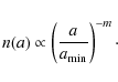
|
(3) |
This power-law distribution is expected on theoretical grounds whenever grain-grain collisions lead to shattering (Dohnanyi 1969). It should be noted that models which include grain growth may lead to different grain size distributions (e.g., Tanaka et al. 2005; Dullemond & Dominik 2005). The value
Table 6: Model parameters.
The resulting SEDs from six models, with
![]() varying and the other parameters kept fixed, is shown in Fig. 6. In these models,
varying and the other parameters kept fixed, is shown in Fig. 6. In these models,
![]() was
fixed to 300 AU and the scale height was kept fixed at the same
value in all models to show only the effect of varying
was
fixed to 300 AU and the scale height was kept fixed at the same
value in all models to show only the effect of varying
![]() .
Strong variations are seen in all wavelength regimes, from the near-infrared through the mm. At wavelengths
.
Strong variations are seen in all wavelength regimes, from the near-infrared through the mm. At wavelengths
![]()
![]() m, grain size distributions without grains larger than 1
m, grain size distributions without grains larger than 1 ![]() m
give such a high opacity that the central star is significantly
reddened. In the mid- and far infrared, the flux drops with
increasing maximum grain size. The (sub)mm part of the SED does
not
change appreciably unless grains with sizes of
m
give such a high opacity that the central star is significantly
reddened. In the mid- and far infrared, the flux drops with
increasing maximum grain size. The (sub)mm part of the SED does
not
change appreciably unless grains with sizes of ![]() 100
100 ![]() m or larger are included. After that, the (sub)mm slope becomes shallower quite rapidly with increasing
m or larger are included. After that, the (sub)mm slope becomes shallower quite rapidly with increasing
![]() .
This figure also demonstrates that care must be taken when estimating
the disc mass from the (sub)mm emission alone: even when the dust
composition is kept the same, assuming a different grain size
distribution may already change the opacity at 1 mm by an
order of magnitude, which will give an equally large uncertainty in the
mass estimate from an observed flux at that wavelength.
.
This figure also demonstrates that care must be taken when estimating
the disc mass from the (sub)mm emission alone: even when the dust
composition is kept the same, assuming a different grain size
distribution may already change the opacity at 1 mm by an
order of magnitude, which will give an equally large uncertainty in the
mass estimate from an observed flux at that wavelength.
![\begin{figure}
\par\includegraphics[width=8.5cm,clip]{13150fi6.eps}
\end{figure}](/articles/aa/full_html/2010/07/aa13150-09/img121.png)
|
Figure 6:
Spectral energy distributions (SEDs) for models of a 5 |
| Open with DEXTER | |
4.2 10-m feature vs. mm slope
In Fig. 7, we plot the strength of the 10-![]() m feature vs. the mm slope for different models. The strength of the 10-
m feature vs. the mm slope for different models. The strength of the 10-![]() m feature
m feature
![]() is defined as in Furlan et al. (2006) and the mm slope
is defined as in Furlan et al. (2006) and the mm slope ![]() is determined between 1.0 and 3.0 mm. The main aim of this figure is to show the variation of the 10-
is determined between 1.0 and 3.0 mm. The main aim of this figure is to show the variation of the 10-![]() m-feature
strength and mm slope with various parameters. While the
quantitative details will depend on the specific dust and disc
parameters used, the qualitative trends found in these figures should
be robust.
m-feature
strength and mm slope with various parameters. While the
quantitative details will depend on the specific dust and disc
parameters used, the qualitative trends found in these figures should
be robust.
In each of the panels, the results for different maximum grain
sizes are shown. The size of the triangles is an indication for the
maximum grain size under consideration. A general trend is
observed, in the sense that the models with only small grains end
up in the upper right corner of the micron-vs.-mm diagram (strong 10-![]() m
feature and steep mm slope), the models which include grains of mm
sizes or larger end up more to the lower left of the diagram (weak 10-
m
feature and steep mm slope), the models which include grains of mm
sizes or larger end up more to the lower left of the diagram (weak 10-![]() m feature and shallower mm slope), and those with grain sizes of up to 10 or 100
m feature and shallower mm slope), and those with grain sizes of up to 10 or 100 ![]() m end up towards the upper left corner of the diagram (weak 10-
m end up towards the upper left corner of the diagram (weak 10-![]() m
feature and steep mm slope). A possible evolutionary
sequence, in which the maximum grain size in the disc gradually
increases, is indicated by the arrows: first, the 10-
m
feature and steep mm slope). A possible evolutionary
sequence, in which the maximum grain size in the disc gradually
increases, is indicated by the arrows: first, the 10-![]() m feature becomes weaker and later, the mm slope becomes shallower. A test to check whether radial variation of
m feature becomes weaker and later, the mm slope becomes shallower. A test to check whether radial variation of
![]() - larger grains closer to the star, where the densities are higher - did not show any significant difference.
- larger grains closer to the star, where the densities are higher - did not show any significant difference.
The models show the effect of the temperature and luminosity of the central star on the strength of the 10-![]() m feature and the steepness of the mm slope. The left column shows the results for a central star with
m feature and the steepness of the mm slope. The left column shows the results for a central star with
![]() K and
K and
![]() and the right column for
and the right column for
![]() K and
K and
![]() .
In Figs. 7a and b, the power-law slope of the grain size distribution is varied from m = 2.5 to 3.0, 3.5, and 4.0. It appears that only grain size distributions with m = 2.5 produce completely flat 10-
.
In Figs. 7a and b, the power-law slope of the grain size distribution is varied from m = 2.5 to 3.0, 3.5, and 4.0. It appears that only grain size distributions with m = 2.5 produce completely flat 10-![]() m silicate features as well as mm slopes with
m silicate features as well as mm slopes with
![]() ,
whereas grain size distributions with m = 4.0 never produce a mm slope with
,
whereas grain size distributions with m = 4.0 never produce a mm slope with
![]() .
Furthermore, the strongest 10-
.
Furthermore, the strongest 10-![]() m features are only obtained with a central star of 4000 K and
m features are only obtained with a central star of 4000 K and
![]() .
.
![\begin{figure}
\par\includegraphics[width=17cm,clip]{13150fi7.eps}
\end{figure}](/articles/aa/full_html/2010/07/aa13150-09/img126.png)
|
Figure 7:
The mm slope |
| Open with DEXTER | |
In Figs. 7c and d, the power-law slope of the grain size distribution is fixed to m = 3.5. The disc radius
![]() is varied between 100, 200, and 300 AU. This has a small effect on the strength of the 10-
is varied between 100, 200, and 300 AU. This has a small effect on the strength of the 10-![]() m feature, particularly for
m feature, particularly for
![]() K and
K and
![]()
![]() m.
This can be understood in the sense that for a smaller disc with the
same dust mass, a larger amount of mass is closer to the star and
thus radiates in the infrared. The mm slope of the SED is practically
unaffected.
m.
This can be understood in the sense that for a smaller disc with the
same dust mass, a larger amount of mass is closer to the star and
thus radiates in the infrared. The mm slope of the SED is practically
unaffected.
Figures 7e and f show the results for models in which the power-law slope of the grain size distribution was fixed to m = 3.5, the disc outer radius to
![]() AU, and for which the inclination i
under which the disc is observed is varied. In most cases,
the inclination has a limited effect on both the strength of the
10-
AU, and for which the inclination i
under which the disc is observed is varied. In most cases,
the inclination has a limited effect on both the strength of the
10-![]() m feature and the mm slope of the SED. Only under very high inclination (e.g., 75
m feature and the mm slope of the SED. Only under very high inclination (e.g., 75![]() ,
where 90
,
where 90![]() is edge-on) does the 10-
is edge-on) does the 10-![]() m
feature appear in absorption (not shown). A similar effect is
seen if the discs are more flaring than found in vertical hydrostatic
equilibrium: the 10-
m
feature appear in absorption (not shown). A similar effect is
seen if the discs are more flaring than found in vertical hydrostatic
equilibrium: the 10-![]() m feature is primarily weakened, because of the enhanced extinction under most inclinations.
m feature is primarily weakened, because of the enhanced extinction under most inclinations.
A second set of models is run to investigate the effects of dust
settling, i.e., the process in which larger grains fall to the
disc midplane under the influence of gravity, while the smaller grains
stay suspended in the disc atmosphere. As mentioned before, Dullemond & Dominik (2008) found that a bimodal grain size distribution can explain variations in the strength of the 10-![]() m feature,
but only under specific circumstances. They looked at grains that are mainly responsible for the 10-
m feature,
but only under specific circumstances. They looked at grains that are mainly responsible for the 10-![]() m feature, in particular grains of 3
m feature, in particular grains of 3 ![]() m and of
m and of ![]() 1
1 ![]() m.
To study the effect of the settling of larger grains, we ran a
number of models with up to six different grain size distributions:
grains with sizes between 0.003 and 0.1
m.
To study the effect of the settling of larger grains, we ran a
number of models with up to six different grain size distributions:
grains with sizes between 0.003 and 0.1 ![]() m, between 0.1 and 1
m, between 0.1 and 1 ![]() m, 1 and 10, 10 and 100, 100 and 1000, and finally between 1000 and 10 000
m, 1 and 10, 10 and 100, 100 and 1000, and finally between 1000 and 10 000 ![]() m. The degree of settling is given by a parameter s,
varying between 0.25, 0.50, 0.75, and 1.00, and is chosen to
be different for each of the grain size distributions: the larger
the grains, the larger the degree of settling. For example,
if H denotes the self-consistent scale height, a settling parameter s = 0.75 indicates that:
m. The degree of settling is given by a parameter s,
varying between 0.25, 0.50, 0.75, and 1.00, and is chosen to
be different for each of the grain size distributions: the larger
the grains, the larger the degree of settling. For example,
if H denotes the self-consistent scale height, a settling parameter s = 0.75 indicates that:
- grains between 0.003 and 0.1
- grains between 0.1 and 1 m are at
 ;
;
- grains between 1 and 10 m are at
 ;
;
- grains between 10 and 100 m are at
 ;
;
- grains between 100 and 1000 m are at
 ;
;
- grains between 1000 and 10 000 m are at
 .
.
These models are run using the radiative transfer code MCMax (Min et al. 2009). MCMax and RADMC were benchmarked against the results of Pascucci et al. (2004) and the differences in the resulting SEDs are minimal, with in particular the 10-![]() m features being practically indistinguishable (see the Appendix in Min et al. 2009). The results for the settling are shown in Fig. 8. Note that the strength of the 10-
m features being practically indistinguishable (see the Appendix in Min et al. 2009). The results for the settling are shown in Fig. 8. Note that the strength of the 10-![]() m feature increases when settling is switched on, but does not increase significantly more when the value of s
is decreased more (i.e., when the degree of settling is
increased). The slope in the mm part of the SED is practically
unaffected by the degree of settling.
m feature increases when settling is switched on, but does not increase significantly more when the value of s
is decreased more (i.e., when the degree of settling is
increased). The slope in the mm part of the SED is practically
unaffected by the degree of settling.
![\begin{figure}
\par\includegraphics[width=8.5cm,clip]{13150fi8.eps}
\end{figure}](/articles/aa/full_html/2010/07/aa13150-09/img134.png)
|
Figure 8:
Strength of the 10- |
| Open with DEXTER | |
It can be concluded that a variation of the maximum grain size
![]() affects both the strength of the 10-
affects both the strength of the 10-![]() m feature and the steepness of the mm slope
m feature and the steepness of the mm slope ![]() :
a larger maximum grain size yields a weaker 10-
:
a larger maximum grain size yields a weaker 10-![]() m feature and a shallower mm slope. This effect is robust against variations in the degree of settling s, which only affects the strength of the 10-
m feature and a shallower mm slope. This effect is robust against variations in the degree of settling s, which only affects the strength of the 10-![]() m feature. Only varying the maximum grain size is, however, not enough to explain the range in 10-
m feature. Only varying the maximum grain size is, however, not enough to explain the range in 10-![]() m
features and mm slopes that is observed. Variations in the power-law
index of the grain size distribution and the temperature and luminosity
of the central source are required as well to cover the full observed
range. For example, only models with a central-star temperature of
at least 4000 K yield a 10-
m
features and mm slopes that is observed. Variations in the power-law
index of the grain size distribution and the temperature and luminosity
of the central source are required as well to cover the full observed
range. For example, only models with a central-star temperature of
at least 4000 K yield a 10-![]() m feature with a strength of
m feature with a strength of
![]() ;
models with relatively flat or shallow grain size distributions are required to get mm slopes of
;
models with relatively flat or shallow grain size distributions are required to get mm slopes of
![]() (see also Ricci et al. 2010; Natta et al. 2007).
(see also Ricci et al. 2010; Natta et al. 2007).
5 Discussion
A correlation between the strength of the 10-![]() m
silicate feature and the slope between 1 and 3 mm is observed
in a sample of in total 31 T-Tauri stars. This seems to imply
that, while in the upper layers of the hot inner disc small grains are
still coagulating to a few microns in size,
in the cold mid-plane of the outer disc large grains of at least
several millimetres in size are already being formed. One should keep
in mind, though, that the 10-
m
silicate feature and the slope between 1 and 3 mm is observed
in a sample of in total 31 T-Tauri stars. This seems to imply
that, while in the upper layers of the hot inner disc small grains are
still coagulating to a few microns in size,
in the cold mid-plane of the outer disc large grains of at least
several millimetres in size are already being formed. One should keep
in mind, though, that the 10-![]() m
silicate feature only probes the hot surface layers of the inner disc.
It is therefore possible, and even likely, that large grains or
boulders exist in the mid-plane of the inner disc. The tentative
correlation seen in our observations show, however, that the inner and
outer discs of young stellar objects do not evolve independently from
each other. Furthermore, the gradual decline of the 10-
m
silicate feature only probes the hot surface layers of the inner disc.
It is therefore possible, and even likely, that large grains or
boulders exist in the mid-plane of the inner disc. The tentative
correlation seen in our observations show, however, that the inner and
outer discs of young stellar objects do not evolve independently from
each other. Furthermore, the gradual decline of the 10-![]() m
feature as the mm slope becomes shallower implies that micron-sized
grains remain present in the disc atmosphere as cm-sized pebbles are
already forming in the mid-plane.
m
feature as the mm slope becomes shallower implies that micron-sized
grains remain present in the disc atmosphere as cm-sized pebbles are
already forming in the mid-plane.
The radiative-transfer programmes RADMC and MCMax were used to
run a number of models with varying disc parameters, stellar
parameters, and power-law grain size distributions. The only parameter
that affects the strength of the 10-![]() m feature and the mm slope of the SED simultaneously is the maximum grain size
m feature and the mm slope of the SED simultaneously is the maximum grain size
![]() :
a larger
:
a larger
![]() gives both a weaker 10-
gives both a weaker 10-![]() m
feature and a shallower mm slope. This result is very robust
against variations of the other parameters. There are, however,
a few striking results when the models are compared to the
observations. Firstly, the strongest 10-
m
feature and a shallower mm slope. This result is very robust
against variations of the other parameters. There are, however,
a few striking results when the models are compared to the
observations. Firstly, the strongest 10-![]() m silicate features, with
m silicate features, with
![]() ,
can only be reproduced for a star with
,
can only be reproduced for a star with
![]() K and
K and
![]() ,
whereas a tempearature of 3000 K and a luminosity of 1
,
whereas a tempearature of 3000 K and a luminosity of 1 ![]() seem to be more common for observed T-Tauri stars (see Evans et al. 2009).
This may in part be a selection effect: the sources with the
hottest central stars are the most likely to have strong mm fluxes,
making it more likely for them to provide a good mm slope.
A subsample of the sources of Evans et al. (2009) which had enough data points in the SED to provide a decent model fit also gave on average a higher
seem to be more common for observed T-Tauri stars (see Evans et al. 2009).
This may in part be a selection effect: the sources with the
hottest central stars are the most likely to have strong mm fluxes,
making it more likely for them to provide a good mm slope.
A subsample of the sources of Evans et al. (2009) which had enough data points in the SED to provide a decent model fit also gave on average a higher
![]() than would be expected from the near-infrared colours alone
(B. Merín, priv. comm.). The physical reason for the increase
in strength of the 10-
than would be expected from the near-infrared colours alone
(B. Merín, priv. comm.). The physical reason for the increase
in strength of the 10-![]() m
feature with temperature lies in the fact that the photosphere is still
an important continuum source. When the temperature of the star is
increased, the relative contribution from the photosphere becomes
smaller and the peak/continuum ratio of the feature goes up.
m
feature with temperature lies in the fact that the photosphere is still
an important continuum source. When the temperature of the star is
increased, the relative contribution from the photosphere becomes
smaller and the peak/continuum ratio of the feature goes up.
Secondly, the sources with
![]() as well as those with a mm slope
as well as those with a mm slope
![]() can only be reproduced if the power-law slope of the grain size distribution is as low as m = 2.5. A slope m = 4.0 does not allow the mm slope to get below 3.0. The strength of the 10-
can only be reproduced if the power-law slope of the grain size distribution is as low as m = 2.5. A slope m = 4.0 does not allow the mm slope to get below 3.0. The strength of the 10-![]() m feature remains at least as large as 1.4, and even 1.6 in the case
m feature remains at least as large as 1.4, and even 1.6 in the case
![]() K.
This appears to indicate that, as grains are growing to mm and cm
sizes, the power-law slope of the grain size distribution becomes
shallower. It is, however, more likely that a power-law grain size
distribution with a mimimum grain size of
K.
This appears to indicate that, as grains are growing to mm and cm
sizes, the power-law slope of the grain size distribution becomes
shallower. It is, however, more likely that a power-law grain size
distribution with a mimimum grain size of
![]()
![]() m no longer applies. Either the effective minimum grain size increases, as suggested by the work of Olofsson et al. (2009),
or a different grain size distribution is more applicable,
such as naturally obtained from models including fragmentation
(e.g., Dullemond & Dominik 2005).
m no longer applies. Either the effective minimum grain size increases, as suggested by the work of Olofsson et al. (2009),
or a different grain size distribution is more applicable,
such as naturally obtained from models including fragmentation
(e.g., Dullemond & Dominik 2005).
It is important at this point to note once more that the 10-![]() m
feature originates entirely from the disc atmosphere; (sub)micron-sized
dust grains that are closer to the midplane are not observable due to
the optical thickness of the infrared emission. The emission at
(sub)mm wavelengths, on the other hand, is predominantly
optically thin; hence, it may originate from the whole disc.
In fact, the bulk of the (sub)mm emission comes from the
midplane, since the larger grains will settle to the midplane.
To study the effect of the settling of larger (mm and
cm-sized) grains, we ran a number of models with up to six different
grain size distributions. The smallest grains (
0.003 < a < 0.1
m
feature originates entirely from the disc atmosphere; (sub)micron-sized
dust grains that are closer to the midplane are not observable due to
the optical thickness of the infrared emission. The emission at
(sub)mm wavelengths, on the other hand, is predominantly
optically thin; hence, it may originate from the whole disc.
In fact, the bulk of the (sub)mm emission comes from the
midplane, since the larger grains will settle to the midplane.
To study the effect of the settling of larger (mm and
cm-sized) grains, we ran a number of models with up to six different
grain size distributions. The smallest grains (
0.003 < a < 0.1 ![]() m)
followed the gas, while the increasingly larger grains were located
increasingly closer to the midplane. It turns out that the
strength of the 10-
m)
followed the gas, while the increasingly larger grains were located
increasingly closer to the midplane. It turns out that the
strength of the 10-![]() m
feature always increases when settling is switched on,
but does not increase significantly more when the value of the
settling parameter s
is decreased more (i.e., when the degree of settling is
increased). This can be understood from the fact that a small degree of
settling already removes
the larger grains from the disc atmosphere. Since the 10-
m
feature always increases when settling is switched on,
but does not increase significantly more when the value of the
settling parameter s
is decreased more (i.e., when the degree of settling is
increased). This can be understood from the fact that a small degree of
settling already removes
the larger grains from the disc atmosphere. Since the 10-![]() m
feature originates in the disc atmosphere, it does not matter
where the larger grains reside, as long as they are not too close
to the surface. The slope in the mm part of the SED is practically
unaffected by the degree of settling. This is because the disc is
optically thin at these long wavelengths and hence it does
not matter where in the disc the large grains, which determine the
brightness at long wavelengths, are located. While the absolute
strength and slope depend on the detailed dust and disc model
parameters, the trends found here should be robust. Further
modelling and exploration of the large parameter space are left to a
future paper.
m
feature originates in the disc atmosphere, it does not matter
where the larger grains reside, as long as they are not too close
to the surface. The slope in the mm part of the SED is practically
unaffected by the degree of settling. This is because the disc is
optically thin at these long wavelengths and hence it does
not matter where in the disc the large grains, which determine the
brightness at long wavelengths, are located. While the absolute
strength and slope depend on the detailed dust and disc model
parameters, the trends found here should be robust. Further
modelling and exploration of the large parameter space are left to a
future paper.
The observations indicate a clustering of the sources per
star-forming region. The T-Tauri stars in Chamaeleon show the strongest
10-![]() m
features, as well as the steepest mm slopes. The T-Tauri stars located
in the Lupus 1 and Lupus 2 clouds have somewhat weaker 10-
m
features, as well as the steepest mm slopes. The T-Tauri stars located
in the Lupus 1 and Lupus 2 clouds have somewhat weaker 10-![]() m
features and mm slopes that are a bit shallower than the Chamaelon
sources. The sources located in the Taurus-Auriga star-forming region,
finally, have the weakest 10-
m
features and mm slopes that are a bit shallower than the Chamaelon
sources. The sources located in the Taurus-Auriga star-forming region,
finally, have the weakest 10-![]() m
features and the shallowest mm slope. Although the number statistics
are too low to draw strong conclusions from this grouping per
star-forming region, it is intersesting to hypothesise as to what
might be the origin of this grouping. It could in principle be due
to a selection effect. To check for this, the strengths of
the 10-
m
features and the shallowest mm slope. Although the number statistics
are too low to draw strong conclusions from this grouping per
star-forming region, it is intersesting to hypothesise as to what
might be the origin of this grouping. It could in principle be due
to a selection effect. To check for this, the strengths of
the 10-![]() m features of the eleven sources from Furlan et al. (2006)
included in this work were compared with those of the 72 Taurus
sources not included in this work and the two samples were found to be
statistically indistinguishable. Furthermore, after this paper was
submitted, Ricci et al. (2010) published mm slopes for a total of 21 sources in the Taurus-Auriga star-forming region. Ricci et al. found the slopes between 1 and 3 mm all to be
m features of the eleven sources from Furlan et al. (2006)
included in this work were compared with those of the 72 Taurus
sources not included in this work and the two samples were found to be
statistically indistinguishable. Furthermore, after this paper was
submitted, Ricci et al. (2010) published mm slopes for a total of 21 sources in the Taurus-Auriga star-forming region. Ricci et al. found the slopes between 1 and 3 mm all to be
![]() ;
the corresponding strengths of the 10-
;
the corresponding strengths of the 10-![]() m features are
m features are
![]() for 17 of those 21 sources (Furlan et al. 2006). Thus, these sources mainly populate the lower left corner of the
for 17 of those 21 sources (Furlan et al. 2006). Thus, these sources mainly populate the lower left corner of the ![]() m-vs.-mm diagram.
It is then tempting to attribute the clustering to an evolutionary
sequence, with the Chamaeleon sources being the least evolved and the
Taurus-Auriga sources the most evolved. If the evolution proceeds
equally fast in each star-forming region, Taurus-Auriga would then be
the oldest star-forming region and Chamaeleon the youngest. However,
ages of pre-main-sequence stars are notoriously difficult to determine
and there is a large spread of stellar ages within each region
(see Table 1).
Note that a chemical differentiation, with, e.g., Chamaeleon a region
with more silicates than Taurus, would mainly have an effect on the
strength of the 10-
m-vs.-mm diagram.
It is then tempting to attribute the clustering to an evolutionary
sequence, with the Chamaeleon sources being the least evolved and the
Taurus-Auriga sources the most evolved. If the evolution proceeds
equally fast in each star-forming region, Taurus-Auriga would then be
the oldest star-forming region and Chamaeleon the youngest. However,
ages of pre-main-sequence stars are notoriously difficult to determine
and there is a large spread of stellar ages within each region
(see Table 1).
Note that a chemical differentiation, with, e.g., Chamaeleon a region
with more silicates than Taurus, would mainly have an effect on the
strength of the 10-![]() m feature, whereas the mm slope of the SED is largely determined by the sizes of the grains in the disc alone (Draine 2006).
Also, sources are
likely to go through their evolutionary stages at different rates,
which may be determined by other parameters such as initial conditions
of the core.
m feature, whereas the mm slope of the SED is largely determined by the sizes of the grains in the disc alone (Draine 2006).
Also, sources are
likely to go through their evolutionary stages at different rates,
which may be determined by other parameters such as initial conditions
of the core.
Our final sample only contained two cold discs for which the strength of the 10-![]() m
feature and the slope of the SED between 1 and 3 mm could be
obtained. These are T Cha, an evolved disc with no silicates
in the spectrum that is not included in the analysis, and CS Cha,
a circumbinary disc. Several processes have been proposed which
may cause the deficiency of hot dust in the inner disc, such as
photo-evaporation, the clearing out of the inner disc by a planet,
or grain growth up to mm sizes and larger. If grain
growth were the dominating reason for the decrease in infrared flux,
one would expect the cold disc to show up in the lower part of the 10-
m
feature and the slope of the SED between 1 and 3 mm could be
obtained. These are T Cha, an evolved disc with no silicates
in the spectrum that is not included in the analysis, and CS Cha,
a circumbinary disc. Several processes have been proposed which
may cause the deficiency of hot dust in the inner disc, such as
photo-evaporation, the clearing out of the inner disc by a planet,
or grain growth up to mm sizes and larger. If grain
growth were the dominating reason for the decrease in infrared flux,
one would expect the cold disc to show up in the lower part of the 10-![]() m-feature vs.
mm-slope diagram. However, CS Cha is located rather in the
centre of the diagram and it would appear that grain growth is not the
main reason for the lack of infrared emission. Indeed, since
CS Cha harbours a binary, it may be the case that the inner
disc is cleared out due to binary interactions, with a ``normal'' outer
disc remaining.
m-feature vs.
mm-slope diagram. However, CS Cha is located rather in the
centre of the diagram and it would appear that grain growth is not the
main reason for the lack of infrared emission. Indeed, since
CS Cha harbours a binary, it may be the case that the inner
disc is cleared out due to binary interactions, with a ``normal'' outer
disc remaining.
6 Conclusions
We observed five binary systems and 35 single T-Tauri stars
(of which one turned out to harbour two sources as well) at
infrared and mm wavelengths. New Spitzer IRS spectra of the wavelength region containing the 10-![]() m
silicate feature are presented for 13 sources and the slopes in
the mm regime of the SED are obtained, also for 13 sources.
Furthermore, dust disc masses are obtained for 21 new sources,
including strict 3
m
silicate feature are presented for 13 sources and the slopes in
the mm regime of the SED are obtained, also for 13 sources.
Furthermore, dust disc masses are obtained for 21 new sources,
including strict 3![]() upper limits for nine of the sources. Combining
our new observations with data from the literature, a tentative correlation between the strength of the 10-
upper limits for nine of the sources. Combining
our new observations with data from the literature, a tentative correlation between the strength of the 10-![]() m
feature and the mm slope is found for a sample of in total
31 T-Tauri stars. This seems to suggest that the inner and outer
discs do not evolve independently.
m
feature and the mm slope is found for a sample of in total
31 T-Tauri stars. This seems to suggest that the inner and outer
discs do not evolve independently.
Modelling protoplanetary discs with varying geometries and
grain size distributions indicates that grain growth alone cannot
explain the observed evolution in the strength of the 10-![]() m
feature and the mm slope of the SED. It would rather seem
that as the maximum grain size increases, also the power-law slope of
the grain size distribution becomes shallower. Ricci et al. (2010)
also found
that for the majority of the sources in their sample a grain size
distribution flatter than that of the interstellar medium is required
(see also Natta et al. 2007).
This is an indication that a power-law grain size distribution with a
fixed minimum grain size is too simple a representation of the dust in
protoplanetary discs.
m
feature and the mm slope of the SED. It would rather seem
that as the maximum grain size increases, also the power-law slope of
the grain size distribution becomes shallower. Ricci et al. (2010)
also found
that for the majority of the sources in their sample a grain size
distribution flatter than that of the interstellar medium is required
(see also Natta et al. 2007).
This is an indication that a power-law grain size distribution with a
fixed minimum grain size is too simple a representation of the dust in
protoplanetary discs.
The sample contains only one cold or transitional disc for which the mm slope in the SED and the strength of the 10-![]() m silicate feature could be obtained properly. This source, CS Cha, ends up rather in the centre of the 10-
m silicate feature could be obtained properly. This source, CS Cha, ends up rather in the centre of the 10-![]() m vs.
mm-slope diagram, indicating that grain growth is probably not the
source of the removal of dust from the inner disc. Transitional discs
are often relatively weak in the (sub)mm regime and a new
generation of telescopes is required to determine the mm slope for
more of these sources.
m vs.
mm-slope diagram, indicating that grain growth is probably not the
source of the removal of dust from the inner disc. Transitional discs
are often relatively weak in the (sub)mm regime and a new
generation of telescopes is required to determine the mm slope for
more of these sources.
Although all 10-![]() m features used in this work were obtained using the Spitzer
Space Telescope, the mm fluxes and hence the mm slopes
were determined with a large number of different telescopes.
As this potentially leads to systematic effects, it will be
necessary to observe a statistically large enough sample with only one
or maybe two (sub)mm telescopes. Ideally, about a dozen sources
per star-forming regions for at least four regions should be observed
with the same telescope. However, due to the relative weakness of
the sources under consideration, the scarcity of available
telescope time, and the spread of young star-forming regions over the
sky, this is currently hard to achieve. The Atacama Large
Millimeter/submillimeter Array (ALMA) will, upon completion,
be able to study an order of magnitude more sources than presented
here, providing us with the statistics to study interesting relations
such as the grouping of YSOs by star-forming region in the
m features used in this work were obtained using the Spitzer
Space Telescope, the mm fluxes and hence the mm slopes
were determined with a large number of different telescopes.
As this potentially leads to systematic effects, it will be
necessary to observe a statistically large enough sample with only one
or maybe two (sub)mm telescopes. Ideally, about a dozen sources
per star-forming regions for at least four regions should be observed
with the same telescope. However, due to the relative weakness of
the sources under consideration, the scarcity of available
telescope time, and the spread of young star-forming regions over the
sky, this is currently hard to achieve. The Atacama Large
Millimeter/submillimeter Array (ALMA) will, upon completion,
be able to study an order of magnitude more sources than presented
here, providing us with the statistics to study interesting relations
such as the grouping of YSOs by star-forming region in the ![]() m-vs.-mm diagram. ALMA will also be able to resolve most of the sources studied here.
m-vs.-mm diagram. ALMA will also be able to resolve most of the sources studied here.
This work has mainly focused on observations at 1 and 3 mm, at which grains with sizes of the order of 1 cm can be studied (Draine 2006). The detection of larger grains, or pebbles, in protoplanetary discs, requires observations at cm wavelengths. However, there may be other sources of emission at cm wavelengths, such as magnetic fields or stellar winds, and it is necessary to monitor sources over extended periods of time to disentangle the different emission mechanisms (Lommen et al. 2009; Wilner et al. 2005). The maximum bandwidth of the ATCA was recently improved by a factor of 16 with the implementation of the Compact Array Broadband Backend (CABB). This will for the first time allow the survey of large samples of young stellar objects in the southern hemisphere at cm wavelengths.
Thus, in five to ten years from now we will not only be studying how grain growth occurs in protoplanetary discs, but we will actually be able to pinpoint the locations in the discs where the formation of pebbles and boulders, the precursors to planetesimals and planets, is taking place. Furthermore, on-going observations at cm wavelengths will give us a stronger handle on the processes taking place in and around the discs, affecting the growth of grains and the formation of planets.
AcknowledgementsWe are indebted to Kees Dullemond for the use of his RADMC and RAYTRACE codes and to Stephen Bourke for help with AIPS. A special thanks to the ATNF and SMA staff for assistance with the observations. Ruud Visser's help on all things computer is greatly appreciated and Carsten Dominik is thanked for his useful comments. Partial support for this work was provided by a Netherlands Research School For Astronomy network 2 grant, and by a Netherlands Organisation for Scientific Research Spinoza grant. C.M.W. acknowledges financial support from an ARC Australian Research Fellowship, Discovery Project DP0345227. This research has made use of the SIMBAD database, operated at CDS, Strasbourg, France.
References
- Ábrahám, P., Juhász, A., Dullemond, C. P., et al. 2009, Nature, 459, 224 [NASA ADS] [CrossRef] [PubMed] [Google Scholar]
- Acke, B., & van den Ancker, M. E. 2004, A&A, 426, 151 [NASA ADS] [CrossRef] [EDP Sciences] [Google Scholar]
- Acke, B., van den Ancker, M. E., Dullemond, C. P., van Boekel, R., & Waters, L. B. F. M. 2004, A&A, 422, 621 [NASA ADS] [CrossRef] [EDP Sciences] [Google Scholar]
- Agra-Amboage, V., Dougados, C., Cabrit, S., Garcia, P. J. V., & Ferruit, P. 2009, A&A, 493, 1029 [NASA ADS] [CrossRef] [EDP Sciences] [Google Scholar]
- Andrews, S. M., & Williams, J. P. 2005, ApJ, 631, 1134 [NASA ADS] [CrossRef] [Google Scholar]
- Andrews, S. M., & Williams, J. P. 2007, ApJ, 659, 705 [NASA ADS] [CrossRef] [Google Scholar]
- Beckwith, S. V. W., & Sargent, A. I. 1991, ApJ, 381, 250 [NASA ADS] [CrossRef] [Google Scholar]
- Beckwith, S. V. W., Sargent, A. I., Chini, R. S., & Guesten, R. 1990, AJ, 99, 924 [NASA ADS] [CrossRef] [Google Scholar]
- Bertout, C., Robichon, N., & Arenou, F. 1999, A&A, 352, 574 [NASA ADS] [Google Scholar]
- Blum, J., & Wurm, G. 2008, ARA&A, 46, 21 [NASA ADS] [CrossRef] [EDP Sciences] [Google Scholar]
- Bouwman, J., Meeus, G., de Koter, A., et al. 2001, A&A, 375, 950 [NASA ADS] [CrossRef] [EDP Sciences] [Google Scholar]
- Brandt, J. C., Stecher, T. P., Crawford, D. L., & Maran, S. P. 1971, ApJ, 163, L99 [NASA ADS] [CrossRef] [Google Scholar]
- Brauer, F., Dullemond, C. P., & Henning, T. 2008, A&A, 480, 859 [NASA ADS] [CrossRef] [EDP Sciences] [Google Scholar]
- Brown, J. M., Blake, G. A., Dullemond, C. P., et al. 2007, ApJ, 664, L107 [NASA ADS] [CrossRef] [Google Scholar]
- Chiang, E. I., Joung, M. K., Creech-Eakman, M. J., et al. 2001, ApJ, 547, 1077 [NASA ADS] [CrossRef] [Google Scholar]
- Chini, R., Kämpgen, K., Reipurth, B., et al. 2003, A&A, 409, 235 [NASA ADS] [CrossRef] [EDP Sciences] [Google Scholar]
- Ciardi, D. R., Telesco, C. M., Packham, C., et al. 2005, ApJ, 629, 897 [NASA ADS] [CrossRef] [Google Scholar]
- Comerón, F. 2008, in Handbook of Star Forming Regions, ed. B. Reipurth, ASP Monogr. Publ., 295 [Google Scholar]
- Comerón, F., Fernández, M., Baraffe, I., Neuhäuser, R., & Kaas, A. A. 2003, A&A, 406, 1001 [NASA ADS] [CrossRef] [EDP Sciences] [Google Scholar]
- Correia, S., Zinnecker, H., Ratzka, T., & Sterzik, M. F. 2006, A&A, 459, 909 [NASA ADS] [CrossRef] [EDP Sciences] [Google Scholar]
- D'Alessio, P., Calvet, N., & Hartmann, L. 2001, ApJ, 553, 321 [NASA ADS] [CrossRef] [Google Scholar]
- de Zeeuw, P. T., Hoogerwerf, R., de Bruijne, J. H. J., Brown, A. G. A., & Blaauw, A. 1999, AJ, 117, 354 [NASA ADS] [CrossRef] [Google Scholar]
- Dohnanyi, J. W. 1969, J. Geophys. Res., 74, 2531 [NASA ADS] [CrossRef] [Google Scholar]
- Dominik, C., & Dullemond, C. P. 2008, A&A, 491, 663 [NASA ADS] [CrossRef] [EDP Sciences] [Google Scholar]
- Dominik, C., Blum, J., Cuzzi, J. N., & Wurm, G. 2007, in Protostars and Planets V, ed. B. Reipurth, D. Jewitt, & K. Keil, 783-800 [Google Scholar]
- Draine, B. T. 2006, ApJ, 636, 1114 [NASA ADS] [CrossRef] [Google Scholar]
- Draine, B. T., & Lee, H. M. 1984, ApJ, 285, 89 [Google Scholar]
- Dullemond, C. P. 2002, A&A, 395, 853 [NASA ADS] [CrossRef] [EDP Sciences] [Google Scholar]
- Dullemond, C. P., & Dominik, C. 2004, A&A, 417, 159 [NASA ADS] [CrossRef] [EDP Sciences] [Google Scholar]
- Dullemond, C. P., & Dominik, C. 2005, A&A, 434, 971 [NASA ADS] [CrossRef] [EDP Sciences] [Google Scholar]
- Dullemond, C. P., & Dominik, C. 2008, A&A, 487, 205 [NASA ADS] [CrossRef] [EDP Sciences] [Google Scholar]
- Dullemond, C. P., Dominik, C., & Natta, A. 2001, ApJ, 560, 957 [NASA ADS] [CrossRef] [Google Scholar]
- Espaillat, C., Calvet, N., D'Alessio, P., et al. 2007, ApJ, 664, L111 [NASA ADS] [CrossRef] [Google Scholar]
- Evans, N. J., Allen, L. E., Blake, G. A., et al. 2003, PASP, 115, 965 [NASA ADS] [CrossRef] [Google Scholar]
- Evans, II, N. J., Dunham, M. M., Jørgensen, J. K., et al. 2009, ApJS, 181, 321 [NASA ADS] [CrossRef] [Google Scholar]
- Forbrich, J., Massi, M., Ros, E., Brunthaler, A., & Menten, K. M. 2007, A&A, 469, 985 [NASA ADS] [CrossRef] [EDP Sciences] [Google Scholar]
- Furlan, E., Hartmann, L., Calvet, N., et al. 2006, ApJS, 165, 568 [NASA ADS] [CrossRef] [MathSciNet] [Google Scholar]
- Guilloteau, S., Dutrey, A., Pety, J., & Gueth, F. 2008, A&A, 478, L31 [NASA ADS] [CrossRef] [EDP Sciences] [Google Scholar]
- Heiles, C. 1998, ApJ, 498, 689 [NASA ADS] [CrossRef] [Google Scholar]
- Henning, T., Pfau, W., Zinnecker, H., & Prusti, T. 1993, A&A, 276, 129 [NASA ADS] [Google Scholar]
- Henning, T., Launhardt, R., Steinacker, J., & Thamm, E. 1994, A&A, 291, 546 [NASA ADS] [Google Scholar]
- Honda, M., Kataza, H., Okamoto, Y. K., et al. 2003, ApJ, 585, L59 [NASA ADS] [CrossRef] [Google Scholar]
- James, D. J., Melo, C., Santos, N. C., & Bouvier, J. 2006, A&A, 446, 971 [NASA ADS] [CrossRef] [EDP Sciences] [Google Scholar]
- Johansen, A., Oishi, J. S., Low, M.-M. M., et al. 2007, Nature, 448, 1022 [Google Scholar]
- Kenyon, S. J., Gomez, M., Marzke, R. O., & Hartmann, L. 1994, AJ, 108, 251 [NASA ADS] [CrossRef] [Google Scholar]
- Kenyon, S. J., Gómez, M., & Whitney, B. A. 2008, Low Mass Star Formation in the Taurus-Auriga Clouds, ed. B. Reipurth, 405 [Google Scholar]
- Kessler-Silacci, J., Augereau, J.-C., Dullemond, C. P., et al. 2006, ApJ, 639, 275 [NASA ADS] [CrossRef] [Google Scholar]
- Kessler-Silacci, J. E., Dullemond, C. P., Augereau, J.-C., et al. 2007, ApJ, 659, 680 [NASA ADS] [CrossRef] [Google Scholar]
- Lahuis, F., Kessler-Silacci, J. E., Evans, N. J., et al. 2006, c2d Spectroscopy Explanatory Suppl., Pasadena, Spitzer Science Center [Google Scholar]
- Lommen, D., Wright, C. M., Maddison, S. T., et al. 2007, A&A, 462, 211 [NASA ADS] [CrossRef] [EDP Sciences] [Google Scholar]
- Lommen, D., Maddison, S. T., Wright, C. M., et al. 2009, A&A, 495, 869 [NASA ADS] [CrossRef] [EDP Sciences] [Google Scholar]
- Luhman, K. L. 2007, ApJS, 173, 104 [NASA ADS] [CrossRef] [Google Scholar]
- Massi, F., Giannini, T., Lorenzetti, D., et al. 1999, A&AS, 136, 471 [Google Scholar]
- Massi, F., de Luca, M., Elia, D., et al. 2007, A&A, 466, 1013 [NASA ADS] [CrossRef] [EDP Sciences] [Google Scholar]
- Mathis, J. S., Rumpl, W., & Nordsieck, K. H. 1977, ApJ, 217, 425 [NASA ADS] [CrossRef] [Google Scholar]
- Meeus, G., Waters, L. B. F. M., Bouwman, J., et al. 2001, A&A, 365, 476 [NASA ADS] [CrossRef] [EDP Sciences] [Google Scholar]
- Meeus, G., Sterzik, M., Bouwman, J., & Natta, A. 2003, A&A, 409, L25 [NASA ADS] [CrossRef] [EDP Sciences] [Google Scholar]
- Merín, B., Jørgensen, J., Spezzi, L., et al. 2008, ApJS, 177, 551 [NASA ADS] [CrossRef] [Google Scholar]
- Min, M., Hovenier, J. W., & de Koter, A. 2003, A&A, 404, 35 [NASA ADS] [CrossRef] [EDP Sciences] [Google Scholar]
- Min, M., Dullemond, C. P., Dominik, C., de Koter, A., & Hovenier, J. W. 2009, A&A, 497, 155 [NASA ADS] [CrossRef] [EDP Sciences] [Google Scholar]
- Natta, A., Prusti, T., Neri, R., et al. 2001, A&A, 371, 186 [NASA ADS] [CrossRef] [EDP Sciences] [Google Scholar]
- Natta, A., Testi, L., Neri, R., Shepherd, D. S., & Wilner, D. J. 2004, A&A, 416, 179 [NASA ADS] [CrossRef] [EDP Sciences] [Google Scholar]
- Natta, A., Testi, L., Calvet, N., et al. 2007, in Protostars and Planets V, ed. B. Reipurth, D. Jewitt, & K. Keil, 767 [Google Scholar]
- Neuhäuser, R., & Forbrich, J. 2008, The Corona Australis Star Forming Region, ed. B. Reipurth, 735 [Google Scholar]
- Nürnberger, D., Chini, R., & Zinnecker, H. 1997, A&A, 324, 1036 [NASA ADS] [Google Scholar]
- Oliveira, I., Merín, B., Pontoppidan, K. M., et al. 2009, ApJ, 691, 672 [NASA ADS] [CrossRef] [Google Scholar]
- Olofsson, J., Augereau, J., van Dishoeck, E. F., et al. 2009, A&A, 507, 327 [NASA ADS] [CrossRef] [EDP Sciences] [Google Scholar]
- Pascucci, I., Wolf, S., Steinacker, J., et al. 2004, A&A, 417, 793 [Google Scholar]
- Petrov, P. P., Zajtseva, G. V., Efimov, Y. S., et al. 1999, A&A, 341, 553 [NASA ADS] [Google Scholar]
- Pinte, C., Padgett, D. L., Ménard, F., et al. 2008, A&A, 489, 633 [NASA ADS] [CrossRef] [EDP Sciences] [Google Scholar]
- Pontoppidan, K. M., Blake, G. A., van Dishoeck, E. F., et al. 2008, ApJ, 684, 1323 [NASA ADS] [CrossRef] [Google Scholar]
- Przygodda, F., van Boekel, R., Àbrahàm, P., et al. 2003, A&A, 412, L43 [NASA ADS] [CrossRef] [EDP Sciences] [Google Scholar]
- Ricci, L., Testi, L., Natta, A., et al. 2010, A&A, 512, A15 [NASA ADS] [CrossRef] [EDP Sciences] [Google Scholar]
- Rodmann, J., Henning, T., Chandler, C. J., Mundy, L. G., & Wilner, D. J. 2006, A&A, 446, 211 [NASA ADS] [CrossRef] [EDP Sciences] [Google Scholar]
- Straizys, V., Cernis, K., & Bartasiute., S. 1996, Balt. Astron., 5, 125 [Google Scholar]
- Tanaka, H., Himeno, Y., & Ida, S. 2005, ApJ, 625, 414 [NASA ADS] [CrossRef] [Google Scholar]
- van Boekel, R. 2008, J. Phys. Conf. Ser., 131, 012023 [NASA ADS] [CrossRef] [Google Scholar]
- Whittet, D. C. B., Prusti, T., Franco, G. A. P., et al. 1997, A&A, 327, 1194 [NASA ADS] [Google Scholar]
- Wilner, D. J., D'Alessio, P., Calvet, N., Claussen, M. J., & Hartmann, L. 2005, ApJ, 626, L109 [NASA ADS] [CrossRef] [Google Scholar]
Online Material
Appendix A: Observations
In Lupus, 15 single sources and the binary IK Lup & Sz 66 were observed with the Submillimeter Array (SMA) at about 1 mm. Furthermore, the binaries VV CrA and S CrA and the single source DG CrA in Corona Australis were observed with the SMA at about 1 mm. A full log of the SMA observations is given in Table A.1. The results of these observations are shown in Table B.1 and Fig. B.1.
With the Australia Telescope Compact Array (ATCA), 15 sources spread over the constellations Lupus, Vela, Corona Australis, and Chamaeleon were observed at 3 and 7 mm. A log of the ATCA observations is given in Table A.2.
The Combined Array for Research in Millimeter-wave Astronomy (CARMA) was used to observe eleven single sources and one binary in Serpens at 1 and 3 mm. The log of these observations is presented in Table A.3; the full results are given in Table B.3.
Finally, eight sources in Serpens were observed with the (Very Large Array) VLA at 7 mm and at 1.3, 3.6, and 6 cm. A full log of those observations is given in Table A.4.
Table A.1: Overview of the SMA observations.
Table A.2: Overview of the ATCA observations.
Table A.3: Overview of the CARMA observations.
Table A.4: Overview of the VLA observations.
Appendix B: Results
The complete results of the SMA observations are shown in Table B.1. The amplitude as a function of (u, v) distance is plotted in Fig. B.1.
The complete results of the ATCA observations are shown in Table B.2. Several sources were observed at the same wavelength more than once. The data for those sources were co-added in the (u, v) plane to improve the signal-to-noise ratio. The resulting fluxes or 3![]() upper limits are presented in Table 3 in the main text.
upper limits are presented in Table 3 in the main text.
The binary VV CrA was not resolved with the ATCA at 3 or 7 mm using natural weighting, which is optimised for sensitivity. However, using uniform weighting, which is optimised for resolution, the binary could be resolved at 3 mm. The map is shown in Fig. B.2.
The amplitude as a function of (u, v) distance of the sources detected with the ATCA at 3 mm is plotted in Fig. B.3, that of the sources detected with the ATCA at 7 mm in Fig. B.4.
The complete results of the CARMA observations are shown in Table B.3.
Data from tracks that could not be properly calibrated due to a weak
gain calibrator are not included. Some sources were observed twice,
once in the C and once in the D configuration. If good
data were obtained in both occasions, they were co-added in the (u, v) plane to improve the signal-to-noise ratio. The resulting fluxes or 3![]() upper limits are presented in Table 3 in the main text. The amplitude as a function of (u, v) distance of the sources detected with CARMA at 1 mm is plotted in Fig. B.5, that of the sources detected with CARMA at 3 mm in Fig. B.6.
upper limits are presented in Table 3 in the main text. The amplitude as a function of (u, v) distance of the sources detected with CARMA at 1 mm is plotted in Fig. B.5, that of the sources detected with CARMA at 3 mm in Fig. B.6.
The complete results of the VLA observations are shown in Table B.4.
Table B.1: Complete results of SMA observations at 1.3 mm.
Table B.2: Complete results of ATCA observations at 3 and 7 mm.
Table B.3: Complete results of CARMA observations at 1 and 3 mm.
Table B.4: Complete results of VLA observations at 6.9 mm and 1.3, 3.5, and 6.2 cm.
![\begin{figure}
\par\mbox{\includegraphics[width=5cm,clip]{13150fi9.eps}\includeg...
...eps}\includegraphics[width=5cm,clip]{13150f19.eps}\hspace*{2.5cm}}\end{figure}](/articles/aa/full_html/2010/07/aa13150-09/img158.png)
|
Figure B.1: Amplitude as a function of (u, v) distance for sources detected with the SMA at 1 mm. |
| Open with DEXTER | |
![\begin{figure}
\includegraphics[width=7.8cm,clip]{13150f20.eps}
\end{figure}](/articles/aa/full_html/2010/07/aa13150-09/img159.png)
|
Figure B.2: Image of VV CrA, observed at 3.2 mm on 2 and 3 August 2008. The offsets are with respect to the phase centre, which is located at 19:03:06.7, -37:12:49.7. The contours are at 2, 4, 6, ... times the rms of 2.0 mJy/bm; negative contours are dashed. |
| Open with DEXTER | |
![\begin{figure}
\par\mbox{\includegraphics[width=5cm]{13150f21.eps}\includegraphi...
...space*{5cm}\includegraphics[width=5cm]{13150f27.eps}\hspace*{5cm}}\end{figure}](/articles/aa/full_html/2010/07/aa13150-09/img160.png)
|
Figure B.3: Amplitude as a function of (u, v) distance for sources detected with the ATCA at 3 mm. |
| Open with DEXTER | |
![\begin{figure}
\par\mbox{\includegraphics[width=5cm]{13150f28.eps}\includegraphi...
...space*{5cm}\includegraphics[width=5cm]{13150f31.eps}\hspace*{5cm}}\end{figure}](/articles/aa/full_html/2010/07/aa13150-09/img161.png)
|
Figure B.4: Amplitude as a function of (u, v) distance for sources detected with the ATCA at 7 mm. |
| Open with DEXTER | |
| Figure B.5: Amplitude as a function of (u, v) distance for sources detected with CARMA at 1 mm. |
|
| Open with DEXTER | |
| Figure B.6: Amplitude as a function of (u, v) distance for sources detected with CARMA at 3 mm. |
|
| Open with DEXTER | |
Footnotes
- ...
- Appendices are only available in electronic form at http://www.aanda.org
- ... NRAO
- The National Radio Astronomy Observatory is a facility of the National Science Foundation operated under cooperative agreement by Associated Universities, Inc.
- ... (CARMA
- Support for CARMA construction was derived from the Gordon and Betty Moore Foundation, the Kenneth T. and Eileen L. Norris Foundation, the Associates of the California Institute of Technology, the states of California, Maryland, and Illinois, and the National Science Foundation. Ongoing CARMA development and operations are supported by the National Science Foundation under a cooperative agreement, and by the CARMA partner universities.
- ... (SMA
- The Submillimeter Array is a joint project between the Smithsonian Astrophysical Observatory and the Academia Sinica Institute of Astronomy and Astrophysics and is funded by the Smithsonian Institution and the Academia Sinica.
- ... (ATCA
- The Australia Telescope Compact Array is part of the Australia Telescope which is funded by the Commonwealth of Australia for operation as a National Facility managed by CSIRO.
All Tables
Table 1: Distances to and ages of star-forming clouds.
Table 2: List of sources observed with the SMA, ATCA, CARMA, and VLA.
Table 3: Fluxes from point-source fits in the (u, v) plane obtained from interferometric data and single-dish 1.20-1.27 mm SEST fluxes.
Table 4:
Spectral slopes at mm wavelengths, dust disc masses, and properties of the 10-![]() m silicate feature.
m silicate feature.
Table 5: List of sources used in the analysis.
Table 6: Model parameters.
Table A.1: Overview of the SMA observations.
Table A.2: Overview of the ATCA observations.
Table A.3: Overview of the CARMA observations.
Table A.4: Overview of the VLA observations.
Table B.1: Complete results of SMA observations at 1.3 mm.
Table B.2: Complete results of ATCA observations at 3 and 7 mm.
Table B.3: Complete results of CARMA observations at 1 and 3 mm.
Table B.4: Complete results of VLA observations at 6.9 mm and 1.3, 3.5, and 6.2 cm.
All Figures
|
|
Figure 1: Spitzer IRS spectra from the T-Tauri stars observed for Spitzer project P20611 (C.M. Wright PI). Spectra with a maximum flux below 0.1 Jy were binned four times to improve the signal-to-noise ratio. |
| Open with DEXTER | |
| In the text | |
|
|
Figure 2:
Upper panel: the peak strength of the 10- |
| Open with DEXTER | |
| In the text | |
|
|
Figure 3:
The mm slope as measured between 1 and 3 mm as a function of the strength of the 10- |
| Open with DEXTER | |
| In the text | |
|
|
Figure 4:
Same as Fig. 3, with the different sources sorted by star-forming region: filled circles: Lupus, five-pointed stars: Chamaeleon, cross: Corona Australis, diamonds: Taurus-Auriga, and squares:
Serpens. The ellipses show the concentrations of sources located in the
Taurus-Auriga star-forming region (lower left),
the Chamaeleon I cloud (top centre), and the Lupus 1 and
Lupus 2 clouds (upper left). The remaining two Lupus sources in
the upper right are an isolated source (RX J1615-.3-3255,
right-most dot) and a source from the Lupus 3 cloud (RY Lup,
upper-most dot). The small symbols designate the single stars and the
large symbols designate multiple systems. The open five-pointed star to
the left is for T Cha, an evolved cold disc which shows no
silicate emission around 10 |
| Open with DEXTER | |
| In the text | |
|
|
Figure 5: Same as Fig. 3, with the different sources sorted by spectral type: orange: F and G, blue: K, and green: M. |
| Open with DEXTER | |
| In the text | |
|
|
Figure 6:
Spectral energy distributions (SEDs) for models of a 5 |
| Open with DEXTER | |
| In the text | |
|
|
Figure 7:
The mm slope |
| Open with DEXTER | |
| In the text | |
|
|
Figure 8:
Strength of the 10- |
| Open with DEXTER | |
| In the text | |
|
|
Figure B.1: Amplitude as a function of (u, v) distance for sources detected with the SMA at 1 mm. |
| Open with DEXTER | |
| In the text | |
|
|
Figure B.2: Image of VV CrA, observed at 3.2 mm on 2 and 3 August 2008. The offsets are with respect to the phase centre, which is located at 19:03:06.7, -37:12:49.7. The contours are at 2, 4, 6, ... times the rms of 2.0 mJy/bm; negative contours are dashed. |
| Open with DEXTER | |
| In the text | |
|
|
Figure B.3: Amplitude as a function of (u, v) distance for sources detected with the ATCA at 3 mm. |
| Open with DEXTER | |
| In the text | |
|
|
Figure B.4: Amplitude as a function of (u, v) distance for sources detected with the ATCA at 7 mm. |
| Open with DEXTER | |
| In the text | |
| |
Figure B.5: Amplitude as a function of (u, v) distance for sources detected with CARMA at 1 mm. |
| Open with DEXTER | |
| In the text | |
| |
Figure B.6: Amplitude as a function of (u, v) distance for sources detected with CARMA at 3 mm. |
| Open with DEXTER | |
| In the text | |
Copyright ESO 2010
Current usage metrics show cumulative count of Article Views (full-text article views including HTML views, PDF and ePub downloads, according to the available data) and Abstracts Views on Vision4Press platform.
Data correspond to usage on the plateform after 2015. The current usage metrics is available 48-96 hours after online publication and is updated daily on week days.
Initial download of the metrics may take a while.