| Issue |
A&A
Volume 513, April 2010
|
|
|---|---|---|
| Article Number | A58 | |
| Number of page(s) | 18 | |
| Section | Numerical methods and codes | |
| DOI | https://doi.org/10.1051/0004-6361/200913596 | |
| Published online | 29 April 2010 | |
Numerical simulations of highly porous dust aggregates in the low-velocity collision regime
Implementation and calibration of a
smooth particle hydrodynamics code![[*]](/icons/foot_motif.png)
R. J. Geretshauser1 - R. Speith1 - C. Güttler2 - M. Krause2 - J. Blum2
1 - Institut für Astronomie und Astrophysik, Abteilung Computational
Physics, Eberhard Karls Universität Tübingen, Auf der Morgenstelle 10,
72076 Tübingen, Germany
2 - Institut für Geophysik und extraterrestrische Physik, Technische
Universität zu Braunschweig, Mendelssohnstr. 3, 38106 Braunschweig,
Germany
Received 3 November 2009 / Accepted 22 December 2009
Abstract
Context. A highly favoured mechanism of planetesimal
formation is collisional growth. Single dust grains hit each other with
relative velocities produced by gas flows in the protoplanetary disc.
They stick together with van der Waals forces and form fluffy
aggregates up to a centimetre size. The mechanism responsible for any
additional growth is unclear since the outcome of aggregate collisions
in the relevant velocity and size regime cannot be investigated in the
laboratory under protoplanetary disc conditions. Realistic statistics
for dust aggregate collisions beyond decimetre size are required to
obtain a deeper understanding of planetary growth.
Aims. By combining experimental and numerical
efforts, we wish to calibrate and validate a computer program capable
of accurately simulating the macroscopic behaviour of highly porous
dust aggregates. After testing its numerical limitations thoroughly, we
check the program especially for a realistic reproduction of the
compaction, bouncing, and fragmentation behaviour. This demonstrates
the validity of our code, which will be utilised to simulate dust
aggregate collisions and accurately determine the fragmentation
statistics in future work.
Methods. We adopt the smooth particle hydrodynamics
(SPH) numerical scheme with extensions to the simulation of solid
bodies and a modified version of the Sirono porosity model.
Experimentally measured macroscopic material properties of ![]() dust are implemented. By simulating three different setups, we
calibrate and test for the compressive strength relation (compaction
experiment) and the bulk modulus (bouncing and fragmentation
experiments). Data from experiments and simulations will be compared
directly.
dust are implemented. By simulating three different setups, we
calibrate and test for the compressive strength relation (compaction
experiment) and the bulk modulus (bouncing and fragmentation
experiments). Data from experiments and simulations will be compared
directly.
Results. SPH has already proven to be a suitable
tool for simulating collisions at rather high velocities. In this work,
we demonstrate that its area of application may be beyond low-velocity
experiments and collisions. It can also be used to simulate
the behaviour of highly porous objects in this velocity regime to very
high accuracy. A correct reproduction of density structures in
the compaction experiment, of the coefficient of restitution in the
bouncing experiment, and of the fragment mass distribution in the
fragmentation experiment illustrate the validity and consistency of our
code for the simulation of the elastic and plastic properties of the
simulated dust aggregates. The result of this calibration process is an
SPH code that can be utilised to investigate the collisional
outcome of porous dust in the low-velocity regime.
Key words: hydrodynamics - methods: laboratory - methods: numerical - planets and satellites: formation - protoplanetary disks
1 Introduction
In gaseous circumstellar discs, which are the potential birthplace of planetary systems, dust grains smaller than a micrometre grow to kilometre-sized planetesimals, which themselves proceed to terrestrial planets and cores of giant planets by gravity-driven runaway accretion. Depending on their size, the dust grains and aggregates move relative to each other in the disc. Brownian motion, radial drift, vertical settling, and turbulent mixing cause mutual collisions (Weidenschilling & Cuzzi 1993; Weidenschilling 1977).
Since real protoplanetary dust particles are unavailable for
experiments in the laboratory, much of the following work has
been carried out with dust analogues such as ![]() (Blum & Wurm 2008).
Theoretical models also refer to microscopic and macroscopic properties
of these materials. Initially the dust grains hit and stick on contact
by means of van der Waals forces (Heim
et al. 1999). In this process, which has
been investigated experimentally (Krause & Blum 2004;
Blum
& Wurm 2000; Blum et al. 2000)
and numerically (Paszun & Dominik 2006,2009;
Wada
et al. 2007; Dominik & Tielens 1997;
Wada
et al. 2009,2008; Paszun
& Dominik 2008), they form fluffy aggregates with a
high degree of porosity.
(Blum & Wurm 2008).
Theoretical models also refer to microscopic and macroscopic properties
of these materials. Initially the dust grains hit and stick on contact
by means of van der Waals forces (Heim
et al. 1999). In this process, which has
been investigated experimentally (Krause & Blum 2004;
Blum
& Wurm 2000; Blum et al. 2000)
and numerically (Paszun & Dominik 2006,2009;
Wada
et al. 2007; Dominik & Tielens 1997;
Wada
et al. 2009,2008; Paszun
& Dominik 2008), they form fluffy aggregates with a
high degree of porosity.
Due to restructuring, the aggregates gain a higher mass to
surface ratio and reach higher velocities. Blum & Wurm (2000,2008)
and Wada et al. (2008)
showed that collisions among them lead to fragmentation and mass loss.
Depending on the model of the protoplanetary disc,
which provides the kinetic collision parameters, this means that direct
growth ends at aggregate sizes of a few centimetres. However, Wurm et al. (2005)
and Teiser & Wurm
(2009) demonstrated in laboratory experiments for the
centimetre regime with low-porosity dust that the projectile can stick
partially to the target at velocities higher than 20
![]() .
Thus,
collisional growth beyond centimetre size seems to be possible and the
exact outcome of the fragment distribution is crucial for the
understanding of the growth mechanism.
.
Thus,
collisional growth beyond centimetre size seems to be possible and the
exact outcome of the fragment distribution is crucial for the
understanding of the growth mechanism.
Numerical models that try to combine elaborate protoplanetary disc physics with the dust coagulation problem (Brauer et al. 2008; Weidenschilling et al. 1997; Ormel et al. 2009; Dullemond & Dominik 2005; Zsom & Dullemond 2008; Ormel et al. 2007) have to make assumptions about the outcome of collisions between dusty objects of all sizes and relative velocities. Since data for these collisions are hardly available, in the most basic versions of these models perfect sticking, and in more elaborate ones power-law fragment distributions from experiments and observations (Blum & Münch 1993; Davis & Ryan 1990; Mathis et al. 1977) are assumed. The results of similar simulations depend highly on the assumed fragmentation kernel. However, the given experimental references have been measured only for small aggregate sizes. The influence of initial parameters such as the rotation of the objects or their porosity have not been taken into account for the size regimes beyond centimetre size, although they might play an important role (Sirono 2004; Ormel et al. 2007).
A new approach to modelling the growth of protoplanetary dust aggregates was developed by Güttler et al. (2010) and Zsom et al. (2010), who directly implemented the results of dust aggregation experiments into a Monte Carlo growth model. They found that the bouncing of protoplanetary dust aggregates plays a major role in their evolution as it is able to inhibit further growth and changes their aerodynamic properties. Although their model relies on the most comprehensive database available of dust aggregate properties and their collisional behaviour, they were unable to make direct predictions for any arbitrary set of collision parameters and were thus obliged to perform extrapolations over many orders of magnitude. Some of these extrapolations are based on physical models that need to be supported by additional experiments. Where there is no data available from experiments, the extrapolations have to be supported by sophisticated numerical models such that presented here.
Sticking, bouncing, and fragmentation are the important collision outcomes that need to be implemented into a coagulation code and affect the results of these models. Thus, it is not only important to correctly implement the exact thresholds between these regimes but also details concerning the outcome such as the fragment size distribution, the compaction in bouncing collisions, and maybe even the shape of the aggregates after they have merged in a sticking collision. Due to the lack of important input information, a systematic study of all relevant collision parameters is required and is addressed in this work.
Because of restrictions in size and realistic environment parameters, this task cannot be achieved in the laboratory alone. Much work has been completed on modelling the behaviour of dust aggregates on the basis of molecular interactions between the monomers (Paszun & Dominik 2006,2009; Wada et al. 2007,2009,2008; Paszun & Dominik 2008). However, simulating dust aggregates with a model based on macroscopic material properties such as density, porosity, bulk and shear moduli, and compressive, tensile, and shear strengths remains an open field since these quantities are rarely available. The advantage of this approach over the molecular dynamics method, which is computationally limited to a few ten thousand monomers, is the accessibility of aggregate sizes beyond the centimetre regime.
Jutzi et al. (2008)
implemented a porosity model into the smooth particle hydrodynamics
(SPH) code by Benz & Asphaug
(1994). It was calibrated for pumice material using
high-velocity impact experiments
(Jutzi et al. 2009)
and utilised to understand the formation of an asteroid family (Jutzi 2008). However, pumice is
a material whose strength parameters decrease when it is compacted
(crushed). Additionally, the underlying thermodynamically enhanced
porosity model is designed to describe impacts of some
![]() .
Thus, it is perfectly suitable for simulating
high-velocity collisions of porous rock-like material.
.
Thus, it is perfectly suitable for simulating
high-velocity collisions of porous rock-like material.
In contrast, collisions between pre-planetesimals occur at
relative velocities of some tens of
![]() and compressive, shear, and
tensile strengths increase with increasing
density (Blum
& Schräpler 2004; Güttler et al. 2009; Blum
et al. 2006).
and compressive, shear, and
tensile strengths increase with increasing
density (Blum
& Schräpler 2004; Güttler et al. 2009; Blum
et al. 2006).
Schäfer et al.
(2007) used an SPH code based on the porosity model by Sirono (2004) to simulate
collisions between porous ice in the
![]() regime.
They found that a suitable choice of relations for the material
parameters can produce sticking, bouncing, or fragmentation of the
colliding objects. Therefore, they emphasised the importance of
calibrating the material parameters of porous matter with laboratory
measurements. Numerical molecular-dynamics simulations are
almost capable of using a sufficient number of monomers to be close
enough to the continuum limit and to provide the required material
parameters (e.g., Paszun
& Dominik 2008; reproducing experimental results of Blum & Schräpler 2004).
They represent an important support to the difficult
experimental determination of these quantities. In Güttler et al. (2009),
we measured the compressive strength relation for spherical
regime.
They found that a suitable choice of relations for the material
parameters can produce sticking, bouncing, or fragmentation of the
colliding objects. Therefore, they emphasised the importance of
calibrating the material parameters of porous matter with laboratory
measurements. Numerical molecular-dynamics simulations are
almost capable of using a sufficient number of monomers to be close
enough to the continuum limit and to provide the required material
parameters (e.g., Paszun
& Dominik 2008; reproducing experimental results of Blum & Schräpler 2004).
They represent an important support to the difficult
experimental determination of these quantities. In Güttler et al. (2009),
we measured the compressive strength relation for spherical ![]() dust aggregates for the static case in the laboratory and provided a
prescription of how to apply this to the dynamic case using a
compaction calibration experiment and 2D simulations. We
pointed out relevant benchmark features and demonstrated how the code
is in principal capable of simulating not only fragmentation but also
bouncing, which has not yet been observed in molecular-dynamics codes.
dust aggregates for the static case in the laboratory and provided a
prescription of how to apply this to the dynamic case using a
compaction calibration experiment and 2D simulations. We
pointed out relevant benchmark features and demonstrated how the code
is in principal capable of simulating not only fragmentation but also
bouncing, which has not yet been observed in molecular-dynamics codes.
In this paper, we present our SPH code with its technical details (Sect. 2), experimental reference (Sect. 3), and numerical properties (Sect. 4). On the basis of the compaction calibration simulation, we demonstrate that the results converge for increasing spatial resolution and choose a sufficient numerical resolution (Sect. 4.2). We investigate the differences between 2D and 3D numerical setup (Sect. 4.3) and thereby improve some drawbacks in Güttler et al. (2009). Artificial viscosity is presented as a stabilising tool for various problems in the simulations and its influence on the physical results is highlighted (Sect. 4.4).
Most prominently, we continue the calibration process started in Güttler et al. (2009) utilising two additional calibration experiments for bouncing (Sect. 5.2) and fragmentation (Sect. 5.3). In the end, we possess a collection of material parameters, which is consistent for all benchmark experiments. Finally, the SPH code has gained enough reliability to be used to enhance our information about the underlying physics of dust aggregate collisions beyond the centimetre regime. In future work, it will be applied to generate a catalogue of pre-planetesimal collisions and their outcome regarding all relevant parameters for planet formation. Jointly with experiments and coagulation models, this can be implemented into protoplanetary growth simulations (Güttler et al. 2010; Zsom et al. 2010) to enhance their reliability and predictive power.
2 Physical model and numerical method
2.1 Smooth particle hydrodynamics
The numerical Lagrangian particle method of smooth particle hydrodynamics (SPH) was originally introduced by Lucy (1977) and Gingold & Monaghan (1977) to model compressible hydrodynamic flows in astrophysical applications. The method was later extended (Libersky & Petschek 1990) and improved extensively (e.g., Benz & Asphaug 1994; Randles & Libersky 1996; Libersky et al. 1997,1993) to simulate elastic and plastic deformations of solid materials. A comprehensive description of SPH and its extensions can be found in Monaghan (2005).
In the SPH scheme, continuous solid objects are discretized
into interacting mass packages of so-called ``particles''. These
particles form a natural frame of reference for any deformation and
fragmentation that the solid body may undergo. All spatial field
quantities of the object are
approximated onto the particle positions ![]() by a discretized convolution with a kernel function W.
The kernel W depends on particle
distance
by a discretized convolution with a kernel function W.
The kernel W depends on particle
distance
![]() and
has compact support, determined by the smoothing length h.
We use the standard cubic spline kernel (Monaghan
& Lattanzio 1985) but normalised such that its
maximum extension is equal to one smoothing length h.
and
has compact support, determined by the smoothing length h.
We use the standard cubic spline kernel (Monaghan
& Lattanzio 1985) but normalised such that its
maximum extension is equal to one smoothing length h.
We apply a constant smoothing length. This also allows us to model the fragmentation of solid objects in a simple way. Fragmentation occurs when some SPH particles within the body lose contact with their adjacent particles. Two fragments are completely separated as soon as their respective subsets of particles reach a distance of more than 2 h so that their kernels do not overlap any more.
Time evolution of the SPH particles is computed according to the Lagrangian form of the equations of continuum mechanics, by transferring spatial derivatives by means of partial integration onto the analytically given kernel W.
2.2 Continuum mechanics
A system of three partial differential equations forms the framework of
continuum mechanics. As commonly known they follow from the
constraints of conservation of mass, momentum, and energy.
Accounting for the conservation of mass, the first is called
the continuity equation
Following the usual notation,
|
(2) |
(e.g., Randles & Libersky 1996). Here the sum runs over all interaction partners j of particle i, mj is the particle mass of particle j, and Wij denotes the kernel for the particular interaction. Although this approach is more expensive, as it requires the solution of an additional ordinary differential equation for each particle, it is more stable for high density contrasts and avoids artifacts caused by smoothing at boundaries and interfaces.
The conservation of momentum is ensured by the second equation

|
(3) |
In SPH formulation, the momentum equation reads
|
(4) |
Because of the symmetry in the interaction terms, conservation of momentum is ensured by construction. In addition, we apply the standard SPH artificial viscosity (Monaghan & Gingold 1983). This is essential in particular for stability at interfaces with highly varying densities. The influence of artificial viscosity on our simulation results is investigated thoroughly in Sect. 4.4.
The third equation, the energy equation, is not used in our model.
Hence, we assume that kinetic energy is mainly converted into
deformation energy and energy dissipated by viscous effects is
converted into heat and radiated away. The stress tensor ![]() can be devided into a part representing the pure hydrostatic
pressure p and a traceless part for the
shear stresses, the so-called deviatoric stress
tensor
can be devided into a part representing the pure hydrostatic
pressure p and a traceless part for the
shear stresses, the so-called deviatoric stress
tensor
![]() .
Hence,
.
Hence,
|
(5) |
Any deformation of a solid body leads to a development of internal stresses in a specifically material-dependent manner. The relation between deformation and stresses is not taken into account within the regular equations of fluid dynamics, which are therefore insufficient for describing a perfectly elastic body and have to be extended. The missing relations are the constitutive equations, which depend on the strain tensor
|
(6) |
This represents the local deformation of the body. The primed coordinates denote the positions of the deformed body.
Following Hooke's law a proportional relation between
deformation is assumed involving the material-dependent shear modulus
![]() ,
which depends itself on the density:
,
which depends itself on the density:
However, this is only the constitutive equation for the traceless shear part. For the hydrostatic part of the stress tensor, we adopt a modification of the Murnaghan equation of state, which is part of the Sirono (2004) porosity model:
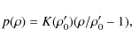
where
The density dependence of the bulk ![]() and shear
and shear ![]() moduli is modelled by a power law
moduli is modelled by a power law
Although according to Sirono (2004)
The time evolution of the pressure is directly given by the time
evolution of the density (Eq. (1)) and since
the pressure is a scalar quantity it is intrinsically invariant under
rotation. However, to gain a frame-invariant formulation of
the time evolution of the deviatoric stress tensor, i.e., the
stress rate, correction terms have to be added. A very common
formulation for SPH (see e.g., Benz & Asphaug 1994; Schäfer
et al. 2007) is the Jaumann rate form
where
and
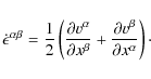
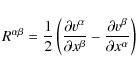
To determine rotation rate and strain rate tensor and thus the evolution of the stress tensor Eq. (10) in SPH representation, the SPH velocity derivatives
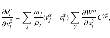
where the correction tensor
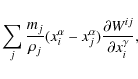
|
(14) |
that is
|
(15) |
This approach leads by construction to first order consistency where the errors caused by particle disorder cancel out and the conservation of angular momentum is ensured. Only this allows rigid rotation to be simulated correctly.
Finally, the sound speed of the material is given by
Together with Eq. (9), this relation shows that the sound speed is a strong function of density. This behaviour has been seen in molecular dynamics simulations by Paszun & Dominik (2008), but there is no data available from laboratory measurements.
Up to this point the set of equations describes a perfectly
elastic solid body. Additionally, the material simulated in this work
are ![]() dust aggregates, which have a high degree of porosity and, thus,
plasticity. The modifications that account for these features are
described in the next section.
dust aggregates, which have a high degree of porosity and, thus,
plasticity. The modifications that account for these features are
described in the next section.
2.3 Porosity and plasticity
Following the Sirono (2004)
model, the porosity ![]() is modelled by the density of the porous material
is modelled by the density of the porous material ![]() and the constant matrix density
and the constant matrix density
![]()
|
(17) |
In the following, we use the filling factor
We model plasticity by reducing inner stresses given
by
![]() .
For this reason, we need constitutive relations describing the
behaviour of the material during plastic deformation. These relations
are specific for each material and have to be determined empirically.
For highly porous materials it is particularly difficult to acquire
them. Therefore, it is advantageous that the model is based on
measurements by Blum &
Schräpler (2004), Blum
et al. (2006), and Güttler
et al. (2009).
.
For this reason, we need constitutive relations describing the
behaviour of the material during plastic deformation. These relations
are specific for each material and have to be determined empirically.
For highly porous materials it is particularly difficult to acquire
them. Therefore, it is advantageous that the model is based on
measurements by Blum &
Schräpler (2004), Blum
et al. (2006), and Güttler
et al. (2009).
The main idea of the adopted plasticity model is to reduce
inner stress once the material
exceeds a certain plasticity criterion. In the elastic case,
described by Eqs. (7)
and (8),
inner stresses grow linearly with deformation. Hence, the material
returns to its original shape at vanishingly external
forces. Reducing inner stresses, i.e., deviating from the
elastic deformation path, reduces the internal ability of the material
to restore its original shape. Therefore, by means of stress
reduction, deformation becomes permanent, i.e., plastic.
Following and expanding the approach by Sirono
(2004), we treat the plasticity of the pure hydrostatic
pressure p and the deviatoric stress
tensor
![]() separately.
separately.
For the deviatoric stress tensor, we follow the approach by Benz & Asphaug (1995) and
Schäfer et al. (2007)
by assuming that our material is isotropic, which makes the
von Mises yield criterion applicable. This criterion is
characterised by the shear strength Y,
which in our model is a composite of the compressive and tensile
strengths
![]() .
The suitability of this choice was already demonstrated in Güttler et al. (2009).
Since
.
The suitability of this choice was already demonstrated in Güttler et al. (2009).
Since ![]() is a scalar, we have to derive a scalar quantity from
is a scalar, we have to derive a scalar quantity from
![]() for reasons of comparability.
We do this by calculating its second irreducible invariant
for reasons of comparability.
We do this by calculating its second irreducible invariant
![]() .
Finally, the reduction of the deviatoric stress is implemented in the
following way
.
Finally, the reduction of the deviatoric stress is implemented in the
following way

|
(18) |
where
For
![\begin{figure}
\par\includegraphics[width=8.8cm,clip]{13596f01.eps}
\end{figure}](/articles/aa/full_html/2010/05/aa13596-09/img82.png)
|
Figure 1:
In the modified Sirono porosity model the regime of elastic deformation
is limited by the compressive strength
|
| Open with DEXTER | |
The pressure reduction process is implemented such that, at each time
step, p is computed using Eq. (8).
If, for a given, ![]()
![]() and
and
![]() ,
then the pressure
,
then the pressure ![]() is reduced to
is reduced to
![]() .
The deformation becomes irreversible once the new reference
density
.
The deformation becomes irreversible once the new reference
density ![]() is computed using Eq. (8) and
the elastic path is shifted towards higher densities. Hereby
the limiting filling factors
is computed using Eq. (8) and
the elastic path is shifted towards higher densities. Hereby
the limiting filling factors
![]() and
and
![]() are also set anew.
In principal, there are two possible
implementations of this: (1) plasticity becomes effective
immediately and
are also set anew.
In principal, there are two possible
implementations of this: (1) plasticity becomes effective
immediately and ![]() is computed whenever
is computed whenever ![]() ;
and (2) plasticity becomes effective after pressure decrease,
which is equivalent to
;
and (2) plasticity becomes effective after pressure decrease,
which is equivalent to
![]() .
We tested both implementations. For our understanding, possibility
(1) is closer to the underlying physical process.
In addition, it has proven to be more stable.
According to the benchmark parameters, the results were equivalent.
.
We tested both implementations. For our understanding, possibility
(1) is closer to the underlying physical process.
In addition, it has proven to be more stable.
According to the benchmark parameters, the results were equivalent.
For the tensile regime, i.e., for
![]() ,
we do not adopt the damage and damage-restoration model presented in Sirono (2004). This damage
model for brittle material such as rocks or pumice was developed for
SPH by Benz
& Asphaug (1994,1995) and used by Jutzi (2008) and Jutzi
et al. (2009,2008). It is assumed
that a material contains flaws, which are activated and develop under
tensile loading (Grady & Kipp
1980). Schäfer
et al. (2007) found that the model is not applicable
to their simulations of porous ice because it includes compressive
damage effects. Brittle material such as pumice and rocks tend to
disintegrate when compressed, i.e., they are crushed.
In contrast in our material of highly porous
,
we do not adopt the damage and damage-restoration model presented in Sirono (2004). This damage
model for brittle material such as rocks or pumice was developed for
SPH by Benz
& Asphaug (1994,1995) and used by Jutzi (2008) and Jutzi
et al. (2009,2008). It is assumed
that a material contains flaws, which are activated and develop under
tensile loading (Grady & Kipp
1980). Schäfer
et al. (2007) found that the model is not applicable
to their simulations of porous ice because it includes compressive
damage effects. Brittle material such as pumice and rocks tend to
disintegrate when compressed, i.e., they are crushed.
In contrast in our material of highly porous ![]() dust, both the tensile and compressive strengths increase with
compression. This is because the monomers are able to form new bonds
when they come into contact. Therefore, we adopt the same approach as
in the
compressive regime and reduce the pressure
dust, both the tensile and compressive strengths increase with
compression. This is because the monomers are able to form new bonds
when they come into contact. Therefore, we adopt the same approach as
in the
compressive regime and reduce the pressure ![]() to
to ![]() once the tensile strength is exceeded. Finally, the material can
rupture because of the plastic flow. However, material that is
plastically stretched can be compressed again up to its full strength.
By choosing this approach, a ``damage restoration
model'' is implemented in a very natural way.
once the tensile strength is exceeded. Finally, the material can
rupture because of the plastic flow. However, material that is
plastically stretched can be compressed again up to its full strength.
By choosing this approach, a ``damage restoration
model'' is implemented in a very natural way.
Finally, a remark has to be made about energy. Apart from
energy dissipation by numerical
and artificial viscosity, we assume intrinsic energy conservation. We
suppose that heat production in the investigated physical processes is
negligible. Therefore, our model is limited to a velocity regime below
the sound speed ![]() of the dust material (
of the dust material (![]() 30 m/s,
see Blum
& Wurm 2008; Paszun & Dominik 2008).
By choosing the approach to modelling plasticity that involves
stress reduction, we assume that most of the energy is dissipated by
plastic deformation, since the reduction in internal stresses accounts
for the reduction in internal energy.
30 m/s,
see Blum
& Wurm 2008; Paszun & Dominik 2008).
By choosing the approach to modelling plasticity that involves
stress reduction, we assume that most of the energy is dissipated by
plastic deformation, since the reduction in internal stresses accounts
for the reduction in internal energy.
Since we do not solve the energy equation thermodynamically enhanced features such as any phase transition such as melting and freezing cannot be simulated. This scheme also does not feature a damage model. When considering fragmentation (Sect. 5.3) in particular, any flaws in the material cannot yet be taken into account, although they might influence the resulting fragment distribution.
3 Experimental reference
3.1 Material parameters
The material used in the calibration experiments are highly-porous dust
aggregates as described by Blum
& Schräpler (2004), consisting of
spherical SiO2 spheres with a diameter
of 1.5 ![]() m.
For these clearly defined dust aggregates, it is possible to
reproducibly measure macroscopic material
parameters such as tensile strength, compressive strength, and,
potentially, also the shear strength needed for the
SPH porosity model (see Sect. 2.3).
The tensile strength of this material was measured for highly porous
and compacted aggregates (
m.
For these clearly defined dust aggregates, it is possible to
reproducibly measure macroscopic material
parameters such as tensile strength, compressive strength, and,
potentially, also the shear strength needed for the
SPH porosity model (see Sect. 2.3).
The tensile strength of this material was measured for highly porous
and compacted aggregates (
![]() )
by Blum & Schräpler (2004).
These measurements support a linear dependence between the tensile
strength and the number of contacts per monomer (increasing with
increasing
)
by Blum & Schräpler (2004).
These measurements support a linear dependence between the tensile
strength and the number of contacts per monomer (increasing with
increasing ![]() ),
which yields the tensile strength as
),
which yields the tensile strength as
The compressive strength was measured in the experimental counterpart of this paper (Güttler et al. 2009) with an experimental setup to determine the static omni-directional compression (ODC), whereby the sample is enclosed from all sides and the pressure is constant within the sample. We found that the compressive strength curve can be well described by the analytic function
where the free parameters were measured to be
3.2 Calibration experiment
As a setup for an easy and well-defined calibration experiment (see Güttler et al. 2009), we chose a glass bead with a diameter of 1 to 3 mm, which impacts into the dust aggregate material with a velocity of between 0.1 and 1 m s-1 under vacuum conditions (pressure 0.1 mbar). We were able to measure the deceleration curve, stopping time, and intrusion depth of the glass bead (for various velocities and projectile diameters) and the compaction of the dust under the glass bead (for a 1.1 mm projectile with a velocity of 0.65 m s-1). These results help us to calibrate and test the SPH code.
For the measurement of the deceleration curve, we used an
elongated epoxy projectile instead of the glass bead. The bottom shape
and the mass resembled the glass bead, while the lower density and the
therefore longer extension made it possible to observe the projectile
during the intrusion. The projectile was observed by a high-speed
camera (12 000 frames per second) and the position of
the upper edge was followed with an accuracy of
![]() m.
We found
that - independently of velocity and projectile
diameter - the intrusion curve can be described by a sine
curve
m.
We found
that - independently of velocity and projectile
diameter - the intrusion curve can be described by a sine
curve
where, D and
For the intrusion depth, we found good agreement with a linear
behaviour of
where v is the impact velocity of the projectile and m and
The compaction of dust underneath the impacted glass bead was
measured by X-ray micro-tomography. The glass bead diameter and
velocity in these experiments corresponded to the compaction
calibration setup described in Table 1.
The dust sample with an embedded glass bead was positioned onto a
rotatable sample carrier between an X-ray source and the detector.
During the rotation through
![]() ,
400 transmission images were taken, from which we computed
a 3D density reconstruction with a spatial resolution
of 21
,
400 transmission images were taken, from which we computed
a 3D density reconstruction with a spatial resolution
of 21 ![]() m.
The corresponding results for the density reconstruction can be found
in Güttler et al. (2009),
where we found that roughly one sphere volume beneath the glass bead is
compressed to a volume-filling factor of
m.
The corresponding results for the density reconstruction can be found
in Güttler et al. (2009),
where we found that roughly one sphere volume beneath the glass bead is
compressed to a volume-filling factor of
![]() ,
while the surrounding volume is nearly unaffected with an original
volume-filling factor of
,
while the surrounding volume is nearly unaffected with an original
volume-filling factor of
![]() .
In this work, we focus on the vertical density profile through
the centre of the sphere and the compressed material
(see Sect. 4).
.
In this work, we focus on the vertical density profile through
the centre of the sphere and the compressed material
(see Sect. 4).
Table 1: Numerical parameters for the compaction calibration setup.
3.3 Additionaly benchmark experiments
We present two additional experiments used to validate the
SPH code in Sects. 5.2
and 5.3.
Heißelmann et al.
(2007) performed low-velocity collisions (v=0.4 m s-1)
between cubic-shaped, approximately 5 mm-sized aggregates of
the
material as described in Sect. 3.1
and found bouncing whereby about 95% of the energy was
dissipated in a central collision. Detailed investigation of the
compaction in these collisions (Weidling
et al. 2009) revealed significant compaction of the
aggregates
(from ![]() to
to ![]() )
after approximately 1000 collisions. The energy needed for
this compaction is consistent with the energy dissipation measured by Heißelmann et al.
(2007).
)
after approximately 1000 collisions. The energy needed for
this compaction is consistent with the energy dissipation measured by Heißelmann et al.
(2007).
![\begin{figure}
\par\includegraphics[angle=90,width=8.5cm,clip]{13596f02.eps}
\end{figure}](/articles/aa/full_html/2010/05/aa13596-09/img126.png)
|
Figure 2: Cumulative mass distribution of the fragments after a disruptive collision, which can be described by a power law. The divergence at low masses is caused by the depletion of small aggregates because of the camera resolution. |
| Open with DEXTER | |
An additional experiment deals with the disruptive fragmentation of
dust aggregates
(for details, see Güttler et al. 2010,2009).
In this case, a dust aggregate with a diameter of
0.57 mm consisting of 1.5 ![]() m spherical SiO2
dust with a volume-filling factor of
m spherical SiO2
dust with a volume-filling factor of ![]() collides with a
solid glass target at a velocity of 8.4 m s-1
(also see Fig. 20
in Güttler et al. 2009).
The projectile fragments and the projected sizes of these fragments are
measured with a high-speed camera with a resolution of 16
collides with a
solid glass target at a velocity of 8.4 m s-1
(also see Fig. 20
in Güttler et al. 2009).
The projectile fragments and the projected sizes of these fragments are
measured with a high-speed camera with a resolution of 16 ![]() m per pixel.
As the mass measurement is restricted to the
2D images, the projected area of each fragment is
averaged over a sequence of images, where it is clearly separated from
other fragments. From this projected area, the fragment masses
are calculated with the assumptions of a spherical shape and an
unchanged volume filling factor. Figure 2 shows
the mass distribution in a cumulative plot. For higher masses,
which are not depleted by the finite camera resolution, we find good
agreement with a power-law distribution
m per pixel.
As the mass measurement is restricted to the
2D images, the projected area of each fragment is
averaged over a sequence of images, where it is clearly separated from
other fragments. From this projected area, the fragment masses
are calculated with the assumptions of a spherical shape and an
unchanged volume filling factor. Figure 2 shows
the mass distribution in a cumulative plot. For higher masses,
which are not depleted by the finite camera resolution, we find good
agreement with a power-law distribution
where m is the normalised mass (fragment mass divided by projectile mass) and
4 Numerical issues
Before we perform the calibration process, some numerical issues have to be resolved. For instance, it is unfeasible to simulate the dust sample, into which the glass bead drops in the compaction calibration experiment presented in Sect. 3, as a whole. It is also infeasible to carry out all necessary computations in 3D. Therefore, we simulate only part of the dust sample and attempt to determine the size at which spurious boundary effects emerge. Most of the calibration process was conducted in 2D, but the differences between 2D and 3D results are discussed and quantified.
In this context, we use the results of 2D simulations in cartesian coordinates, although the symmetry of the problem would be more accurately described by cylindrical coordinates. However, the SPH scheme in cylindrical or polar coordinates battles with the problem of a singularity at the origin of the kernel function. There have been only a few attempts to resolve this issue (e.g., Omang et al. 2006), which, however remain under development and require high implementation efforts. In our case, since 2D simulations provide only an indication of the calibration required and 3D simulations are aimed at, we stick to cartesian coordinates.
The glass bead is simulated with the Murnaghan equation
of state
![\begin{displaymath}%
p(\rho) = \left( \frac{K_0}{n} \right)
\left[ \left( \frac{\rho}{\rho_0} \right)^n - 1 \right],
\end{displaymath}](/articles/aa/full_html/2010/05/aa13596-09/img130.png)
|
(25) |
following the usual laws of continuum mechanics as presented in Sect. 2.2. The compaction calibration setup is initialised with the numerical parameters shown in Table 1, unless stated otherwise in the text. Our tests showed that the maximum intrusion depth and the density profile are the calibration parameters most sensitive to changes in the numerical setup. Density profiles (e.g., Figs. 4 and 5) display the filling factor
![\begin{figure}
\par\includegraphics[width=6cm,clip]{13596f03.eps}
\end{figure}](/articles/aa/full_html/2010/05/aa13596-09/img131.png)
|
Figure 3:
Compaction calibration setup in 2D or, respectively,
cross-section of 3D compaction calibration setup.
A glass sphere impacts into a dust sample (radius
|
| Open with DEXTER | |
4.1 Computational domain and boundary conditions
In 2D simulations, we tested the effect of changing the size and shape
of the dust sample. Initially the particles were set on a triangular
lattice with a lattice constant of 25 ![]() .
To be geometrically consistent with the cylindric experimental
setup, we firstly utilised a box (width 8 mm) and
varied its depth: 1.375 mm, 2.2 mm, 3.3 mm,
and 5.5 mm. This is equivalent to the dimensions
.
To be geometrically consistent with the cylindric experimental
setup, we firstly utilised a box (width 8 mm) and
varied its depth: 1.375 mm, 2.2 mm, 3.3 mm,
and 5.5 mm. This is equivalent to the dimensions
![]() ,
,
![]() ,
,
![]() ,
and 10
,
and 10 ![]()
![]() .
Comparing the density profiles (Fig. 4,
top), two features are remarkable: (1) the maximum filling
factor at the top of the dust sample (
.
Comparing the density profiles (Fig. 4,
top), two features are remarkable: (1) the maximum filling
factor at the top of the dust sample (
![]() at
at
![]() )
and the intrusion depth D is nearly the
same for all dust sample sizes. (2) For
)
and the intrusion depth D is nearly the
same for all dust sample sizes. (2) For
![]() ,
we find spurious density peaks at the lower boundaries (
,
we find spurious density peaks at the lower boundaries (
![]() and
and
![]() ).
).
To reduce the computation time, we simulated the dust sample
as a semicircle with the same radius variation as above. The resulting
density profiles are shown in Fig. 4
(bottom). In contrast to the corresponding simulations with
the box-shaped samples, we find for
![]() an increased maximum filling factor and a slightly reduced intrusion
depth. Because of the greater amount of volume lateral to the
intrusion channel, material can be pushed aside more easily than inside
the narrow boundaries of the semicircle. Therefore, a higher
fraction of the material is compressed to higher filling factors.
For
an increased maximum filling factor and a slightly reduced intrusion
depth. Because of the greater amount of volume lateral to the
intrusion channel, material can be pushed aside more easily than inside
the narrow boundaries of the semicircle. Therefore, a higher
fraction of the material is compressed to higher filling factors.
For
![]() ,
the spurious boundary effects become negligible within the compaction
calibration setup and the density structure shows no significant
difference for box-shaped and semicircle-shaped dust samples.
,
the spurious boundary effects become negligible within the compaction
calibration setup and the density structure shows no significant
difference for box-shaped and semicircle-shaped dust samples.
Hence, all computations of Sect. 4 are
conducted on the basis of a semicircle in 2D or a hemisphere
in 3D with a radius of
![]() .
.
In all cases, the dust sample is bordered by a few layers of
boundary particles. The acceleration of these particles is set to zero
at each integration step, simulating reflecting boundary conditions.
Apart from that, i.e., in terms of the equation of
state, they are treated like dust particles. We also tested damping
boundary conditions by simulating two layers of boundaries. The outer
layer was treated as described above, the inner (sufficiently large)
layer was simulated with a high artificial ![]() -viscosity. Since there was no
significant difference in the outcome, we fix all boundaries
in the aforementioned way and consider them to be reflecting.
-viscosity. Since there was no
significant difference in the outcome, we fix all boundaries
in the aforementioned way and consider them to be reflecting.
![\begin{figure}
\par\includegraphics[angle=-90,width=8cm,clip]{13596f04.ps}\vspace*{3mm}
\includegraphics[angle=-90,width=8cm,clip]{13596f05.ps}
\end{figure}](/articles/aa/full_html/2010/05/aa13596-09/img146.png)
|
Figure 4:
Vertical density profile at maximum intrusion for the compaction
calibration setup and different shapes of the 2D dust sample
(box and semicircle).
Depth
|
| Open with DEXTER | |
4.2 Resolution and Convergence
Jutzi (2008) found in his studies of a basalt sphere impacting a porous target that the outcome of his simulations strongly depended on their resolutions. With a calibration setup similar to that used in this paper, Geretshauser (2006) confirms that in simulations of the type presented in this work, a strong resolution dependence is present. He found that the intrusion depth of the glass bead can be doubled by doubling the resolution. Since the calibration experiments presented in Güttler et al. (2009) are extremely sensitive even to minor changes in the setup, the convergence properties of porosity model and the underlying SPH method are investigated carefully in this paragraph. Additionally, we study the differences in the outcome of 2D and 3D setup.
For the 2D convergence study, particles were initially placed
on a triangular lattice again. The lattice constants ![]() were 100, 50, 25, and 12.5
were 100, 50, 25, and 12.5 ![]() for the compaction calibration setup. The smoothing length h
was kept constant relative to
for the compaction calibration setup. The smoothing length h
was kept constant relative to ![]() at a ratio of 5.6
at a ratio of 5.6 ![]()
![]() .
The maximum number of interaction partners was
.
The maximum number of interaction partners was
![]() ,
the average
,
the average
![]() ,
and the minimum
,
and the minimum ![]() .
.
![\begin{figure}
\par\includegraphics[angle=-90,width=8cm,clip]{13596f06.ps}\vspace*{3mm}
\includegraphics[angle=-90,width=8cm,clip]{13596f07.ps}
\end{figure}](/articles/aa/full_html/2010/05/aa13596-09/img151.png)
|
Figure 5: Convergence study of the vertical density profile for 2D ( top) and 3D ( bottom) compaction calibration setups. The increase in filling factor towards the surface of the dust sample accounts for the glass bead, which is not removed in this plot. Simulations were performed for different spatial resolutions. All curves show a characteristic filling-factor minimum between the sphere and dust sample and a characteristic filling-factor maximum indicating the dust sample surface. |
| Open with DEXTER | |
In the 3D convergence study, we used a cubic lattice with edge lengths ![]() =
100, 50, and 25
=
100, 50, and 25 ![]() .
The latter was simulated with 3.7 million
SPH particles, which represent the limit of our computational
resources. We fixed h = 3.75
.
The latter was simulated with 3.7 million
SPH particles, which represent the limit of our computational
resources. We fixed h = 3.75 ![]()
![]() ,
which yielded
,
which yielded ![]() ,
,
![]() ,
and
,
and ![]() .
The results are presented in Fig. 5.
In contrast to the plots in Fig. 4,
the glass sphere is not removed here. Coming from the right side of the
plot, the filling factor rapidly decreases from a high value beyond the
edge of the plot describing the sphere. The filling factor reaches its
minimum at an artificial gap between sphere and surface of the dust
sample.
The width of this gap is about one smoothing length h.
The existence of the gap has two reasons: (1) sphere material
and dust material have to be separated by artificial viscosity for
stability reasons. This is discussed below. (2) The volume of
the sphere represents an area of extremely high density and pressure
with respect to the dust sample. This area is smoothed out by the
SPH method, the width of the smoothing being given by the
smoothing length. Although clear convergence behaviour is evident in
Fig. 5
for both the 2D and the 3D case, a more unique
convergence criterion has to be found. For this purpose, we
choose the maximum intrusion depth, which proved to be very sensitive
to resolution changes. The shape of the filling-factor profile provides
two ways to determine the intrusion depth: (1) the filling
factor minimum, which is inbetween sphere and dust sample; and
(2) the filling factor maximum (peak) of the dust material
left in the gap between sphere and dust sample.
.
The results are presented in Fig. 5.
In contrast to the plots in Fig. 4,
the glass sphere is not removed here. Coming from the right side of the
plot, the filling factor rapidly decreases from a high value beyond the
edge of the plot describing the sphere. The filling factor reaches its
minimum at an artificial gap between sphere and surface of the dust
sample.
The width of this gap is about one smoothing length h.
The existence of the gap has two reasons: (1) sphere material
and dust material have to be separated by artificial viscosity for
stability reasons. This is discussed below. (2) The volume of
the sphere represents an area of extremely high density and pressure
with respect to the dust sample. This area is smoothed out by the
SPH method, the width of the smoothing being given by the
smoothing length. Although clear convergence behaviour is evident in
Fig. 5
for both the 2D and the 3D case, a more unique
convergence criterion has to be found. For this purpose, we
choose the maximum intrusion depth, which proved to be very sensitive
to resolution changes. The shape of the filling-factor profile provides
two ways to determine the intrusion depth: (1) the filling
factor minimum, which is inbetween sphere and dust sample; and
(2) the filling factor maximum (peak) of the dust material
left in the gap between sphere and dust sample.
![\begin{figure}
\par\includegraphics[angle=-90,width=8cm,clip]{13596f08.ps}\vspace*{2mm}
\includegraphics[angle=-90,width=8cm,clip]{13596f09.ps}
\end{figure}](/articles/aa/full_html/2010/05/aa13596-09/img157.png)
|
Figure 6:
Convergence study of the maximum intrusion depth for the 2D (
top) and 3D ( bottom) compaction
calibration setups. Filled symbols represent the position of the
filling factor peak of the dust material, whereas empty symbols denote
the position of the minimum filling factor at the gap between glass
bead and dust material. The values are derived from the density
profiles in Fig. 5.
The smoothing length is indicated by the error bars. While the peak
position remains almost constant at
|
| Open with DEXTER | |
Figure 6
shows the results for both cases in 2D (top) and
3D (bottom). The error bars around the minimum values
represent the smoothing length and provide an indication of the maximum
error. The position of the density peak remains almost constant,
converging to ![]() (2D)
and
(2D)
and ![]() (3D),
respectively, at higher resolutions. The position of the
density minimum at low resolutions differs significantly from the
position of the density peak, but converges quickly to the
same intrusion depth at higher resolutions. However, the differences
between the extrema remain well within one smoothing length. This is
because the sphere and dust sample are separated by about one smoothing
length. Comparing 2D and 3D convergence,
the 3D case seems to converge more quickly.
(3D),
respectively, at higher resolutions. The position of the
density minimum at low resolutions differs significantly from the
position of the density peak, but converges quickly to the
same intrusion depth at higher resolutions. However, the differences
between the extrema remain well within one smoothing length. This is
because the sphere and dust sample are separated by about one smoothing
length. Comparing 2D and 3D convergence,
the 3D case seems to converge more quickly.
Because of the findings of this study, we choose a spatial
resolution of ![]() for additional simulations in 2D. In the
3D case,
for additional simulations in 2D. In the
3D case, ![]() is sufficient,
but
is sufficient,
but ![]() is desirable if feasible. After defining suitable values for the
spatial resolution, we now turn to the numerical resolution, which for
the SPH scheme is given by the number of interaction partners
of each single particle. For the investigation of this feature, we
performed a study utilising the 2D compaction calibration
setup with a spatial resolution of
is desirable if feasible. After defining suitable values for the
spatial resolution, we now turn to the numerical resolution, which for
the SPH scheme is given by the number of interaction partners
of each single particle. For the investigation of this feature, we
performed a study utilising the 2D compaction calibration
setup with a spatial resolution of
![]() and varied the ratio of smoothing length to lattice constant
and varied the ratio of smoothing length to lattice constant
![]() from 2 to 7
in steps of one, where
from 2 to 7
in steps of one, where
![]() determines the initial number
of interaction partners that is smoothed
over. The resulting maximum, average, and minimum
interactions
determines the initial number
of interaction partners that is smoothed
over. The resulting maximum, average, and minimum
interactions
![]() ,
,
![]() ,
and
,
and
![]() and the corresponding
smoothing lengths h
can be found in Table 2.
Additionally, we measured the time
and the corresponding
smoothing lengths h
can be found in Table 2.
Additionally, we measured the time
![]() the computations took,
simulated on 4 cores of a cluster with
Intel Xenon Quad-Core processors (2.66 GHz) for a simulated
time of
the computations took,
simulated on 4 cores of a cluster with
Intel Xenon Quad-Core processors (2.66 GHz) for a simulated
time of ![]() and the number of integration steps
and the number of integration steps
![]() of our adaptive Runge-Kutta
Cash-Karp integrator.
of our adaptive Runge-Kutta
Cash-Karp integrator.
Table 2: Parameters for the convergence study regarding interaction numbers.
![\begin{figure}
\par\includegraphics[angle=-90,width=8cm,clip]{13596f10.ps}
\end{figure}](/articles/aa/full_html/2010/05/aa13596-09/img171.png)
|
Figure 7:
Convergence study for the density profile using the 2D setup
and varying the smoothing length h. Through
this variation, the number of interaction partners is varied according
to Table 2.
The glass bead has been removed in this plot. For
|
| Open with DEXTER | |
Comparing the density profiles in Fig. 7
(where the glass bead has been removed), instabilities in the form of
filling factor fluctuations due to insufficient interaction numbers
appear for smoothing lengths
![]() ,
i.e., for
,
i.e., for ![]() .
For
.
For ![]() ,
the density profile has essentially the same shape:
the position and height of the filling factor peak remains
nearly the same and
,
the density profile has essentially the same shape:
the position and height of the filling factor peak remains
nearly the same and ![]() drops
smoothly to
drops
smoothly to
![]() towards the bottom of the dust
sample. Only the sharp edge at the top
of the dust sample is smoothed across a wider range due to the
increased smoothing length.
towards the bottom of the dust
sample. Only the sharp edge at the top
of the dust sample is smoothed across a wider range due to the
increased smoothing length.
Table 2
shows that the number of integration steps
![]() decreases with increasing
interaction numbers. This is because
the elastic waves inside the dust sample are smoothed over a wider
range causing the adaptive integrator to increase the duration of a
time step, since density fluctuations do not have to be resolved as
sharply as when a lower amount of smoothing is applied.
As expected, the computation time
decreases with increasing
interaction numbers. This is because
the elastic waves inside the dust sample are smoothed over a wider
range causing the adaptive integrator to increase the duration of a
time step, since density fluctuations do not have to be resolved as
sharply as when a lower amount of smoothing is applied.
As expected, the computation time
![]() generally increases with the
increasing number of interactions. There
are two exceptions:
generally increases with the
increasing number of interactions. There
are two exceptions: ![]() and
and ![]() .
Here, the decrease in
.
Here, the decrease in
![]() overcompensates for the
increase in the interactions leading to a
decrease in
overcompensates for the
increase in the interactions leading to a
decrease in
![]() .
Hence, a ratio
.
Hence, a ratio
![]() yields
the necessary accuracy and an acceptable amount of computation time.
This study also justifies the choice of
yields
the necessary accuracy and an acceptable amount of computation time.
This study also justifies the choice of
![]() in Güttler et al. (2009)
and we use this ratio throughout this paper.
in Güttler et al. (2009)
and we use this ratio throughout this paper.
According to these findings, for 3D simulations an
average interaction number of theoretically
![]() would be needed to achieve the same numerical resolution. However,
similar simulations are infeasible and our choice of
would be needed to achieve the same numerical resolution. However,
similar simulations are infeasible and our choice of
![]() in 3D is equivalent to
in 3D is equivalent to
![]() in 2D, which should provide sufficient and reliable accuracy.
in 2D, which should provide sufficient and reliable accuracy.
4.3 Geometrical difference - 2D and 3D setups
As one can easily see in Fig. 6,
2D and 3D simulations have significantly different
convergence values for the intrusion depth. This deviation is caused by
the geometrical difference of the 2D and 3D setup.
The 2D setup (glass circle impacts into dust
semicircle) represents a slice through a glass cylinder and a
semi-cylindrical dust sample, which
implies an infinite expansion into the third spatial direction.
In contrast the 3D setup represents a real sphere
dropping into a ``bowl'' of dust. The relation for the
intrusion depth found by Güttler
et al. (2009) (see Sect. 3)
contains a geometrical dependence
![]() ,
where D is the intrusion depth, m is
the mass of the impacting glass bead, v is
its impact velocity, A is its
cross-section, and
,
where D is the intrusion depth, m is
the mass of the impacting glass bead, v is
its impact velocity, A is its
cross-section, and
![]() is the mass per unit length. Güttler
et al. (2009) applied this relation to determine a
rough correction factor between 2D and 3D simulation
setups:
is the mass per unit length. Güttler
et al. (2009) applied this relation to determine a
rough correction factor between 2D and 3D simulation
setups:
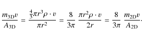
Hence, the 2D intrusion depth has to be corrected by a factor of
![\begin{figure}
\par\includegraphics[angle=-90,width=7.8cm,clip]{13596f11.ps}
\end{figure}](/articles/aa/full_html/2010/05/aa13596-09/img188.png)
|
Figure 8: Verification of the 2D-3D correction factor. Filled symbols denote the position of the filling factor peak of the dust material in Fig. 5. Triangles represent 3D and squares 2D values. The conversion from 2D to 3D intrusion depth utilising the correction factor from Eqs. (26) and (23) due to the geometrical difference is indicated by the line without symbols. The 3D values are in very good agreement with the very rough theoretical prediction. They lie well within the errors. |
| Open with DEXTER | |
4.4 Artificial viscosity
Since artificial viscosity plays an eminent role in the stability of
SPH simulations, we investigate its influence on the outcome
of our compaction calibration setup. Only artificial ![]() -viscosity
is applied in our test case, but in a threefold way: (1) it
dampens high oscillation modes of the glass bead caused by the stiff
Murnaghan equation of state (EOS). Thereby it enlarges the time step of
our adaptive integrator and saves computation time.
(2) It is used to provide the dust material with a
basic stability. (3) It separates the areas of Murnaghan EOS
and dust EOS and prevents a so-called ``cannonball instability''. For
all three cases, the influence of
-viscosity
is applied in our test case, but in a threefold way: (1) it
dampens high oscillation modes of the glass bead caused by the stiff
Murnaghan equation of state (EOS). Thereby it enlarges the time step of
our adaptive integrator and saves computation time.
(2) It is used to provide the dust material with a
basic stability. (3) It separates the areas of Murnaghan EOS
and dust EOS and prevents a so-called ``cannonball instability''. For
all three cases, the influence of ![]() -artificial viscosity was also
tested, but its influence on all benchmark parameters was found to be
negligible.
-artificial viscosity was also
tested, but its influence on all benchmark parameters was found to be
negligible.
(1) The choice of the ![]() -viscosity of the glass
bead proved to be unimportant. We choose the canonical value
-viscosity of the glass
bead proved to be unimportant. We choose the canonical value
![]() .
No influence on the physical benchmark parameters was detected
for all
.
No influence on the physical benchmark parameters was detected
for all ![]() values,
except
values,
except ![]() ,
which produces an instability. Values of
,
which produces an instability. Values of
![]() have no significant effect on the damping, and the influence for
have no significant effect on the damping, and the influence for
![]() is not too high, but still observable. Hence, we stick to the canonical
value.
is not too high, but still observable. Hence, we stick to the canonical
value.
(2) Sirono (2004)
applies no artificial viscosity to his porous ice material because of
its spurious dissipative properties. Our findings, shown in
Fig. 9,
qualify this choice in terms of the dust material.
Within our 2D compaction calibration setup (
![]() ,
,
![]() ),
we vary
),
we vary ![]() from 0 to 2 and observe its influence on the density
profile (Fig. 9,
top) and the maximum intrusion represented by the filling factor peak
of the dust material (Fig. 9, bottom).
from 0 to 2 and observe its influence on the density
profile (Fig. 9,
top) and the maximum intrusion represented by the filling factor peak
of the dust material (Fig. 9, bottom).
The position of the filling factor peak ranges from ![]()
![]() with
with
![]() to
to ![]() at
at ![]() .
This clearly demonstrates the dissipative feature of the
.
This clearly demonstrates the dissipative feature of the ![]() -viscosity,
since a lower amount of kinetic energy of the glass bead is transformed
into plastic deformation with higher
-viscosity,
since a lower amount of kinetic energy of the glass bead is transformed
into plastic deformation with higher ![]() .
The residual energy must have been dissipated. However, the
.
The residual energy must have been dissipated. However, the ![]() -viscosity-intrusion
curve seems to saturate at a value of
-viscosity-intrusion
curve seems to saturate at a value of
![]() .
The decrease in the maximum intrusion can also be seen in the
density profile (Fig. 9, top).
While the profile maintains nearly the same shape, the height of the
filling factor peak decreases with increasing
.
The decrease in the maximum intrusion can also be seen in the
density profile (Fig. 9, top).
While the profile maintains nearly the same shape, the height of the
filling factor peak decreases with increasing ![]() .
Hence, an increasing artificial viscosity diminishes the peak
pressure during compaction by means of the compressive strength
relation
.
Hence, an increasing artificial viscosity diminishes the peak
pressure during compaction by means of the compressive strength
relation
![]() ,
which is directly responsible for the height of the filling
factor peak.
,
which is directly responsible for the height of the filling
factor peak.
In contrast to Sirono
(2004), we find that it is necessary to apply a small amount
of ![]() -viscosity
to the dust material. For
-viscosity
to the dust material. For
![]() ,
the results show evidences of an instability, which is also responsible
for a rapid increase in the maximum intrusion. Therefore, we find it
convenient to apply an artificial viscosity with
,
the results show evidences of an instability, which is also responsible
for a rapid increase in the maximum intrusion. Therefore, we find it
convenient to apply an artificial viscosity with
![]() to the dust material, which holds for the previous simulations of this
section as well as the following. The choice of a non-zero
to the dust material, which holds for the previous simulations of this
section as well as the following. The choice of a non-zero ![]() ,
however, is also justified by experimental findings: after
impacting into the dust sample, the glass bead shortly
oscillates because of the elastic properties of the dust. This
oscillation is damped by internal friction, which we model with
artificial viscosity. Therefore, by choosing a
non-zero
,
however, is also justified by experimental findings: after
impacting into the dust sample, the glass bead shortly
oscillates because of the elastic properties of the dust. This
oscillation is damped by internal friction, which we model with
artificial viscosity. Therefore, by choosing a
non-zero ![]() we take into account the dissipative properties that our dust material
naturally has. A quantitative calibration of this parameter,
however, is left to future work.
we take into account the dissipative properties that our dust material
naturally has. A quantitative calibration of this parameter,
however, is left to future work.
(3) During our first simulations with the
2D compaction calibration setup, we observed what is sometimes
described in the literature as ``cannonball instability''. During the
compaction process, when the glass bead intrudes into the dust
material, single particles at the sphere's surface begin to oscillate
between the domains of the Murnaghan EOS and dust EOS. Because of the
significant difference in the ``stiffness'' of these two equations of
state, the particles acquire an enormous amount of kinetic
energy until they move fast enough to generate a pressure on the dust
material that exceeds the compressive strength
![]() .
Eventually they disengage from the sphere's surface like a cannonball
and dig themselves into the dust sample causing a huge amount of
unphysical compaction. We tackle this problem for all
SPH particles with dust EOS, which interact with glass bead
SPH particles, by applying the same amount of
.
Eventually they disengage from the sphere's surface like a cannonball
and dig themselves into the dust sample causing a huge amount of
unphysical compaction. We tackle this problem for all
SPH particles with dust EOS, which interact with glass bead
SPH particles, by applying the same amount of ![]() -viscosity
as for the sphere, i.e.,
-viscosity
as for the sphere, i.e.,
![]() .
In our simulations, this is sufficient to prevent the
``cannonball instability''. The spurious dissipation caused by this
measure is negligible.
.
In our simulations, this is sufficient to prevent the
``cannonball instability''. The spurious dissipation caused by this
measure is negligible.
![\begin{figure}
\par\includegraphics[angle=-90,width=7.7cm,clip]{13596f12.ps}\vspace*{1.5mm}
\includegraphics[angle=-90,width=7.7cm,clip]{13596f13.ps}
\end{figure}](/articles/aa/full_html/2010/05/aa13596-09/img201.png)
|
Figure 9:
Density profile ( top) and maximum intrusion (
bottom) for different values of artificial |
| Open with DEXTER | |
5 Calibration
5.1 Compressive strength and compaction properties
We refine and extend a study of the compaction properties of the dust
sample, which was already carried out in a similar, but less detailed
way in Güttler et al.
(2009). There the quantity having the strongest influence on
the compaction was found to be the compressive strength
relation
![]() (Eq. (21)),
which was measured in an omni-directional and static manner.
To adapt this relation to dynamic compression, the mean
pressure
(Eq. (21)),
which was measured in an omni-directional and static manner.
To adapt this relation to dynamic compression, the mean
pressure ![]() and the ``slope'' of the Fermi-shaped curve
and the ``slope'' of the Fermi-shaped curve ![]() can be treated as free parameters. The upper and lower boundaries of
the filling factor
can be treated as free parameters. The upper and lower boundaries of
the filling factor ![]() and
and ![]() ,
respectively, remain constant even in the dynamic case. Güttler et al. (2009)
found that by lowering
,
respectively, remain constant even in the dynamic case. Güttler et al. (2009)
found that by lowering ![]() ,
most of the features of the compaction calibration setup can
be reproduced in a very satisfactory manner.
As a result, the ratio of the filling factor to
compressive strength curve (see also Fig. 2 in Güttler et al. 2009)
is shifted towards lower pressures and the yield pressure for
compression is lowered. Using only 2D simulations and a rough
parameter grid, Güttler
et al. (2009) fix
,
most of the features of the compaction calibration setup can
be reproduced in a very satisfactory manner.
As a result, the ratio of the filling factor to
compressive strength curve (see also Fig. 2 in Güttler et al. 2009)
is shifted towards lower pressures and the yield pressure for
compression is lowered. Using only 2D simulations and a rough
parameter grid, Güttler
et al. (2009) fix
![]() .
The ``slope''
.
The ``slope'' ![]() has not been considered.
In this work, we consider
has not been considered.
In this work, we consider ![]() and we perform more accurate parameter studies for
and we perform more accurate parameter studies for ![]() .
From the latter, we predict a reasonable choice for
.
From the latter, we predict a reasonable choice for ![]() ,
which represents the basis of a 3D simulation of the
compaction calibration setup. The results of this simulation are later
compared to results from the laboratory. In this comparison,
we use the same features as Güttler
et al. (2009).
,
which represents the basis of a 3D simulation of the
compaction calibration setup. The results of this simulation are later
compared to results from the laboratory. In this comparison,
we use the same features as Güttler
et al. (2009).
5.1.1 Fixing free parameters
Since no empirical data are available for ![]() in the dynamical compressive strength curve, we perform a parameter
study to determine a suitable choice for this important quantity. For
this study, we use the 2D compaction calibration setup and
vary
in the dynamical compressive strength curve, we perform a parameter
study to determine a suitable choice for this important quantity. For
this study, we use the 2D compaction calibration setup and
vary ![]() from 0.13 to
from 0.13 to ![]() (Figs. 10
and 11),
where
(Figs. 10
and 11),
where ![]() represents the value of the static compressive strength curve. The
effect of lowering
represents the value of the static compressive strength curve. The
effect of lowering ![]() can most clearly be seen in the vertical filling-factor profile
(Fig. 10,
top). First of all, more material can be compressed and is to higher
filling factors. As a consequence, the glass
bead intrudes more deeply into the dust sample. From experimental
results, we expect an intrusion depth of about one sphere
diameter (
can most clearly be seen in the vertical filling-factor profile
(Fig. 10,
top). First of all, more material can be compressed and is to higher
filling factors. As a consequence, the glass
bead intrudes more deeply into the dust sample. From experimental
results, we expect an intrusion depth of about one sphere
diameter (
![]() ). With the aid of the
empirical relation between the ratio of momentum to impactor
cross-section mvA-1
and
intrusion depth D (Eq. (23))
as well as the correction factor between 2D and
3D intrusion depth (Eq. (26)),
we estimate that
). With the aid of the
empirical relation between the ratio of momentum to impactor
cross-section mvA-1
and
intrusion depth D (Eq. (23))
as well as the correction factor between 2D and
3D intrusion depth (Eq. (26)),
we estimate that
![]() corresponds to
corresponds to
![]() .
Figure 11
shows the maximum intrusion over the stopping time for various values
of
.
Figure 11
shows the maximum intrusion over the stopping time for various values
of ![]() (labels). The estimated
(labels). The estimated ![]() is indicated by a dashed line. In terms of intrusion depth, we deduce
that a dynamic mean pressure
is indicated by a dashed line. In terms of intrusion depth, we deduce
that a dynamic mean pressure
![]() kPa
is a suitable choice.
kPa
is a suitable choice.
This is supported by the peak filling factor appearing in the
filling factor profile (Fig. 10,
bottom). For the compaction calibration setup, empirical data indicate
that a peak filling factor
![]() can be expected. The comparison between 2D and
3D results (Sect. 4.3)
has shown that the peak filling factor in the vertical density profile
in the 2D case is generally higher than for the same situation
in 3D. The equivalent of
can be expected. The comparison between 2D and
3D results (Sect. 4.3)
has shown that the peak filling factor in the vertical density profile
in the 2D case is generally higher than for the same situation
in 3D. The equivalent of
![]() is a maximum filling factor of
is a maximum filling factor of
![]() in 2D. This points to a choice of
in 2D. This points to a choice of
![]() ,
which is consistent with the findings for the intrusion depth.
,
which is consistent with the findings for the intrusion depth.
![\begin{figure}
\par\includegraphics[angle=-90,width=8cm,clip]{13596f14.ps}\vspace*{2mm}
\includegraphics[angle=-90,width=8cm,clip]{13596f15.ps}
\end{figure}](/articles/aa/full_html/2010/05/aa13596-09/img212.png)
|
Figure 10:
Density profile ( top) and maximum peak filling
factor from the density profile over |
| Open with DEXTER | |
![\begin{figure}
\par\includegraphics[angle=-90,width=7.7cm,clip]{13596f16.ps}
\end{figure}](/articles/aa/full_html/2010/05/aa13596-09/img213.png)
|
Figure 11:
Maximum intrusion over stopping time for different values of the mean
pressure |
| Open with DEXTER | |
![\begin{figure}
\includegraphics[angle=-90,width=7.7cm,clip]{13596f17.ps}\vspace*{1.5mm}
\includegraphics[angle=-90,width=8.5cm,clip]{13596f18.ps}
\end{figure}](/articles/aa/full_html/2010/05/aa13596-09/img214.png)
|
Figure 12:
Density profile ( top) and normalised volume
fraction of compacted volume over its corresponding filling factor (
bottom) for different values of |
| Open with DEXTER | |
The compressive strength relation
![]() (Eq. (21))
contains a second free parameter
(Eq. (21))
contains a second free parameter ![]() ,
which accounts for the ``slope'' of the Fermi-shaped curve.
In Güttler et al. (2009),
this parameter was chosen to be indentical to that of the static
omni-directional compressive strength curve and a more careful
investigation was not carried out. To understand its effect on
the compaction properties of the dust sample, we utilise the
2D compaction calibration setup again and vary
,
which accounts for the ``slope'' of the Fermi-shaped curve.
In Güttler et al. (2009),
this parameter was chosen to be indentical to that of the static
omni-directional compressive strength curve and a more careful
investigation was not carried out. To understand its effect on
the compaction properties of the dust sample, we utilise the
2D compaction calibration setup again and vary ![]() from 0.55 to 0.80. The results are presented in
Fig. 12.
From the vertical density profile (Fig. 12, top),
it can be seen that increasing
from 0.55 to 0.80. The results are presented in
Fig. 12.
From the vertical density profile (Fig. 12, top),
it can be seen that increasing ![]() increases the intrusion depth, but not as effectively as
lowering the mean pressure
increases the intrusion depth, but not as effectively as
lowering the mean pressure ![]() .
This is because increasing
.
This is because increasing ![]() hardly increases the peak filling factor in the vertical density
profile.
More volume is compressed to lower filling factors.
In contrast, by lowering
hardly increases the peak filling factor in the vertical density
profile.
More volume is compressed to lower filling factors.
In contrast, by lowering ![]() the total amount of volume compressed becomes smaller but is compacted
to higher filling factors. This behaviour can be seen by comparing the
density profiles for the
the total amount of volume compressed becomes smaller but is compacted
to higher filling factors. This behaviour can be seen by comparing the
density profiles for the ![]() variation
(Fig. 10,
top) and
variation
(Fig. 10,
top) and ![]() variation
(Fig. 12,
top) and
in particular from the cumulated volume over filling factor curve
(Fig. 12,
bottom). This figure shows the normalised fraction of compacted volume
corresponding to a volume filling factor
variation
(Fig. 12,
top) and
in particular from the cumulated volume over filling factor curve
(Fig. 12,
bottom). This figure shows the normalised fraction of compacted volume
corresponding to a volume filling factor ![]() .
The intersection of the curves with the y-axis
represents the total compressed volume, which is increased from
.
The intersection of the curves with the y-axis
represents the total compressed volume, which is increased from
![]() to
to
![]() sphere volumes. The
corresponding experimental measurements here infer a value of roughly
one sphere volume (see Sect. 3.2).
For
sphere volumes. The
corresponding experimental measurements here infer a value of roughly
one sphere volume (see Sect. 3.2).
For ![]() in particular the compacted volume fraction is increased. The
equivalent figure for the
in particular the compacted volume fraction is increased. The
equivalent figure for the ![]() variation can be
found in Güttler et al.
(2009, Fig. 15).
By comparing the 2D and 3D calibration setups
(Sect. 4.3),
we infer that a significant amount of this compaction (especially in
the lower filling factor regime) is caused by the geometrical
difference. However, the experimental data do not indicate a
particularly high amount of compaction to lower filling factors (rather
the contrary) and, therefore, we maintain our initial choice of
variation can be
found in Güttler et al.
(2009, Fig. 15).
By comparing the 2D and 3D calibration setups
(Sect. 4.3),
we infer that a significant amount of this compaction (especially in
the lower filling factor regime) is caused by the geometrical
difference. However, the experimental data do not indicate a
particularly high amount of compaction to lower filling factors (rather
the contrary) and, therefore, we maintain our initial choice of
![]() .
.
5.1.2 Comparison with experiments
To compare with experiments, we performed a simulation using the
3D compaction calibration setup (see Table 1)
with two exceptions: (1) the bulk modulus of the dust material
was set to ![]() (instead of
(instead of ![]() )
since findings presented below indicated a much lower bulk modulus.
However, the choice of K0
has little influence on the
compaction properties calibrated for in the compaction calibration
setup. It is more important for bouncing and fragmentation,
as shown below. (2) The mean pressure of the
compressive strength relation (Eq. (21))
was set to
)
since findings presented below indicated a much lower bulk modulus.
However, the choice of K0
has little influence on the
compaction properties calibrated for in the compaction calibration
setup. It is more important for bouncing and fragmentation,
as shown below. (2) The mean pressure of the
compressive strength relation (Eq. (21))
was set to ![]() as suggested in the previous section.
as suggested in the previous section.
The following features of the compaction calibration setup
were measured in the laboratory and are used here for comparison:
(1) the stopping time ![]() ;
(2) the intrusion curve of the projectile; (3) the
vertical density profile; (4) the cumulated volume over
filling factor curve; and (5) the cross-section through both
the sphere and the dust sample displaying the filling factor.
;
(2) the intrusion curve of the projectile; (3) the
vertical density profile; (4) the cumulated volume over
filling factor curve; and (5) the cross-section through both
the sphere and the dust sample displaying the filling factor.
![\begin{figure}
\par\includegraphics[angle=90,width=8.8cm,clip]{13596f19.eps}
\end{figure}](/articles/aa/full_html/2010/05/aa13596-09/img220.png)
|
Figure 13:
Comparison between intrusion curves from drop experiments using
1 mm and 3 mm spheres and our 3D simulation
(mean pressure |
| Open with DEXTER | |
![\begin{figure}
\par\includegraphics[angle=-90,width=8cm,clip]{13596f20.ps}
\end{figure}](/articles/aa/full_html/2010/05/aa13596-09/img221.png)
|
Figure 14:
Comparison between experimentally measured (crosses, sphere
not removed) and simulated (solid line, sphere removed) density
profiles at maximum intrusion for the compaction calibration setup. The
dashed line indicates the position of the simulated maximum intrusion
depth given by the density peak at -1.02 mm. The simulation
was carried out in 3D using a mean pressure
|
| Open with DEXTER | |
(1) The experiments show that the stopping time ![]() of the glass bead, i.e., the time from first contact with the
dust sample until deepest intrusion, is nearly constant at
of the glass bead, i.e., the time from first contact with the
dust sample until deepest intrusion, is nearly constant at
![]()
![]() 0.1 ms for 1 mm projectiles over different impact
velocities (see Sect. 3.1).
In our simulation, we find that
0.1 ms for 1 mm projectiles over different impact
velocities (see Sect. 3.1).
In our simulation, we find that
![]()
![]()
![]() ,
which is not in excellent agreement but also not too far off the
experimental results.
,
which is not in excellent agreement but also not too far off the
experimental results.
(2) The intrusion curve h(t)
was cleared from gravity effects and normalised by evaluating
h'(t')=h(t)/D
and t' = t/TS,
where h(t) is the
position of the bottom of the glass bead as a function of time, D the
maximum intrusion depth, and ![]() the stopping time.
At first contact, t is given by
h'(t'=0)
= 0 and at deepest intrusion
h'(t'=1)
= -1 (see also Güttler
et al. 2009, Sect. 3.2.2). The comparison
is shown in Fig. 13:
the intrusion curve generated by our simulation lies well
within the data from the experiments with 1 mm and
3 mm spheres and only slightly below the sine curve fitted to
the empirical data.
the stopping time.
At first contact, t is given by
h'(t'=0)
= 0 and at deepest intrusion
h'(t'=1)
= -1 (see also Güttler
et al. 2009, Sect. 3.2.2). The comparison
is shown in Fig. 13:
the intrusion curve generated by our simulation lies well
within the data from the experiments with 1 mm and
3 mm spheres and only slightly below the sine curve fitted to
the empirical data.
(3) The comparison between the experimentally measured
vertical density profile and the results of our simulation is shown in
Fig. 14.
The crosses represent the data from two
experiments in which the sphere was not removed during measurement. For
this reason, the filling factor reaches extremely high values at
![]() mm,
which corresponds to the bottom of the glass bead. The vertical density
profile of our simulation is given by the solid line and the vertical
dashed line is placed at its filling factor peak
at -1.02 mm representing the maximum intrusion depth.
Compared to the experimentally measured maximum intrusion depth of
-1.07 mm, this is an excellent result. Since a depth of
mm,
which corresponds to the bottom of the glass bead. The vertical density
profile of our simulation is given by the solid line and the vertical
dashed line is placed at its filling factor peak
at -1.02 mm representing the maximum intrusion depth.
Compared to the experimentally measured maximum intrusion depth of
-1.07 mm, this is an excellent result. Since a depth of
![]() mm
was required using Eqs. (23)
and (26)
and the 2D intrusion depth study of the previous section, this
result also supports the validity of these relations.
In addition to the exact value of the intrusion depth,
our simulation also reproduces the shape of the given
experimental vertical density profile very well. Only the step-like
structure at
mm
was required using Eqs. (23)
and (26)
and the 2D intrusion depth study of the previous section, this
result also supports the validity of these relations.
In addition to the exact value of the intrusion depth,
our simulation also reproduces the shape of the given
experimental vertical density profile very well. Only the step-like
structure at
![]() mm is not reproduced
by our simulation but is instead interpolated.
mm is not reproduced
by our simulation but is instead interpolated.
![\begin{figure}
\par\includegraphics[angle=-90,width=8.5cm,clip]{13596f21.ps}
\end{figure}](/articles/aa/full_html/2010/05/aa13596-09/img227.png)
|
Figure 15:
Total cumulated volume over filling factor for drop experiments
(crosses and triangles) and our 3D simulation with mean
pressure |
| Open with DEXTER | |
(4) The vertical density profile shows only a cut through the
compressed volume. It contains information about the exact
structure of the compression. The cumulated volume over filling factor
curve (Fig. 15)
has the advantage of representing the total compressed volume and its
filling factors, hence, these features are not fully independent but
focus on different
aspects of the compression. The cumulated volume is normalised by the
sphere volume to account for the volume fraction of the compressed area
that corresponds to a volume filling factor ![]() .
In general, the experimental reference and our
simulation show close agreement. A slightly too large volume
is compressed to high filling factors in the simulation, which leads to
an almost constant
deviation for
.
In general, the experimental reference and our
simulation show close agreement. A slightly too large volume
is compressed to high filling factors in the simulation, which leads to
an almost constant
deviation for ![]() .
However, the slope is reproduced very well.
.
However, the slope is reproduced very well.
(5) The comparison between the cross-sections through both the sphere and dust sample along the z-axis (Fig. 16) indicates where there is an excess of compressed volume. First, the cross-section of the sphere is artificially enhanced by the smoothing of its boundaries, which is inherent to the SPH method. One effect of the smoothing is the existence of a gap between the sphere and dust sample, as already discussed in Sect. 4.2 and clearly visible in Fig. 16 (top). Hence, we assume that the dust sample actually begins where it experiences its maximum compression. The sphere pokes out of the dust sample a bit more than in the experiment because of the artificial enlargement of the cross-section. Second, it can be seen that in the experimental reference (Fig. 16, bottom) the compressed region is much narrower and more concentrated beneath the sphere. In the simulated result, the compacted region is a bit broader. This indicates that the shear strength seems to be slightly lower than we assume. Third, the compression extends to too high filling factors, as was already visible in the cumulated volume diagram. Nevertheless, both cross-sections match very well, especially with respect to the mediocre resolution. Remarkably, even the slight intrusion channel on the left and right side of the sphere, which features a slight compression, can be reproduced.
![\begin{figure}
\par\includegraphics[angle=90,width=8.5cm,clip]{13596f22.eps}\vspace*{3mm}
\includegraphics[angle=90,width=8.5cm,clip]{13596f23.eps}
\end{figure}](/articles/aa/full_html/2010/05/aa13596-09/img228.png)
|
Figure 16:
Cross-section through glass bead (red) and dust sample (light blue) at
maximum intrusion for our 3D simulation (with
|
| Open with DEXTER | |
5.2 Bulk modulus
| Figure 17:
Bouncing sequence for t = 0 ms
a), t = 10 ms
b), t = 18 ms
c), and t = 25 ms
d). The colour code indicates the filling factor.
An aggregate consisting of dust particles (Sirono EOS,
diameter 1.0 mm) hits a solid surface simulated by
boundary glass particles (Murnaghan EOS,
diameter 1.6 mm, thickness 0.1 mm)
with
a velocity of |
|
| Open with DEXTER | |
As mentioned in Sect. 3.1,
there are two estimates of the bulk modulus K0
for the uncompressed material with
![]() .
In our model, K0 is
also the pre-factor for computing the bulk modulus of higher filling
factors with the aid of a power law (Eq. (9)).
Since these indirect findings, i.e., 1 kPa
(see Weidling et al. 2009)
and 300 kPa (from sound speed measured by Blum &
Wurm 2008; Paszun & Dominik 2008),
differ by two orders of magnitude, we try to find a
suitable value for K0
utilising a calibration experiment.
.
In our model, K0 is
also the pre-factor for computing the bulk modulus of higher filling
factors with the aid of a power law (Eq. (9)).
Since these indirect findings, i.e., 1 kPa
(see Weidling et al. 2009)
and 300 kPa (from sound speed measured by Blum &
Wurm 2008; Paszun & Dominik 2008),
differ by two orders of magnitude, we try to find a
suitable value for K0
utilising a calibration experiment.
Simulating the low velocity collision setup by Weidling et al. (2009),
a 3D dust sphere (
![]() ,
1 mm diameter, 267 737 particles,
,
1 mm diameter, 267 737 particles, ![]() =
=
![]() m) drops
onto a solid surface (cylindrical, 1.6 mm diameter,
0.1 mm thick, 115 677 particles,
m) drops
onto a solid surface (cylindrical, 1.6 mm diameter,
0.1 mm thick, 115 677 particles, ![]() =
=
![]() m) with
initial velocity
m) with
initial velocity ![]() (see Fig. 17).
The material parameters are shown in Table 3.
The bulk modulus K0
is varied with respect to two values of the mean pressure
(see Fig. 17).
The material parameters are shown in Table 3.
The bulk modulus K0
is varied with respect to two values of the mean pressure ![]() in the compressive strength relation (0.26 kPa
and 1.3 kPa). During the impact, a small
region of the bottom of the dust sphere is compressed. The deformed
sphere then bounces off the target with reduced velocity
in the compressive strength relation (0.26 kPa
and 1.3 kPa). During the impact, a small
region of the bottom of the dust sphere is compressed. The deformed
sphere then bounces off the target with reduced velocity ![]() (see Fig. 17).
The latter effect was already observed in Güttler
et al. (2009) and demonstrates the ability of our
code and the implemented porosity model to simulate the elastic
properties of the dust correctly. In this study, we doubled the
resolution
and determined the coefficient of restitution
(see Fig. 17).
The latter effect was already observed in Güttler
et al. (2009) and demonstrates the ability of our
code and the implemented porosity model to simulate the elastic
properties of the dust correctly. In this study, we doubled the
resolution
and determined the coefficient of restitution
![]() depending on K0
(see Fig. 18).
depending on K0
(see Fig. 18).
The bouncing calibration setup is equivalent with two
centrally colliding dust aggregates at
![]() ,
thus, our results are comparable to Heißelmann et al.
(2007):
,
thus, our results are comparable to Heißelmann et al.
(2007):
![]() and
and ![]() energy dissipation.
energy dissipation.
Table 3: Numerical parameters for the bouncing calibration setup.
Based on the results of the previous section, where
![]() kPa
turned out to be a good choice of the mean pressure,
our results for this experiment favour a bulk modulus
kPa
turned out to be a good choice of the mean pressure,
our results for this experiment favour a bulk modulus
![]() kPa.
This value is close to the value
kPa.
This value is close to the value
![]() computed by Weidling
et al. (2009) with a simplified model. Our
simulations yield a coefficient of restitution
computed by Weidling
et al. (2009) with a simplified model. Our
simulations yield a coefficient of restitution
![]() (
(
![]() % energy dissipation)
for K0 = 5.0 kPa,
which is in excellent agreement with the experimental results. On the
other hand, for K0 =
500 kPa we find
% energy dissipation)
for K0 = 5.0 kPa,
which is in excellent agreement with the experimental results. On the
other hand, for K0 =
500 kPa we find
![]() (
(
![]() % energy
dissipation), which is too far away from the reference value.
A high value for the bulk modulus K0
as given by the sound speed measurements is therefore excluded.
% energy
dissipation), which is too far away from the reference value.
A high value for the bulk modulus K0
as given by the sound speed measurements is therefore excluded.
![\begin{figure}
\par\includegraphics[angle=-90,width=8cm,clip]{13596f25.ps}
\end{figure}](/articles/aa/full_html/2010/05/aa13596-09/img247.png)
|
Figure 18:
Coefficient of restitution
|
| Open with DEXTER | |
Given the higher value ![]() kPa
for the compressive strength curve,
kPa
for the compressive strength curve,
![]() increases
for all choices of K0.
For K0 = 1.0 kPa,
it becomes
increases
for all choices of K0.
For K0 = 1.0 kPa,
it becomes
![]() and only
and only ![]() of the energy is dissipated. On the other hand, for
of the energy is dissipated. On the other hand, for
![]() we find that
we find that
![]() ,
which is equivalent to
,
which is equivalent to ![]() energy
dissipation. For
energy
dissipation. For ![]() kPa,
it is harder to dissipate energy by plastic deformation.
Hence, less energy is dissipated in the compaction process and the
coefficient of restitution is generally higher.
kPa,
it is harder to dissipate energy by plastic deformation.
Hence, less energy is dissipated in the compaction process and the
coefficient of restitution is generally higher.
This bouncing experiment fixes our choice of the bulk modulus
to ![]() kPa while
maintaining
kPa while
maintaining ![]() kPa
derived from the compaction experiment in the previous
section. In the next section, we show that this choice is also
consistent with the fragmentation behaviour of the dust aggregates.
kPa
derived from the compaction experiment in the previous
section. In the next section, we show that this choice is also
consistent with the fragmentation behaviour of the dust aggregates.
5.3 Fragmentation
Since the intended field of application of our calibrated SPH code is the simulation of pre-planetesimal collisions, it is of major importance to calibrate and test the fragmentation behaviour of the simulated material. For this reason, we simulate the fragmentation experiment described in the second part of Sect. 3.3.
In our simulation, a dust aggregate (![]() = 0.35,
189 296 particles) hits a glass plate
(188 478 particles) from below with an impact
velocity of
= 0.35,
189 296 particles) hits a glass plate
(188 478 particles) from below with an impact
velocity of ![]() .
The spatial resolution (
.
The spatial resolution (
![]() ,
,
![]() )
was chosen such that a single particle has less than 5
)
was chosen such that a single particle has less than 5 ![]() 10-6 times the mass of the whole
aggregate (6.8
10-6 times the mass of the whole
aggregate (6.8 ![]()
![]() )
to be able to resolve the same fragment masses as the experimental
reference. Gravitation was taken into account. A list of the
other relevant parameters can be found in Table 4.
)
to be able to resolve the same fragment masses as the experimental
reference. Gravitation was taken into account. A list of the
other relevant parameters can be found in Table 4.
We investigated the influence of the bulk modulus on the fragmentation behaviour. For this reason, we varied K0 from 3.0 kPa to 6.5 kPa. For comparison with the reference experiment (Fig. 2), we also plot our fragmentation data in a cumulative way (Fig. 19) and find a good agreement with the power-law distribution of Eq. (24). The simulation was evaluated after 0.8 ms of simulated time. The mass of a fragment is given by the sum of the mass of the SPH particles belonging to it. We consider two fragments as being separated when they are not linked by SPH particles that interact with each other, i.e., when the closest SPH particles of two fragments are separated by a distance of greater than a smoothing length.
Güttler et al.
(2009) faced the problem that when using K0
= 300 kPa almost no fragmentation occurred
(see Fig. 21 in this reference). Their speculations
about a modification of the shear strength to resolve this problem
proved to be wrong. The quantity with the most impact on the
fragmentation behaviour of the dust aggregate is its bulk modulus.
In general, it can be said that an increase in the
bulk modulus leads to an increase in the slope ![]() of the fragment distribution, whereas the size of the largest fragment
(normalised through the total mass of the projectile)
of the fragment distribution, whereas the size of the largest fragment
(normalised through the total mass of the projectile) ![]() remains roughly constant at
remains roughly constant at ![]() up to K0 = 6.0 kPa.
For higher K0,
small chunks and single SPH particles mainly originate in the
aggregate, which is only compressed but does not fragment. This
reproduces the situation described in Güttler
et al. (2009) and Sect. 3.
up to K0 = 6.0 kPa.
For higher K0,
small chunks and single SPH particles mainly originate in the
aggregate, which is only compressed but does not fragment. This
reproduces the situation described in Güttler
et al. (2009) and Sect. 3.
We now calibrate ![]() ,
which is more sensitive to changes in K0
(see Table 5).
Given the measured value of
,
which is more sensitive to changes in K0
(see Table 5).
Given the measured value of ![]() ,
we find excellent agreement with our simulation results using K0
= 4.5 kPa, which yields
,
we find excellent agreement with our simulation results using K0
= 4.5 kPa, which yields
![]()
![]() 0.017. This simulation also reproduces the experimentally measured
normalised mass of the largest fragment
0.017. This simulation also reproduces the experimentally measured
normalised mass of the largest fragment
![]() to very high accuracy (
to very high accuracy (
![]()
![]() 0.007). The slight overestimation may be caused by the increase in the
filling factor not being taken into account in the analysis of the
experimental data (see Sect. 3),
whereas in the simulation it is. The fragment distributions
for different K0 and
the best fit for the power-law are shown in Fig. 19.
The Setup and outcome of the simulation are displayed in Fig. 20.
As already indicated in Sect. 5.2 the
choice of
0.007). The slight overestimation may be caused by the increase in the
filling factor not being taken into account in the analysis of the
experimental data (see Sect. 3),
whereas in the simulation it is. The fragment distributions
for different K0 and
the best fit for the power-law are shown in Fig. 19.
The Setup and outcome of the simulation are displayed in Fig. 20.
As already indicated in Sect. 5.2 the
choice of ![]() kPa
and K0 = 4.5 kPa is
consistent with the results of the compression and bouncing
experiments. The fragmentation experiment proves of the validity of
these choices and the consistency of the underlying porosity model.
kPa
and K0 = 4.5 kPa is
consistent with the results of the compression and bouncing
experiments. The fragmentation experiment proves of the validity of
these choices and the consistency of the underlying porosity model.
Table 4: Numerical parameters for the fragmentation calibration setup.
In contrast to the experiments, we find that no material sticks to the glass plate because of the setup of the simulation. As in Sect. 4.4, we use artificial viscosity to separate the glass and dust materials. This leads to an additional pressure on the dust material, which prevents sticking.
![\begin{figure}
\par\includegraphics[angle=-90,width=8cm,clip]{13596f26.ps}
\end{figure}](/articles/aa/full_html/2010/05/aa13596-09/img262.png)
|
Figure 19:
Cumulative mass distribution of the fragments of a
dust aggregate impacting on a glass plate for different values
of K0. For low
fragment masses the shape of all simulated curves differs from the
experimental curve in Fig. 2 due to
the limited resolution of the experimental setup. An increase
of K0 leads to an
increase in the slope |
| Open with DEXTER | |
![\begin{figure}
\par\includegraphics[width=16.5cm,clip]{13596f27.eps}
\vspace*{5mm}
\end{figure}](/articles/aa/full_html/2010/05/aa13596-09/img263.png)
|
Figure 20:
Fragmentation sequence for t = 0 ms (
top left), t = 0.4 ms (
top right), and t = 0.8 ms (
bottom). The colour code indicates the filling factor.
A projectile consisting of dust particles
(Sirono EOS, diameter 0.57 mm) hits a solid surface
simulated by boundary glass particles (Murnaghan EOS, diameter
1.6 mm, thickness 0.04 mm) with an impact velocity of
v0
= 8.4 m s-1.
A bulk modulus of K0
= 4.5 kPa
was used for this simulation. While many small pieces, often single
SPH particles, are chipped off, most of the aggregate is
compressed to its maximum filling factor
|
| Open with DEXTER | |
Table 5: Results from the fragmentation calibration setup.
6 Discussion
We have presented a smooth particle hydrodynamics (SPH) code equipped
with extensions for continuum mechanics of solid bodies and an extended
version of the Sirono (2004)
porosity model. The code uses experimentally measured macroscopic
parameters such as tensile strength and a static compressive strength
relation. In Güttler
et al. (2009), this code was used to determine a
relation
for the shear strength and to estimate the mean pressure ![]() for the dynamic compressive strength relation (Eq. (21)).
The estimate, however, made many assumptions because of the
usage of 2D simulations only.
for the dynamic compressive strength relation (Eq. (21)).
The estimate, however, made many assumptions because of the
usage of 2D simulations only.
This work has profoundly investigated the numerical properties of the SPH code. Utilising the compaction calibration setup of Güttler et al. (2009) as an example, we have determined the adequate size of the computational domain and the adequate numerical and spatial resolutions. We have shown that the results for this setup converge at higher spatial resolutions. Boundary conditions are necessary for all calibration setups presented in this work. Their treatment, which is a difficult issue in SPH, was resolved by using boundary particles with vanishing acceleration at every time step. The dissipative properties of the artificial viscosity and its role for the stability of the simulation were investigated. Artificial viscosity was used to separate dust and glass material, which differ highly in the ``stiffness'' of their equations of state.
We investigated the crucial differences between 2D and 3D compaction calibration setup and proved the validity of the correction factor for the intrusion depth (Eq. (26)) that was already used without confirmation in Güttler et al. (2009). The major difference from the experiments and simulations in Güttler et al. (2009) was that in that study compression reached too deep into the dust sample beneath the glass sphere and caused an excess of total compressed volume relative to the experiments. Both problems were resolved in this work by using the 3D setup.
Using a series of 2D simulations of the compaction calibration
setup, we predicted a new, more accurate, value for the mean
pressure ![]() of the dynamic compressive strength relation.
A 3D simulation with this value
of the dynamic compressive strength relation.
A 3D simulation with this value
![]() kPa
was carried out. The results were compared with the experimental
reference using the same benchmark features as in Güttler et al. (2009).
We found good agreement.
kPa
was carried out. The results were compared with the experimental
reference using the same benchmark features as in Güttler et al. (2009).
We found good agreement.
In Güttler
et al. (2009), it was demonstrated that our code is
in principle capable of simulating the bouncing of dust aggregates.
With the bouncing calibration setup, we have investigated the ability
of the SPH code to quantitatively simulate the elastic
properties of the dust and the energy dissipation by compression. We
found that the bulk modulus as well as the compressive strength
relation have a significant influence. For lower values
of ![]() (low compressive strength)
and higher values of the bulk modulus, more energy is dissipated. Using
(low compressive strength)
and higher values of the bulk modulus, more energy is dissipated. Using
![]() kPa
from the compaction calibration setup, we deduced that the uncompressed
dust samples (
kPa
from the compaction calibration setup, we deduced that the uncompressed
dust samples (
![]() )
have a bulk modulus
)
have a bulk modulus ![]() kPa.
With this result, we were able to decide between two differing
experimental values in favour of the indirect determination by Weidling et al. (2009).
kPa.
With this result, we were able to decide between two differing
experimental values in favour of the indirect determination by Weidling et al. (2009).
An important application of this code will be pre-planetesimal
collisions. We therefore also tested the code ability to simulate the
fragmentation of dust aggregates quantitatively correctly.
For this, we used a fragmentation calibration setup and
identified the bulk modulus to be the quantity with the strongest
influence on the fragment distribution. Using
![]() kPa
again from the compaction calibration setup, we found closest agreement
with the empirical reference
for the bulk modulus K0 =
4.5 kPa. Remarkably this is consistent with the findings of
the bouncing calibration setup, which represents a test with a totally
different behaviour. The problem of almost no fragmentation for K0
= 300 kPa described in Güttler
et al. (2009) was hereby traced back to an incorrect
assumption about the bulk modulus.
kPa
again from the compaction calibration setup, we found closest agreement
with the empirical reference
for the bulk modulus K0 =
4.5 kPa. Remarkably this is consistent with the findings of
the bouncing calibration setup, which represents a test with a totally
different behaviour. The problem of almost no fragmentation for K0
= 300 kPa described in Güttler
et al. (2009) was hereby traced back to an incorrect
assumption about the bulk modulus.
7 Conclusion
Schäfer et al. (2007) demonstrated that the outcome of pre-planetesimal collisions crucially depends on their material properties. If collisional growth is to be investigated by computer simulations, they suggested an implementation of experimentally measured material parameters and thorough calibration and comparison with laboratory experiments.
The SPH code presented in this work complies with their requirements. Based on the experimental preparatory work by Güttler et al. (2009), this code has been successfully tested with three kinds of calibration setups for the correct simulation of compaction, bouncing, and fragmentation.
We conclude that we have developed a tool that features a sufficient accuracy for the investigation of the outcome of pre-planetesimal collisions in parameter ranges that are not accessible to laboratory experiments. This is based on the assumption that the macroscopic properties calibrated for in this work do not change with increasing size. However, due to the thermodynamically simple porosity model used in the SPH code the area of application is restricted to a certain range of collision velocities. Collisions in which shock propagation cannot be neglected are outside the physically meaningful limit of this model. Changes in the mechanical properties with temperature and other thermodynamical effects such as sintering and melting cannot be simulated. An extension of the porosity model and its implementation and calibration are necessary to broaden the parameter range (e.g., supersonic impacts) and to consider a realistic environment for pre-planetesimal collisions in the protoplanetary disc.
Nevertheless, within its area of application our code will be used to produce a ``catalogue of collisions''. The influence of object sizes, porosity, relative velocity, rotation, and impact parameter on the fragment distribution of pre-planetesimal collisions will be investigated in future work.
AcknowledgementsThe authors want to thank Serena E. Arena for many fruitful discussions and helpful comments about the manuscript. The SPH simulations were performed on the university and bwGriD clusters of the computing centre (ZDV) of the University of Tübingen. We thank M.-B. Kallenrode and the University of Osnabrück for providing access to the XRT setup. We also thank the anonymous referee for clarifying comments and suggestions. This project was funded by the Deutsche Forschungsgemeinschaft within the Forschergruppe 759 ``The Formation of Planets: The Critical First Growth Phase'' under grants Bl 298/7-1, Bl 298/8-1, and Kl 650/8-1.
References
- Blum, J., & Münch, M. 1993, Icarus, 106, 151 [NASA ADS] [CrossRef] [Google Scholar]
- Benz, W., & Asphaug, E. 1994, Icarus, 107, 98 [NASA ADS] [CrossRef] [Google Scholar]
- Benz, W., & Asphaug, E. 1995, Comput. Phys. Commun., 87, 253 [NASA ADS] [CrossRef] [Google Scholar]
- Blum, J., & Schräpler, R. 2004, , 93, 115503 [Google Scholar]
- Blum, J., & Wurm, G. 2000, Icarus, 143, 138 [NASA ADS] [CrossRef] [Google Scholar]
- Blum, J., & Wurm, G. 2008, ARA&A, 46, 21 [NASA ADS] [CrossRef] [EDP Sciences] [Google Scholar]
- Blum, J., Wurm, G., Kempf, S., et al. 2000, Phys. Rev. Lett., 85, 2426 [NASA ADS] [CrossRef] [PubMed] [Google Scholar]
- Blum, J., Schräpler, R., Davidsson, B. J. R., & Trigo-Rodríguez, J. M. 2006, ApJ, 652, 1768 [NASA ADS] [CrossRef] [Google Scholar]
- Brauer, F., Dullemond, C. P., & Henning, T. 2008, A&A, 480, 859 [NASA ADS] [CrossRef] [EDP Sciences] [Google Scholar]
- Davis, D. R., & Ryan, E. V. 1990, Icarus, 83, 156 [NASA ADS] [CrossRef] [Google Scholar]
- Dominik, C., & Tielens, A. G. G. M. 1997, ApJ, 480, 647 [NASA ADS] [CrossRef] [Google Scholar]
- Dullemond, C. P., & Dominik, C. 2005, A&A, 434, 971 [NASA ADS] [CrossRef] [EDP Sciences] [Google Scholar]
- Geretshauser, R. 2006, Master's thesis, Eberhard-Karls-Universität Tübingen [Google Scholar]
- Gingold, R. A., & Monaghan, J. J. 1977, MNRAS, 181, 375 [Google Scholar]
- Grady, D. E., & Kipp, M. E. 1980, Int. J. Rock Mech. Min. Sci. Geomech. Abstr., 17, 147 [Google Scholar]
- Güttler, C., Krause, M., Geretshauser, R. J., Speith, R., & Blum, J. 2009, ApJ, 701, 130 [NASA ADS] [CrossRef] [Google Scholar]
- Güttler, C., Blum, J., Zsom, A., Ormel, C. W., & Dullemond, C. P. 2010, A&A, 513, A56 [NASA ADS] [CrossRef] [EDP Sciences] [Google Scholar]
- Heim, L.-O., Blum, J., Preuss, M., & Butt, H.-J. 1999, Phys. Rev. Lett., 83, 3328 [NASA ADS] [CrossRef] [Google Scholar]
- Heißelmann, D., Fraser, H., & Blum, J. 2007, in Proceedings of the 58th International Astronautical Congress 2007, IAC-07-A2.1.02 [Google Scholar]
- Jutzi, M. 2008, Ph.D. thesis, Universität Bern [Google Scholar]
- Jutzi, M., Benz, W., & Michel, P. 2008, Icarus, 198, 242 [NASA ADS] [CrossRef] [Google Scholar]
- Jutzi, M., Michel, P., Hiraoka, K., Nakamura, A. M., & Benz, W. 2009, Icarus, 201, 802 [NASA ADS] [CrossRef] [Google Scholar]
- Krause, M., & Blum, J. 2004, Phys. Rev. Lett., 93, 021103 [NASA ADS] [CrossRef] [MathSciNet] [PubMed] [Google Scholar]
- Libersky, L. D., & Petschek, A. G. 1990, in Advances in the Free-Lagrange Method, ed. H. E. Trease, M. J. Fritts, & W. P. Crowley (Springer Verlag), 248 [Google Scholar]
- Libersky, L. D., Petschek, A. G., Carney, T. C., Hipp, J. R., & Allahdadi, F. A. 1993, J. Chem. Phys., 109, 67 [Google Scholar]
- Libersky, L. D., Randles, P. W., Carney, T. C., & Dickinson, D. L. 1997, Int. J. Impact Eng., 20, 525 [CrossRef] [Google Scholar]
- Lucy, L. B. 1977, ApJ, 82, 1013 [Google Scholar]
- Mathis, J. S., Rumpl, W., & Nordsieck, K. H. 1977, ApJ, 217, 425 [NASA ADS] [CrossRef] [Google Scholar]
- Melosh, H. J. 1989, Impact cratering: A geologic process, Oxford monographs on geology and geophysics, ed. H. J. Melosh (Oxford University Press), 11 [Google Scholar]
- Monaghan, J. J. 2005, Rep. Prog. Phys., 68, 1703 [Google Scholar]
- Monaghan, J. J., & Gingold, R. A. 1983, J. Chem. Phys., 52, 374 [Google Scholar]
- Monaghan, J. J., & Lattanzio, J. C. 1985, A&A, 149, 135 [NASA ADS] [Google Scholar]
- Omang, M., Børve, S., & Trulsen, J. 2006, J. Comput. Phys., 213, 391 [Google Scholar]
- Ormel, C. W., Spaans, M., & Tielens, A. G. G. M. 2007, A&A, 461, 215 [NASA ADS] [CrossRef] [EDP Sciences] [Google Scholar]
- Ormel, C. W., Paszun, D., Dominik, C., & Tielens, A. G. G. M. 2009, A&A, 502, 845 [NASA ADS] [CrossRef] [EDP Sciences] [Google Scholar]
- Paszun, D., & Dominik, C. 2006, Icarus, 182, 274 [NASA ADS] [CrossRef] [Google Scholar]
- Paszun, D., & Dominik, C. 2008, A&A, 484, 859 [NASA ADS] [CrossRef] [EDP Sciences] [Google Scholar]
- Paszun, D., & Dominik, C. 2009, A&A, 507, 1023 [NASA ADS] [CrossRef] [EDP Sciences] [Google Scholar]
- Randles, P. W., & Libersky, L. D. 1996, Comp. Methods Appl. Mech. Engrg, 139, 375 [Google Scholar]
- Schäfer, C., Speith, R., & Kley, W. 2007, A&A, 470, 733 [NASA ADS] [CrossRef] [EDP Sciences] [Google Scholar]
- Sirono, S.-I. 2004, Icarus, 167, 431 [NASA ADS] [CrossRef] [Google Scholar]
- Teiser, J., & Wurm, G. 2009, MNRAS, 393, 1584 [NASA ADS] [CrossRef] [Google Scholar]
- Wada, K., Tanaka, H., Suyama, T., Kimura, H., & Yamamoto, T. 2007, ApJ, 661, 320 [NASA ADS] [CrossRef] [Google Scholar]
- Wada, K., Tanaka, H., Suyama, T., Kimura, H., & Yamamoto, T. 2008, ApJ, 677, 1296 [NASA ADS] [CrossRef] [Google Scholar]
- Wada, K., Tanaka, H., Suyama, T., Kimura, H., & Yamamoto, T. 2009, ApJ, in press [Google Scholar]
- Weidenschilling, S. J. 1977, MNRAS, 180, 57 [NASA ADS] [CrossRef] [Google Scholar]
- Weidenschilling, S. J., & Cuzzi, J. N. 1993, in Protostars and Planets III, ed. E. H. Levy, & J. I. Lunine, 1031 [Google Scholar]
- Weidenschilling, S. J., Spaute, D., Davis, D. R., Marzari, F., & Ohtsuki, K. 1997, Icarus, 128, 429 [NASA ADS] [CrossRef] [Google Scholar]
- Weidling, R., Güttler, C., Blum, J., & Brauer, F. 2009, ApJ, 696, 2036 [NASA ADS] [CrossRef] [Google Scholar]
- Wurm, G., Paraskov, G., & Krauss, O. 2005, Icarus, 178, 253 [NASA ADS] [CrossRef] [MathSciNet] [Google Scholar]
- Zsom, A., & Dullemond, C. P. 2008, A&A, 489, 931 [NASA ADS] [CrossRef] [EDP Sciences] [Google Scholar]
- Zsom, A., Ormel, C. W., Güttler, C., Blum, J., & Dullemond, C. P. 2010, A&A, 513, A57 [NASA ADS] [CrossRef] [EDP Sciences] [Google Scholar]
Online Material
Footnotes
- ... code
- Two movies are available in electronic form at http://www.aanda.org
All Tables
Table 1: Numerical parameters for the compaction calibration setup.
Table 2: Parameters for the convergence study regarding interaction numbers.
Table 3: Numerical parameters for the bouncing calibration setup.
Table 4: Numerical parameters for the fragmentation calibration setup.
Table 5: Results from the fragmentation calibration setup.
All Figures
|
|
Figure 1:
In the modified Sirono porosity model the regime of elastic deformation
is limited by the compressive strength
|
| Open with DEXTER | |
| In the text | |
|
|
Figure 2: Cumulative mass distribution of the fragments after a disruptive collision, which can be described by a power law. The divergence at low masses is caused by the depletion of small aggregates because of the camera resolution. |
| Open with DEXTER | |
| In the text | |
|
|
Figure 3:
Compaction calibration setup in 2D or, respectively,
cross-section of 3D compaction calibration setup.
A glass sphere impacts into a dust sample (radius
|
| Open with DEXTER | |
| In the text | |
|
|
Figure 4:
Vertical density profile at maximum intrusion for the compaction
calibration setup and different shapes of the 2D dust sample
(box and semicircle).
Depth
|
| Open with DEXTER | |
| In the text | |
|
|
Figure 5: Convergence study of the vertical density profile for 2D ( top) and 3D ( bottom) compaction calibration setups. The increase in filling factor towards the surface of the dust sample accounts for the glass bead, which is not removed in this plot. Simulations were performed for different spatial resolutions. All curves show a characteristic filling-factor minimum between the sphere and dust sample and a characteristic filling-factor maximum indicating the dust sample surface. |
| Open with DEXTER | |
| In the text | |
|
|
Figure 6:
Convergence study of the maximum intrusion depth for the 2D (
top) and 3D ( bottom) compaction
calibration setups. Filled symbols represent the position of the
filling factor peak of the dust material, whereas empty symbols denote
the position of the minimum filling factor at the gap between glass
bead and dust material. The values are derived from the density
profiles in Fig. 5.
The smoothing length is indicated by the error bars. While the peak
position remains almost constant at
|
| Open with DEXTER | |
| In the text | |
|
|
Figure 7:
Convergence study for the density profile using the 2D setup
and varying the smoothing length h. Through
this variation, the number of interaction partners is varied according
to Table 2.
The glass bead has been removed in this plot. For
|
| Open with DEXTER | |
| In the text | |
|
|
Figure 8: Verification of the 2D-3D correction factor. Filled symbols denote the position of the filling factor peak of the dust material in Fig. 5. Triangles represent 3D and squares 2D values. The conversion from 2D to 3D intrusion depth utilising the correction factor from Eqs. (26) and (23) due to the geometrical difference is indicated by the line without symbols. The 3D values are in very good agreement with the very rough theoretical prediction. They lie well within the errors. |
| Open with DEXTER | |
| In the text | |
|
|
Figure 9:
Density profile ( top) and maximum intrusion (
bottom) for different values of artificial |
| Open with DEXTER | |
| In the text | |
|
|
Figure 10:
Density profile ( top) and maximum peak filling
factor from the density profile over |
| Open with DEXTER | |
| In the text | |
|
|
Figure 11:
Maximum intrusion over stopping time for different values of the mean
pressure |
| Open with DEXTER | |
| In the text | |
|
|
Figure 12:
Density profile ( top) and normalised volume
fraction of compacted volume over its corresponding filling factor (
bottom) for different values of |
| Open with DEXTER | |
| In the text | |
|
|
Figure 13:
Comparison between intrusion curves from drop experiments using
1 mm and 3 mm spheres and our 3D simulation
(mean pressure |
| Open with DEXTER | |
| In the text | |
|
|
Figure 14:
Comparison between experimentally measured (crosses, sphere
not removed) and simulated (solid line, sphere removed) density
profiles at maximum intrusion for the compaction calibration setup. The
dashed line indicates the position of the simulated maximum intrusion
depth given by the density peak at -1.02 mm. The simulation
was carried out in 3D using a mean pressure
|
| Open with DEXTER | |
| In the text | |
|
|
Figure 15:
Total cumulated volume over filling factor for drop experiments
(crosses and triangles) and our 3D simulation with mean
pressure |
| Open with DEXTER | |
| In the text | |
|
|
Figure 16:
Cross-section through glass bead (red) and dust sample (light blue) at
maximum intrusion for our 3D simulation (with
|
| Open with DEXTER | |
| In the text | |
| |
Figure 17:
Bouncing sequence for t = 0 ms
a), t = 10 ms
b), t = 18 ms
c), and t = 25 ms
d). The colour code indicates the filling factor.
An aggregate consisting of dust particles (Sirono EOS,
diameter 1.0 mm) hits a solid surface simulated by
boundary glass particles (Murnaghan EOS,
diameter 1.6 mm, thickness 0.1 mm)
with
a velocity of |
| Open with DEXTER | |
| In the text | |
|
|
Figure 18:
Coefficient of restitution
|
| Open with DEXTER | |
| In the text | |
|
|
Figure 19:
Cumulative mass distribution of the fragments of a
dust aggregate impacting on a glass plate for different values
of K0. For low
fragment masses the shape of all simulated curves differs from the
experimental curve in Fig. 2 due to
the limited resolution of the experimental setup. An increase
of K0 leads to an
increase in the slope |
| Open with DEXTER | |
| In the text | |
|
|
Figure 20:
Fragmentation sequence for t = 0 ms (
top left), t = 0.4 ms (
top right), and t = 0.8 ms (
bottom). The colour code indicates the filling factor.
A projectile consisting of dust particles
(Sirono EOS, diameter 0.57 mm) hits a solid surface
simulated by boundary glass particles (Murnaghan EOS, diameter
1.6 mm, thickness 0.04 mm) with an impact velocity of
v0
= 8.4 m s-1.
A bulk modulus of K0
= 4.5 kPa
was used for this simulation. While many small pieces, often single
SPH particles, are chipped off, most of the aggregate is
compressed to its maximum filling factor
|
| Open with DEXTER | |
| In the text | |
Copyright ESO 2010
Current usage metrics show cumulative count of Article Views (full-text article views including HTML views, PDF and ePub downloads, according to the available data) and Abstracts Views on Vision4Press platform.
Data correspond to usage on the plateform after 2015. The current usage metrics is available 48-96 hours after online publication and is updated daily on week days.
Initial download of the metrics may take a while.