A wide-field H I mosaic of Messier 31

E. Corbelli; S. Lorenzoni; R. Walterbos; R. Braun; D. Thilker

doi:10.1051/0004-6361/200913297

Home

All issues

Volume 511 (February 2010)

A&A, 511 (2010) A89

Full HTML

Free Access

Issue		A&A Volume 511, February 2010


Article Number		A89
Number of page(s)		16
Section		Extragalactic astronomy
DOI		https://doi.org/10.1051/0004-6361/200913297
Published online		17 March 2010

A&A 511, A89 (2010)

II. The disk warp, rotation, and the dark matter halo

E. Corbelli¹ - S. Lorenzoni¹ - R. Walterbos² - R. Braun³ - D. Thilker⁴

1 - INAF-Osservatorio Astrofisico di Arcetri, Largo E. Fermi 5, 50125 Firenze, Italy
2 - Department of Astronomy, New Mexico State University, PO Box 30001, MSC 4500, Las Cruces, NM 88003, USA
3 - CSIRO-ATNF, PO Box 76, Epping, NSW 2121, Australia
4 - Center for Astrophysical Sciences, Johns Hopkins University, 3400 North Charles Street, Baltimore, MD 21218, USA

Received 15 September 2009 / Accepted 19 December 2009

Abstract
Aims. We test cosmological models of structure formation using the rotation curve of the nearest spiral galaxy, M 31, determined using a recent deep, full-disk 21-cm imaging survey smoothed to 466 pc resolution.
Methods. We fit a tilted ring model to the HI data from 8 to 37 kpc and establish conclusively the presence of a dark halo and its density distribution via dynamical analysis of the rotation curve.
Results. The disk of M 31 warps from 25 kpc outwards and becomes more inclined with respect to our line of sight. Newtonian dynamics without a dark matter halo provide a very poor fit to the rotation curve. In the framework of modified Newtonian dynamic (MOND) however the 21-cm rotation curve is well fitted by the gravitational potential traced by the baryonic matter density alone. The inclusion of a dark matter halo with a density profile as predicted by hierarchical clustering and structure formation in a $\Lambda$ CDM cosmology makes the mass model in newtonian dynamic compatible with the rotation curve data. The dark halo concentration parameter for the best fit is C=12 and its total mass is $1.2\times 10^{12}$ $M_\odot$ . If a dark halo model with a constant-density core is considered, the core radius has to be larger than 20 kpc in order for the model to provide a good fit to the data. We extrapolate the best-fit $\Lambda$ CDM and constant-density core mass models to very large galactocentric radii, comparable to the size of the dark matter halo. A comparison of the predicted mass with the M 31 mass determined at such large radii using other dynamical tracers, confirms the validity of our results. In particular the $\Lambda CDM$ dark halo model which best fits the 21-cm data well reproduces the mass of M 31 traced out to 560 kpc. Our best estimate for the total mass of M 31 is $1.3\times 10^{12}$ $M_\odot$ , with 12 $\%$ baryonic fraction and only 6 $\%$ of the baryons in the neutral gas phase.

Key words: galaxies: ISM - galaxies: individual M 31 - galaxies: kinematics and dynamics - dark matter - radio lines: galaxies

1 Introduction

Rotation curves of spiral galaxies are fundamental tools to study the visible mass distributions in galaxies and to infer the properties of any associated dark matter halos. These can then be used to constrain cosmological models of galaxy formation and evolution. Great effort has been devoted in recent years to test theoretical predictions of cosmological models regarding the detailed structure of dark matter halos via observations on galactic and sub-galactic scales. Knowledge of the halo density profile from the center to the outskirts of galaxies is essential for solving crucial issues at the heart of galaxy formation theories, including the nature of the dark matter itself. Numerical simulations of structure formation in the flat cold dark matter cosmological scenario (hereafter $\Lambda$ CDM) predict a well defined radial density profile for the collisionless particles in virialized structures, the NFW profile (Navarro et al. 1996). While there is a general consensus that hierarchical assembly of $\Lambda$ CDM halos yields ``universal'' mass profiles on a large scale (i.e. independent of mass and cosmology aside from a simple two parameter scaling), there is still some controversy on the central density profile, and on the relative scaling parameters. For example Navarro et al. (2004) proposed the ``Einasto profile'', a three-parameter formulation, to improve the accuracy of the fits to cuspy inner density profiles of simulated halos. The two parameters of the ``universal'' NFW density profile are the halo overdensity and the scale radius, or (in a more useful parameterization) the halo concentration and its virial mass. For hierarchical structure formation, small galaxies should show the highest halo concentrations and massive galaxies the lowest ones (Macciò et al. 2007). Do the observations confirm these predictions? Dwarf galaxies with extended rotation curves have often contradicted this theory since central regions show shallow density cores, i.e. very low dark matter concentrations (Rhee et al. 2004; Gentile et al. 2007,2005). This has given new insights on the nature of dark matter and lead to discussion on how the halo structure might have been altered by the galaxy formation process (e.g. Gnedin & Zhao 2002). Recent hydrodynamical simulations in $\Lambda CDM$ framework have shown that strong outflows in dwarf galaxies inhibit the formation of bulges and decrease the dark matter density, thus reconciling dwarf galaxies with $\Lambda CDM$ theoretical predictions (Governato et al. 2010). Shallow density cores have often been supported also by high resolution analysis of rotation curves of spirals and low surface brightness galaxies (de Blok et al. 2001; Gentile et al. 2004). However, uncertainties related to the presence of non-circular motion (often related to the presence of small bars and bulges), observational uncertainties on the observed velocities, and the possibility of dark matter compression during the baryonic collapse leave still open the question on how dark matter is effectively distributed in today's galaxies (Corbelli 2003; Corbelli & Walterbos 2007; van den Bosch et al. 2000).

Bright galaxies, because of the large fraction of visible to dark matter, do not offer the possibility to trace dark matter very accurately in the center. Uncertainties related to distance estimates, to the disk-bulge light decompositions, and the typically limited extention of the gaseous disks beyond the bright star forming disks further limit the ability to derive accurate dynamical mass models. These difficulties can be alleviated in the case of the spiral galaxy M 31 (Andromeda). Owing to its size, proximity, well known distance, and to constraints on its structural parameters from the long history of observations at all wavelengths, Andromeda (the nearest giant spiral galaxy) offers a unique opportunity to analyze in detail the mass distribution and the dark halo properties in bright disk galaxies. Massive galaxies like M 31 can probe dark matter on mass scales much larger than that of the dwarfs, of order 10¹² $M_\odot$ .

The Milky Way and Andromeda are the most massive members of the Local Group. Any estimate of their total mass and of the structure of their dark matter halos is a requirement for any study of the dynamics of the Local Group, its formation, evolution, and ultimate fate of its members (e.g. Li & White 2008). Difficulties in the determination of the Milky Way's mass components, related to the fact that our solar system is deeply embedded in its disk, can be overcome in the case of M 31. M 31 is known to have a complex merging history. Its multiple nucleus (Lauer et al. 1993) and the extended stellar stream and halo (e.g. Chapman et al. 2008; Irwin et al. 2001) are clear signs of a tumultuous life. According to the hierarchical models of galaxy formation it is conceivable that M 31 has grown by accretion of numerous small galaxies. It is likely the most massive member of the Local Group (e.g. Klypin et al. 2002). It is therefore of great interest to test the other predictions of hierarchical models such as the presence and structure of a dark matter halo around it. Contrary to dwarf galaxies, luminous high surface brightness galaxies such as M 31, cannot be used to test the central dark matter distribution, not only because of the large surface density of baryons which makes it difficult to constrain dark matter, but also because of possible adiabatic contraction (Seigar et al. 2008; Klypin et al. 2002). An extended and well defined rotation curve can instead be complemented by the extensive information now available on the M 31 stellar disk, stellar stream, globular clusters and orbits of Andromeda's small satellite galaxies to establish the dark matter density profile at large galactocentric distances. And this is one of our goals.

M 31 was one of the first galaxies where Slipher (in 1914) found evidence of rotation and also the first galaxy to have a published velocity field (Sofue & Rubin 2001, and references therein). Using the M 31 rotation curve, Babcock (1939) was the first person to advocate unseen mass at large radii in a galaxy. Since then much effort has been devoted to study the rotation curve of M 31 and to understand the relation between the light and the mass distribution. Despite a century of dedicated work, there are still many unsettled questions concerning the shape of the M 31 rotation curve, the contribution of visible and dark matter to it, and the changing orientation of the M 31 disk. Detailed HI surveys with single dish or synthesis observations (e.g. Newton & Emerson 1977; Cram et al. 1980; Unwin 1983; Bajaja & Shane 1982; Brinks & Burton 1984; Braun 1991) have been analyzed to find local kinematical signatures of spiral arm segments, of the interaction with M 32 or of a warped disk or ring. Even though many authors have pointed out the presence of a warp in M 31, i.e. of a systematic deviation of the matter distribution from equatorial symmetry, a complete quantitative analysis of the parameters of such a distortion at large galactocentric radii is still missing. Previous modelling of the HI warp has been based on a combination of high resolution inner disk HI data and much lower resolution and sensitivity outer disk data. The models assumed a rotation curve but no independent fit of rotation curve and warping of the disk has been attempted (e.g. Henderson 1979; Brinks & Burton 1984). Some papers (e.g. Carignan et al. 2006) analyze the extended rotation curve of M 31 using only HI data along the direction of the optical major axis, without considering the possibility of a warped disk. Only very recently Chemin et al. (2009) use deep 21-cm survey of the M 31 based on high resolution synthesis observations to model the warp and the rotation curve simultaneously.

Our first aim is to use the new WRST HI survey of M 31 (Braun et al. 2009) to define the amplitude and orientation of the warp using a tilted ring model. A set of free rings will be considered for which the following parameters need to be determined: the orbital center, the systemic velocity, the inclination and position angle with respect to our line of sight, and the rotational velocity. The geometric properties of the best fitting tilted ring model will then be used to derive the rotation curve from the 21-cm line observed velocities. The final goal will be to use the rotation curve for constraining the baryonic content of the M 31 disk and the presence and distribution of dark matter in its halo through the dynamical analysis.

Our recent deep wide-field HI imaging survey reaches a maximum resolution of about 50 pc and 2 km s^-1 across a $95\times 48$ kpc² region. This makes our database the most detailed ever made of the neutral medium of any complete galaxy disk, including our own. Observations and data reduction are described in Braun et al. (2009) (hereafter Paper I). In Paper I we analyzed HI self-absorption features and find opaque atomic gas organized into filamentary complexes. While the gas is not the dominant baryonic component in M 31, we take these opacity corrections into account in determining the dynamical contributions of the various mass components to the M 31 rotation curve. In this paper we use the data at a resolution of 2 arcmin (457 kpc) in order to gain sensitivity in the outermost regions. At this spatial resolution, we reach a brightness sensitivity of 0.25 K. Considering a typical signal width of 20 km s^-1 our sensitivity should be appropriate for detecting HI gas at column densities as low as 10¹⁹ cm^-2.

In Sect. 2, we describe the modeling procedures for determining the disk warp in M 31 and discuss the resulting disk orientation. In Sect. 3, we determine the rotation curve and the uncertainties associated with it. Various dynamical mass models for the rotation curve fit are introduced and discussed in Sect. 4. We determine the total baryonic and dark mass of this galaxy. Together with complementary data at very large galactocentric radii, we confirm the predictions of $\Lambda$ CDM cosmological models. Section 5 summarizes the main results of this paper.

We assume a distance to M 31 of 785 kpc throughout, as derived by McConnachie et al. (2005) ( $D=785\pm 25$ kpc).

2 Tilted rings: modeling procedures

For a dynamical mass model of a disk galaxy it is necessary to reconstruct the tri-dimensional velocity field from the velocities observed along the line of sight. If velocities are circular and confined to a disk one needs to establish the disk orientation for deriving the rotation curve, i.e. the position angle of the major axis (PA), and the inclination of the disk with respect to the line of sight (i). If the disk exhibits a warp these parameters vary with galactocentric radius. This is often the case for gaseous disks which extend outside the optical radius and which often show a different orientation than the inner one. Our attempt to understand the kinematics of M 31 is done performing a tilted ring model fit to the data, under the assumption of circular motion. Because of this assumption we will use the tilted ring model outside the inner 8 kpc region, i.e. where deviations of gas motion from circular orbits are expected to be small. We will not consider local perturbations to the circular velocity field such as those due to spiral arms. The comparison between the velocities predicted by a tilted ring model and the data is done over all azimuthal angles and not only around the major axis. This will average out spiral arm perturbations.

$\begin{figure} \par\includegraphics[width=8.8cm,clip]{13297f01.eps} \end{figure}$	Figure 1: The first moment map. The intensity-weighted mean velocity has been computed from the 120 arcsec data cube at a spectral resolution of 2 km s^-1, using a 4- $\sigma$ blanking in the data cube at 18.5 km s^-1 resolution to determine what is included in the integral.
Open with DEXTER

In Fig. 1 we show the first moment map (i.e. the intensity-weighted mean velocity along the line of sight) of our 21-cm Andromeda survey (see Braun et al. 2009, for more details). Because of the large angular extent of Andromeda, it is necessary to consider the correct transformation between angular and cartesian coordinates in order to derive galactocentric distances. A detailed description of the spherical trigonometry involved can be found in the literature (e.g. van der Marel & Cioni 2001). We shall summarize here the most important formulae. Note that these take into account the variations in the distance between us and the Andromeda regions that do not lie along the line of nodes (the disk on the near side (West) half is closer to us than on the far side (East) half). Consider a point at a given right ascension and declination ( $\alpha,\delta$ ) in the Andromeda disk having inclination i and position angle $\rm PA=\theta$ . The distance between the observer and this point is D. The center of the galaxy has right ascension, declination ( $\alpha_0,\delta_0$ ) and distance D₀ from the observer. Consider $\phi$ as the angle between the tangent to the great circle on the celestial sphere through ( $\alpha,\delta$ ) and ( $\alpha_0,\delta_0$ ) and the circle of constant declination $\delta_0$ measured counterclockwise starting from the axis that runs in the direction of decreasing RA at constant declination $\delta_0$ (in practice $\phi=\rm PA+90^\circ$ ). The value of $\phi$ along the line of nodes (for points along the major axis) is $\Theta$ ( $\Theta=\theta+90^\circ$ ). The angular distance between ( $\alpha,\delta$ ) and ( $\alpha_0,\delta_0$ ) is the second angular coordinate called $\rho$ . We shall work in a Cartesian coordinate system (x,y,z) which has its origin at the galaxy center, the x-axis antiparallel to RA, the y-axis parallel to declination axis and the z-axis toward the observer. The coordinates of the observed pixels in this system will be:

$\begin{displaymath}x =D\ \hbox{sin}~\rho\ \hbox{cos}~\phi \qquad y =D\ \hbox{sin}~\rho\ \hbox{sin}~\phi \end{displaymath}$

(1)

where

$\begin{displaymath}D =D_0\ \hbox{cos}~ i \ /\lbrack \hbox{cos}~ i\ \hbox{cos}~ ... ...sin}~ i\ \hbox{sin}~ \rho\ \hbox{sin}~ (\phi-\Theta) \rbrack . \end{displaymath}$

(2)

Because of the warp, i and $\theta$ are not constant. This implies that for a given ring model the numerical code starts with a guessed matrix for i and a guessed matrix for $\theta$ over the observed pixels. Once galactocentric distances are determined it checks the matrices with the tilted ring model and iterates. Positions and velocities of a ring at a given inclination and position angle ( $i_i,\theta_i$ ) can be easily derived into this reference system by a two angle rotation ( $i_i,\theta_i$ ) of the Cartesian coordinate system which has the ring in the (x',y') plane (e.g. Begeman 1989).

The tilted ring model is (as usual) based on a number of geometrical and kinematical parameters relative to the HI disk. To represent the HI distribution in M 31 we consider 110 rings between 10 and 35 kpc in radius. Each ring is characterized by its radius R and by 6 additional parameters: the circular velocity $V_{\rm c}$ , the inclination i, the position angle $\theta$ , the systemic velocity $V_{\rm sys}$ and the position shifts of the orbital center with respect to the galaxy center ( $\Delta x_{\rm c}, \Delta y_{\rm c}$ ). These last 3 parameters allow the rings to be non concentric and the gas at each radius to have a velocity component perpendicular to the disk (such as that given by gas outflowing or infalling into the disk). If the average value of this velocity component is uniform and non zero over the whole disk it implies that effectively the systemic velocity determined from the gas velocity field is different from the assumed one. We shall also consider the case of a tilted ring model with uniform values of $V_{\rm sys},\Delta x_{\rm c}, \Delta y_{\rm c}$ . To test the model each ring is subdivided into segments of equal area smaller than the spatial resolution of the dataset in use. We convolve the emission from various pieces with the beam pattern at each location to compute the velocity along the line of sight and its coordinates in a rest frame, defined above. In the same rest frame we consider the 21-cm dataset. The telescope beam shape for the dataset we use (a smoothed version of the original data) can be well described by a Gaussian function with full width half maximum (FWHM) of 2 arcmin. With this method we naturally account for the possibility that the intensity-weighted mean velocity in a pixel might result from the superposition along the line of sight of emission from different rings. For each position in the map we compare the observed velocity $V^{\rm obs}$ with the velocity predicted by the model $V^{\rm mod}$ . The observed velocity is the mean velocity of the HI gas at each position. The assignment of a measure of the goodness of the fit in this modeling procedure is done using a $\chi ^2$ test on the difference between $V^{\rm obs}$ and $V^{\rm mod}$ . The noise is uniform in our map (see Braun et al. 2009) and we assign uniform uncertainties $\sigma_i$ to the observed values $V^{\rm obs}$ . In order to keep the model sensitive to variations of parameters of the outermost rings, each pixel in the map is assigned equal weight. Pixels with higher or lower 21-cm surface brightness contribute equally to determine the global goodness of the model fit. Since the velocity channel width of our survey is about 2 km s^-1, we arbitrarily set $\sigma_i$ equal to the width of 3 channels (6 km s^-1). This is simply a scaling factor. The equation below defines the reduced $\chi ^2$ which we will use throughout this paper

$\begin{displaymath}\chi^2={1\over N - \nu} \sum^N_{i=1}(V^{\rm mod}_i-V^{\rm obs}_i)^2/\sigma_i^2 . \end{displaymath}$

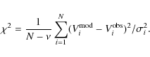
(3)

In our definition of $\chi ^2$ , N is the number of positions with HI column density along the line of sight greater than $5\times 10^{19}$ cm^-2 (N=31391) and $\nu$ is the number of degrees of freedom. It is unreasonable to consider 110 free rings i.e. each ring with 6 degrees of freedom, not only because of the large amount of computer time required to find a solution but also because solutions with so many degrees of freedom are not very robust (parameter variations for 1 out of 110 rings does not give sensible variations to the $\chi ^2$ ). On the other hand the use of functional forms that describe the 6 free parameters as a function of R, each with 2-3 free parameters, often do not give satisfactory results (e.g. Corbelli & Schneider 1997). Following Corbelli & Schneider (1997) we constructed a model in which the properties of 11 equally spaced rings could be varied independently. We shall call these the ``free rings''. The first free ring is centered at 10 kpc, the last one at 35 kpc. This is because placing the first/last free ring at smaller/larger galactocentric distance make them not very stable. We extrapolate the geometrical parameters of the first/last free ring for 2 kpc inward/outward when using the tilted ring model to derive the rotation curve at radii between 8 and 37 kpc. The parameters of the 10 rings between 2 free rings are found by linear interpolation. Our procedure is to search for a minimum $\chi ^2$ value considering the parameters of the 110 rings.

Given the numerous free parameters ( $\nu=66$ ) it is still unreasonable to search for the minimal solution scanning a multidimensional grid (of 66 dimensions). We use two procedures to determine the best fitting model. In the first procedure (hereafter P1) we apply the technique of partial minima. We evaluate $\chi ^2$ by varying each parameter separately and interpolating to estimate the value for a minimum $\chi ^2$ for each parameter. We then repeat the procedure over a smaller parameter interval around the new solution. We start the minimization with the following initial set of free parameters: $i=77^\circ$ , $\theta=38^\circ$ , $V_{\rm sys}=-300$ km s^-1, $\Delta x_{\rm c}=\Delta y_{\rm c}= 0$ for all free rings. As an initial guess of $V_{\rm c}$ we give the average rotational velocity derived in each free ring by deprojecting the observed velocities within a 20 $^\circ$ cone of the optical line of nodes, $\theta=38^\circ$ (using $i=77^\circ$ and $\theta=38^\circ$ for the deprojection). We carried out several optimization attempts under a variety of initial conditions to avoid that our partial minima technique carries the solution towards a relative minimum.

The best fitting ring model is shown in Figure 2 by the heavy continuous line. It gives a $\chi^2=2.18$ . We display only 3 of the 6 free parameters for each free ring, namely the inclination i, the position angle $\theta$ and the systemic velocity $V_{\rm sys}$ . The shifts of the orbital centers are small and shown in Fig. 5. The minimum $\chi ^2$ is obtained for an inclination which radially decreases by a few degrees between 10 and 25 kpc in radius and then increases out to 85 $^\circ$ for the outermost ring. The position angle shows marginal variations out to 25 kpc, then it decreases by about 10 $^\circ$ in the outskirts. However, while from 10 to 28 kpc low $\chi ^2$ values are obtained for combinations of i and $\theta$ not very different than the best fitting model, beyond 28 kpc we can find tilted ring models which give acceptable fits (with a $\chi ^2$ value within 20 $\%$ of the minimum) with different combinations of i and $\theta$ . The short dashed line in Fig. 2 shows one model for which the inclination of the outermost rings does not increase and their position angle instead varies between 30 $^\circ$ and 45 $^\circ$ . Clearly the outermost rings are not very stable, due to a lack of 21-cm emission at these large radii. Hence, some care is required when the model is extrapolated to even larger radii. The single constant value of systemic velocity which minimizes the $\chi ^2$ is -306 km s^-1. The errorbars displayed for the best fitting model indicate parameter variations for which the $\chi ^2$ of the model is within 20 $\%$ of the minimum. This is done varying just one parameter at a time with respect to the combination of parameters which gives the minimum $\chi ^2$ . The rotational velocities $V_{\rm c}$ obtained from the fit will be discussed in the next Section where we compare them to the rotation curve of Andromeda derived from the first moment map using the geometrical parameters and $V_{\rm sys}$ of the best tilted ring model.

$\begin{figure} \par\includegraphics[width=8.5cm,clip]{13297f02.eps} \end{figure}$

Figure 2:

Assortment of ``free ring'' models fit to the HI data according to modeling procedure P1. We display 33 of the 66 free parameters: the inclination i, position angle $\theta$ and systemic velocity $V_{\rm sys}$ of the 11 free rings. The heavier continuous lines show the best fitting model which gives the minimum $\chi ^2$ solution (circled points). For this case we vary one parameter of a given ring keeping all others at the best fitting values. Dashed lines indicate some other combinations of free parameters which give a $\chi ^2$ within within 20 $\%$ of the minimum value.

Open with DEXTER

In a second procedure (hereafter P2) we searched for a minimum by neglecting the radial variations of $V_{\rm sys},x_{\rm c},y_{\rm c}$ . We set $\Delta x_{\rm c}=\Delta y_{\rm c}= 0$ and $V_{\rm sys}=-306$ km s^-1. We have determined this value of $V_{\rm sys}$ as described below. In M 31, the integrated 21-cm profile shows that the North-East receding side has more gas than the South-West approaching side (their ratio being 1.13), at intermediate velocities between the central one and the velocity of maximum emission. This is likely due to the disturbance caused by interaction with M 32. Hence we cannot simply compute the systemic velocity by averaging the observed mean velocities and weighting these with the 21-cm surface brightness. Considering the galaxy disk between 10 and 25 kpc with an average inclination of 77.7 $^\circ$ and position angle 38 $^\circ$ we compute the average systemic velocity in rings. We weight the data with the surface brightness intensity. For points south of the minor axis we multiply their weight by the ratio of the HI mass in the northern side to that of the southern side in that the ring. The resulting $V_{\rm sys}$ is shown in Fig. 3. Averaging the systemic velocities over all rings we thus obtain a value of -306 km s^-1. We searched for a minimal solution scanning a multidimensional grid (12 dimensions) corresponding to parameter variations of the outermost 4 free rings. The initial grid of variations for the inclination and position angle considered are $\pm$ $15^\circ, \pm 10^\circ$ , $\pm$ $5^\circ$ around the standard values of the inner disk ( $i=77.6^\circ$ , $\theta=38^\circ$ ). The maximum velocity shifts considered with respect to the initial values of $V_{\rm c}$ are $\pm$ 25,15,10,5 km s^-1. We then consider finer grids for the outermost 4 rings. We have compared the observed velocities to the velocities predicted by tilted ring models using all possible combinations of parameters for the outermost 4 free rings. For the 8 innermost free rings, parameter variations have been consider only in a 3-dimensional space, namely the minimum $\chi ^2$ has been found for one ring at a time, considering all combinations of $i,\theta,V_{\rm c}$ for that particular ring. As shown in Fig. 3 the resulting free parameters for the best fitting tilted ring model are very similar to those obtained using the first method.

$\begin{figure} \par\includegraphics[width=8.5cm,clip]{13297f03.eps} \end{figure}$

Figure 3:

Best fitting P2 solution for i and $\theta$ obtained when $V_{\rm sys}=-306$ km s^-1, $\Delta x_{\rm c} =0$ , $\Delta y_{\rm c} =0$ . All combinations of the 12 free parameters for the outermost 4 free rings have been considered. For the innermost 7 free rings instead the minimum values have been obtained by varying parameters of one ring at a time. Errorbars indicate parameter variations for which the $\chi ^2$ value of the model is within 20 $\%$ of the minimum. The lower panel shows the values of $V_{\rm sys}$ determined by the first order moment map (see text for details) between 9 and 25 kpc, whose average value is -306 km s^-1.

Open with DEXTER

We define the residual velocities as

$\begin{displaymath}{\rm res}=V_{\rm mod}-V_{\rm obs} \end{displaymath}$

(4)

where $V_{\rm mod}$ are the circular velocities $V_{\rm c}$ , as parameterized in the tilted ring model, projected along the line of sight and convolved with the beam function. The observed velocities $V_{\rm obs}$ are the mean velocities detected along the line of sight.

Residual velocities are generally smaller than 10 km s^-1 and no characteristic patterns are visible across the galaxy. It is worth noticing that, if we trace the major axis position angle by a close inspection of the first moment map, the position angle seems about constant at $\sim$ 38 $^\circ$ out to galactocentric distances of 28 kpc, then it decreases to about 32 $^\circ$ at 32 kpc and finally it increases again back to 38 $^\circ$ at 38 kpc. Given the consistency between the best fitting model for the first and second procedure (Figs. 2 and 3) and also between these tilted ring models and the inspection of the database, we will not consider models in which the position angle increases much above 38 $^\circ$ for the outermost rings in the rest of this paper.

2.1 The NEMO results

To check our results for the best fitting tilted ring model we also used the standard least-square fitting technique developed by Begeman (1987), as implemented in the ROTCUR task within the NEMO software package (Teuben 1995) (hereafter P3). The galactic disk is subdivided into rings, each of which is described by the usual 6 parameters. Starting with the initial estimate for the fitting parameters, these are then adjusted iteratively for each ring independently until convergence is achieved. We run NEMO considering or neglecting the variations of the orbital centers and systemic velocity for each ring. The ROTCUR task gives less accurate results than our P1 method since it does not take into account the distance variations between the observer and the far/near side of the galaxy and minimizes the free parameters of one ring at a time without subsequent iterations. We ran ROTCUR with 24 free rings from 8 to 34 kpc. For the last ring the solutions did not converge. We show in Fig. 4 the resulting i, $\theta$ and $V_{\rm sys}$ for 3 cases. In one case the fit is done over all data points with uniform weight, while varying $V_{\rm sys}$ and the orbital centers $x_{\rm c}$ and $y_{\rm c}$ . In a second attempt, we fitted the data weighted with the cosine function of the galactic angle away from the major axis and excluding data within a 20 $^\circ$ angle around minor axis. In a third attempt, we fitted the data without considering possible orbital center shifts and setting $V_{\rm sys}$ to the average value found by ROTCUR when $V_{\rm sys}$ was allowed to vary. This method confirms that the average systemic velocity of the disk of Andromeda is slightly more negative than previously thought and that there is a warp in outer disk which brings the orbits closer to be edge-on.

We conclude that the 3 fitting methods largely produce similar results and will make use of the results of most accurate procedure, P1, in the rest of the paper.

$\begin{figure} \par\includegraphics[width=8.5cm,clip]{13297f04.eps} \end{figure}$

Figure 4:

Best fitting solutions obtained with the task ROTCUR in the NEMO package (P3). The resulting position shifts of orbital centers are very small and hence are not shown. The open circles indicate the best fitting parameters when we exclude data within a 20 $^\circ$ angle around minor axis in the plane of the galaxy and the data is weighted into the least squares solution with the cosine of the galactic angle away from the major axis. The triangles indicates the solution computed for all data (including points along minor axis) and for uniform weight. The star symbols show the best fitting solution obtained by keeping the orbital centers fixed, and the systemic velocity equal to -305 km s^-1, the average value obtained when we allow it to vary radially.

Open with DEXTER

$\begin{figure} \par\includegraphics[width=8.5cm,clip]{13297f05.eps} \end{figure}$

Figure 5:

Orbital center shifts in arcmin as derived from tilted ring model fits. Positive values of $\Delta x_{\rm c}$ correspond to orbital centers shifted towards decreasing RA values with respect to 10.6846853 $^\circ$ which is Andromeda's center. Positive values of $\Delta y_{\rm c}$ correspond to orbital centers shifted towards increasing Dec values with respect to the central value of 41.2690374 $^\circ$ . In panels a) and b) we show the values corresponding to tilted ring models P1 in Figure 2 where we have considered these variables. Similarly in panels c) and d) the values derived for models P3 shown in Fig. 4.

Open with DEXTER

2.2 Comparison with previous results

As we mentioned in the Introduction, only recently a 21-cm survey made with a synthesis telescope has been used to model the warp and the rotation curve of M 31 simultaneously (Chemin et al. 2009). The conclusion is similar to ours, namely that the warp of M 31 is such that the outer disk is at higher inclination and lower position angle than the inner disk. However a close inspection reveals some differences. First, the average value of the disk inclination between 6 and 27 kpc that Chemin et al. (2009) find is 74 $^\circ$ while what we find between 10 and 28 kpc is 77 $^\circ$ , more consistent with that derived from optical surface photometry Walterbos & Kennicutt (1987). Secondly, the inclination of the outermost fitted radius is higher for our model compared to what Chemin et al. (2009) find, while the position angle is slightly lower. We list below three main differences in the two fitting methods which can help explaining the variations in the resulting tilted ring model parameters.

- We model the bulk rotational velocity of M 31 using the mean rotational velocity observed at each position. That is, we use the first moment map made from the 120 arcsec by 2 km s^-1 data cube, following 4- $\sigma$ blanking in the 120 arcsec by 18.5 km s^-1 data cube to determine what is included in the integral. Chemin et al. (2009) use the peak velocity and if there are multiple components they use the peak velocity of the ``main component''. The main component is defined to be the one which has the largest velocity relative to the systemic velocity of the galaxy. Their choice is based on the observational evidence of multiple peak profiles, very prominent in the inner regions. As we explain fully in the next subsection we did not include the innermost region (from 0 to 8 kpc in radius) in our analysis because it is dominated by non-circular motions. Even though taking the mean velocity we might be systematically biased to lower apparent rotational velocities, the bias effects are minimal at large radii where we are most interested to the dynamics. In general, we find that assuming the peak velocity of the main component as the best approximation to the rotation curve, as in Chemin et al. (2009), is very model dependent. Moreover, to determine it in a robust way one has to assume certain observational conditions (i.e. to which level is a high velocity feature accepted in terms of signal-to-noise; also, what happens if the highest velocity feature is blended inside a bright component so that only a ``shoulder'' but not a secondary peak can be seen in the spectra). Even though it is true that observations carried out with a low resolution and projection effects bias the mean velocity towards lower velocities, we feel that results might be more robust when considering the mean velocity than other estimates if the system is as complex, asymmetric and disordered as M 31 (and observed with a high spatial resolution). Accretion events, which M 31 is experiencing, produce several distinctive morphological and dynamical signatures in the disk, including long-lived ring-like features, significant flares, bars and faint filamentary structures above the disk plane. In M 31, the likely non-negligible disk thickness coupled with a complex, asymmetric warping and with the presence of non-circular motion related to multiple spiral arm segments intersecting along the line of sight, makes difficult to assess the reliability of velocity indicators different than the mean for tracing the bulk circular motion of the disk. To prove the complexity of the system, we would like to point out that across the disk of M 31 and especially along the bright ring-like structure at 10-15 kpc in radius, double peak profiles are often present. Sometime peaks are separated by more than 100 km s^-1. There is however not a systematic azimuthal or radial pattern as to whether is the fainter or the brighter peak to show the most extreme velocity from systemic. If it is just the warped outer disk superimposed with the main disk to cause the multiple peak profiles we should have found a more systematic behavior since the neutral hydrogen surface density decreases considerably beyond 15 kpc. High resolution IR maps of M 31 (Gordon et al. 2006) show that the northern half the 15 kpc arm, distinct on the major axis, merges into other spiral arms (or ring like structure) at 10 kpc. Peak velocities might more closely trace non-circular motion of the arms and produce wiggles in the rotation curve which do not average out when additional perturbations are present. This is the case for M 31, in which the southern half is more strongly tidally perturbed than the northern half. Such a curve cannot be reproduced without modelling the spiral arms locally in term of mass condensation and non-circular motion.

- As we mentioned earlier in this section we believe that it is relevant for M 31, a very extended and nearby galaxy, to derive galactocentric distances in the frame of a tilted ring model using appropriate spherical geometry. This takes into account the fact that the near side of the galaxy is effectively closer than the far side of the galaxy. Procedures often available for deriving the kinematical parameters are built for the more numerous more distant galaxies and do not account for this effect. Moreover, our routine works with 66 free parameters simultaneously since the best fitting values of the parameters for each ring cannot be found independently from those relative to other rings when a warp is present. In fact the warp makes two or more rings overlap along the line of sight and in the overlapping region the expected velocity depend on all parameters of the rings which overlap.

- In fitting the tilted ring model to the data we do not apply any angular dependent weight i.e. the same weight is given to pixels close to minor axis than to major axis. This is because we would like to minimize the risk of amplifying the kinematical signatures of sporadic features which happens to lie close to major axis. As we will see in the next Section, our model produces a stable rotation curve, not very sensitive to the choice of the opening angle $\alpha_{\rm max}$ around the major axis.

2.3 Why exclude the innermost region from fitting

Opposite to Chemin et al. (2009) we do not include the inner regions in our analysis. This is because after the pioneer work of Lindblad (1956) several other papers have pointed out in the inner region of M 31 the presence of morphological structures, such as a bar and a bulge, associated with streaming motion and non-circular orbits (e.g. Beaton et al. 2007; Athanassoula & Beaton 2006; Gordon et al. 2006; Stark & Binney 1994). In particular Berman & Loinard (2002); Berman (2001) have shown that the anomalous velocities observed in the inner region of M 31 can be explained as the response of the gas to the potential of a triaxial rotating bulge. Using a bulge effective radius of 10 arcmin they have derived which family of periodic elliptical orbits exist. They find that the bulge gives a non-negligible contribution to the galaxy potential out to about 7 kpc, and only at larger radii circular motion related to the disk gravitational potential dominates. The model well reproduced the velocities observed through the CO J=1-0 line emission. Since in this paper we are only modelling the large scale circular motion of the disk we use the mean velocity of the HI gas as tracer of the circular velocity from 8 kpc outwards.

$\begin{figure} \par\includegraphics[width=8cm,clip]{13297f06.eps} \end{figure}$	Figure 6: Rotational velocities derived for the northern and southern halves of M 31 using the geometrical parameters of the best fitting tilted ring model as shown in Fig. 2. For this figure $\alpha _{\rm max}=30^\circ$ . The filled circles indicate the best fit rotational velocity parameters derived by the tilted ring model fit P1.
Open with DEXTER

3 The rotation curve and the radial distribution of the baryons

We now apply the geometrical parameters of the best fitting tilted ring model to derive the rotation curve of the galaxy. We set the inclination, position angle and systemic velocity to the values shown by the heavy continuous line in Fig. 2, and consider also the small shifts of the orbital centers obtained by our minimization procedure P1. We derive the rotation curve by averaging the rotational velocities of data points in radial bins 1 kpc wide. For radii between 8 and 10 kpc, we extrapolate the model parameters of the innermost ring centered at 10 kpc. For radii larger than 35 kpc, we extrapolate the model parameters of the outermost ring at 35 kpc. Just for curiosity, we also checked what would be the rotation curve of the inner regions for our dataset if we assume circular motion and inside 8 kpc we set the disk inclination equal to the inclination of the ring at 10 kpc and we consider 28 $^\circ$ as position angle (this is the average value we derive from an inspection of the mom-1 map). For this innermost region we consider zero shifts for the orbit centers and -306 km s^-1 as systemic velocity. Figures 6 and 7 show the large dispersion in the velocities relative the central region due to the presence of multiple components and to the uncertainties related to orbital eccentricities inside 8 kpc, discussed in the previous section. To complement 21-cm data in the inner regions we show in Fig. 7 the peak brightness velocities of CO lines (Loinard et al. 1995). These have been observed along the major axis assumed to be at PA = 38 $^\circ$ and with $i=77^\circ$ . However, notice that this is shown not just to point out the consistency of the molecular and atomic gas velocities, but to emphasize one has to consider non-circular motion to properly trace the rotation curve in the inner region (Berman & Loinard 2002; Berman 2001). Hence we shall not use the CO data as well as the 21-cm data at radii smaller than 8 kpc. In the rest of the paper, we will only analyze the rotation curve between 8 and 37 kpc. Beyond 37 kpc the northern and southern halves do not give consistent rotation curves for any of the deconvolution models. This is likely due to highly perturbed orbits in the outermost regions, especially for the southern half which is closer to M 32.

$\begin{figure} \par\includegraphics[width=8cm,clip]{13297f07.eps} \vspace*{-4mm} \end{figure}$

Figure 7:

The bottom panel shows the rotation curves obtained for the northern and southern halves of the galaxy by averaging the data shown in Fig. 6 in radial bins 1 kpc wide. Errorbars refer to the dispersion around the mean. Filled triangles are for the northern half, open squares for the southern half of the galaxy. Rotational velocities in the inner region derived from CO data by Loinard et al. (1995) are shown with filled and open circles for the northern and southern major axis, assumed to be at PA = 38 $^\circ$ and with $i=77^\circ$ . The filled dots in the upper panel show the global rotation curve. As explained in the text, errorbars take into account the dispersion around the mean and the differences between the values for the two halves of the galaxy. The vertical dashed line mark the innermost radius which will be considered in this paper for the dynamical analysis.

Open with DEXTER

We consider points which lie within an opening angle $\alpha_{\rm max}$ on either side of the major axis. We first derive the rotation curve in the northern and southern halves separately. We check the consistency of the rotation curves for different values of $\alpha_{\rm max}$ , with the value of the rotational velocities determined by the tilted ring model over the whole galaxy, and between the northern and the southern halves. When we vary $\alpha_{\rm max}$ between 15 $^\circ$ and 75 $^\circ$ , we obtain the same rotation curves consistently (variations are less than 1 km s^-1). Only the dispersion around the mean increases slightly as we increase $\alpha_{\rm max}$ . We shall use $\alpha _{\rm max}=30^\circ$ for the rest of the paper. The rotation velocities in the two halves are consistent (within 3- $\sigma$ ). At many radii, mean velocities in the northern and southern halves differ by less than 1- $\sigma$ corresponding to only a few km s^-1 at most, as shown in Figs. 6 and 7. In Fig. 6 we also display the rotational velocity parameter of the best tilted ring model. The best fitting ring model gives the most consistent rotation curves. We also tried to deconvolve the observed velocities using other tilted ring models shown in Fig. 2, but they give less consistent rotation curves. Average velocities are derived in the two halves by assigning a weight to each pixel equal to the integrated brightness intensity i.e. to the HI column density along the line of sight in the limit of optically thin 21-cm line. The global rotation curve is the arithmetic mean of the average rotational velocities in the two galaxy halves. The errorbars of the global rotation curve shown in the upper panel of Fig. 7 are computed as

$\begin{displaymath}\sigma_g={V_{\rm hi}-V_{\rm low} \over 2} + {\sigma_{\rm hi}+\sigma_{\rm low}\over 2} \end{displaymath}$

(5)

where $V_{\rm hi}$ refers to the highest rotational velocity and $V_{\rm low}$ to the lowest rotational velocity between the two mean velocities relative to the northern and to the southern galaxy side; $\sigma_{\rm hi}$ and $\sigma_{\rm low}$ refer to the relative dispersions around the mean.

In Table 1 we give the parameters of the best fitting tilted ring model and of the average rotation curve of M 31 in the radial interval which will be used in the next Section for the dynamical mass model. The position shifts of the orbital centers are rather small and can be neglected. The systemic velocity shifts, $\Delta V_{\rm sys}$ , are computed respect to the nominal value $V_{\rm sys}=-300$ km s^-1.

Table 1: The HI rotation curve of M 31 and the parameters of the best fitting tilted ring model.

3.1 A comparison with other rotation curve measures

In Fig. 8 we show for comparison the rotation curves derived in this paper (continuous line) and some previously determined ones. In panel (a) we display data for north-east galaxy side, in panel (b) for the south-west side and in panel (c) the average values. Original data in (a) and (b) have been scaled according to an assumed distance D=785 kpc and systemic velocity $V_{\rm sys}=-306$ km s^-1. We show both optical data from Kent (1989a) and 21-cm data from Newton & Emerson (1977); Emerson (1976). Unfortunately most of the previous determinations rely on an assumed fixed inclination for the disk and on data along the major axis alone. That implies that possible local velocity perturbations will not be averaged out. These are clearly visible especially in the literature data between 8 and 20 kpc relative to the south-west galaxy half (panel (b)), strongly perturbed by the M 32 tidal interaction. In the northern side we derive a somewhat lower rotational velocity, perhaps due to the presence of the warp which implies a higher disk inclination, not accounted for by previous data analysis. Taking into account these limitations, the general agreement seems good. The asterisk symbols are used in (c) to display the average rotation curve of Chemin et al. (2009) which lies above ours, due especially to somewhat lower inclination the authors derive for the tilted ring model. Also, despite their analysis masking some perturbations such as the external arm, their curve is less smooth than ours. As discussed already in the previous section, this might be due to different choices of velocity components to extract the rotation curve or to their use of weighting function which gives more weight to data points close to major axis. A side effect of this choice is to retain any local velocity perturbation present along major axis.

A position velocity plot made along the photometric major axis, at a position angle of 38 $^\circ$ , is shown in Fig. 9. Our adopted average rotation curve, projected back along major axis, has been superimposed to it (diamonds). The average value of the disk inclination and systemic velocity, as derived in our best fitting tilted ring model in the radial interval of interest, has been used. For a comparison we display also the average rotation curve of Chemin et al. (2009) after applying the disk inclination and systemic velocity corrections adopted by the authors (asterisk symbols). The figure clearly shows that despite the different gas velocities adopted by the two teams to trace the rotation curve, as explained in detail in Sect. 2, differences in the rotational velocities at large radii before deprojection are marginal. The difference between the two measurements becomes more significant when rotation curves (deprojected) are directly compared. This illustrates the relevance of the differences in the parameters of the best tilted ring model found by the two teams. In particular Chemin et al. (2009) derive lower inclination angles for the M 31 disk and hence higher rotational velocities. The agreement between the PV diagram along the major axis and the component of the rotational velocities measured along the line of sight improves, as it should, when using only data in a very small opening angle around the major axis and data in the two galaxy halves are kept separate. Notice, for example, the higher velocity present along the major axis around 0.7 angular offset respect to the average rotation curve. That is also visible in the optical data shown in the middle panel of Fig. 8. This anomalous velocity present along the major axis is averaged out when data from other directions is taken into account.

$\begin{figure} \par\includegraphics[width=8.5cm,clip]{13297f08.eps} \end{figure}$

Figure 8:

The rotation curves derived in this paper (continuous line) and some previously determined ones. In panel a) we display data for north-east galaxy side, in panel b) for the south-west side and in panel c) the average values. Filled circles are for Kent (1989a) optical data along the major axis, open squares and open triangles are for Emerson (1976) and Newton & Emerson (1977) 21-cm data along the major axis. Asterisk symbols are used in c) to display the average rotation curve of Chemin et al. (2009). Original data in a) and b) have been scaled according to an assumed distance D=785 kpc and systemic velocity $V_{\rm sys}=-306$ km s^-1.

Open with DEXTER

$\begin{figure} \par\includegraphics[width=9cm,clip]{13297f09.eps} \end{figure}$

Figure 9:

Position velocity diagram along the photometric major axis, at a position angle of 38 $^\circ$ . A logarithmic scale is used for the brightness and its contours are drawn at 0.013, 0.06, 0.13, 0.6 Jy/beam. The lowest contour is at the 3- $\sigma$ level since $\sigma$ is 4.2 mJy/beam. The continuous line show the rotation curve adopted in this paper while the asterisk trace the rotation curve of Chemin et al. (2009). In both cases, the rotational velocities have been corrected using the average value of the disk inclination and systemic velocity found by the authors in the region shown.

Open with DEXTER

3.2 The bulge-disk decomposition and the stellar distribution

Radial profiles of stellar disk surface brightness can usually be represented by an exponential distribution. The mass-to-light ratio is determined by the dynamical analysis of the rotation curve or by the optical colors once the radial exponential disk scale length is known. The disk scale length can be established from surface brightness profiles in various bands and it might be wavelength dependent. In Andromeda, it varies from 7.7 kpc in the U-band to 5.9 in the R-band (Walterbos & Kennicutt 1988) to 4.5 kpc in the K-band (Hiromoto et al. 1983; Battaner et al. 1986). The images used at optical wavelengths (Walterbos & Kennicutt 1988) can trace the disk surface brightness out to galactocentric radii of about 25 kpc, while the available K-band images (including that obtained through the 2MASS survey) loose sensitivity beyond 20 kpc. The discrepancy between the optical and infrared scalelength can be easily explained in terms of a radially varying star formation history or of an extinction gradient. Light in the K-band traces the mass distribution better than optical light because of the reduced extinction and because most of the stellar mass in galaxy disks is due to old, low mass stars. Therefore for the dynamical analysis, K-band scale lengths are usually preferred despite the reduced sensitivity of infrared images. Recent mid-infrared observations of Andromeda obtained with the Infrared Array Camera on board of the Spitzer Space Telescope (Barmby et al. 2006) show a disk scale length of 6.1 kpc at 3.6 $\mu$ m measured on the same radial interval as measured by Battaner et al. (1986) using the K-band light. A larger scale length at 3.6 $\mu$ m is also found in M 33 by comparing the Spitzer image with the 2MASS K-band image (Verley et al. 2009). This might imply that intermediate age, cool supergiants contribute a substantial fraction of the NIR emission at 3.6 $\mu$ m (Mould et al. 2008).

The determination of the disk scale length depends also on the bulge-disk light decomposition and K-band images might not be deep enough to obtain an accurate bulge-disk decomposition. Nevertheless we feel that the shorter disk scalelength measured in the K-band images compared to 3.6 $\mu$ m images is not affected by this limitation. M 33 in fact has no bulge and indeed the scale length at 2.2 $\mu$ m is shorter than at 3.6 $\mu$ m. A spherical model for the bulge of M 31 is a simplification. Detailed modelling of the surface brightness shows that at very least the bulge is an oblate spheroid with axis ratio of 0.8 (Kent 1983) but most likely it is a triaxial bulge (e.g. Berman 2001, and references therein). For the purpose of this paper, which is the dynamical mass modelling of the disk rotational velocities (beyond 8 kpc), we can neglect the asphericity of the bulge which affects the orbits in the innermost few kpc. Using a R^1/4 de Vaucouleurs law (i.e. a Sersic index of 4) for the light distribution it is customary to characterize the bulge by its effective radius which encloses half of its total light. At optical wavelengths (in the R- and V-band) Walterbos & Kennicutt (1988) found a bulge effective radius of 2.3 kpc and a bulge to disk luminosity ratio B/D = 0.82. Using the same dataset in the R-band combined with Hubble Space Telescope data of Lauer et al. (1993) and data from Kent (1983) for the innermost regions Geehan et al. (2006) derived a much smaller bulge scale radius: 0.61 kpc (similar to what can be inferred by inspecting the 2MASS images). Using the 3.6 $\mu$ m Spitzer image Barmby et al. (2006) modelled the bulge light distribution with a R^1/4 de Vaucouleurs law and found a 1.7 kpc effective radius and a bulge to disk light ratio of B/D = 0.78. Using the same data Seigar et al. (2008) obtain a bulge effective radius of 1.93 kpc for a Sersic index n=1.7, and a disk scalelength of 5.91 kpc with B/D = 0.57. Fits to the bulge light distribution using smaller Sersic indexes have also been done by Worthey et al. (2005) using a brightness profile from an I-band image out to 24 kpc: for a Sersic model with n=1.6 the bulge effective radius was found to be 0.89 kpc and the disk scale length 5.7 kpc, even though a steepening of the scale length is clearly visible beyond 15 kpc. An faint stellar disk which extends as far as 40 kpc from the Andromeda nucleus has been recently pointed out by Ibata et al. (2005) with an exponential scale length of 5.1 kpc in the I-band.

Given the uncertainties in the disk and bulge mass distribution we will attempt to fit the rotation curve using a varying disk scalelength between 4.5 and 6.1 kpc in steps of 0.2 kpc. For the bulge we shall use 4 possible parameter combinations, namely an effective radius of 2.0 and 0.7 kpc and a Sersic index n=4, and n=1.6. Given the fact that we cannot constrain the dynamical contribution of the bulge since we are not fitting the motion in the inner regions, our purpose will be only to see if the dynamical fit to the disk improves considerably when using any of the four combinations.

3.3 Stellar mass-to-light ratios

Analysis of the star formation histories of the bulge and disk of M 31 suggest that there is no age difference between the bulge and the disk (Olsen et al. 2006). However previous attempts to fit former rotation curves of this galaxy found a higher mass-to-light ratio for the disk than for the bulge (Widrow et al. 2003), which was unexpected given the older age of bulges relative to disks. Hydrodynamic simulations of the triaxial bulge of M 31 by Berman (2001) found a B-band mass-to-light ratio of 6.5 for the bulge i.e. a stellar mass of 10¹⁰ $M_\odot$ . In the disk of Andromeda there is also a color gradient visible in the disk (Seigar et al. 2008; Walterbos & Kennicutt 1988) since B-R varies between 1.7 in the inner regions to 1.3 in the outer regions (this can be due to changes in metallicity, age or extinction). According to Bell & de Jong (2001) the mass-to-light ratio in the K-band expected from B-R colors can vary from the value of 1 in the central regions to 0.65 in the outer disk if extinction does not change radially. The mass-to-light ratio in the B-band can vary between 8 and 2.5 $M_\odot/L_\odot$ and we will consider these two values as the extreme acceptable disk mass-to-light ratio values. Since we fit the rotation curve beyond 8 kpc we cannot constrain the bulge mass-to-light ratio and hence we will consider also models with equal mass-to-light ratios for the bulge and the stellar disk.

The bulge and disk blue luminosities which we shall use to compute the mass-to-luminosity ratio are $9\times 10^9$ $L_\odot$ and $2.1\times 10^{10}$ $L_\odot$ respectively. These have been derived using the integrated B-band magnitude measured by Walterbos & Kennicutt (1988), corrected for absorption, assuming that the bulge contribution is 30 $\%$ of the total emission in the B-band. As we mentioned in the previous subsection, the decomposition of the light profile into a bulge and disk component is somewhat uncertain and especially the bulge integrated luminosity is not firmly estabished yet (see also Kent 1989b).

3.4 The gas surface density

For the gaseous disk we shall consider the atomic hydrogen and the molecular gas surface density. These will be multiplied by 1.33 to account for the presence of helium. Using the best fitting tilted ring model (P1) we derive the radial distribution of neutral atomic gas, perpendicular to the galactic plane, in the optically thin approximation. This is shown in Fig. 10 as a function of the galactocentric radius. The corresponding total HI mass is $5.4\times 10^9$ $M_\odot$ . To consider the possible presence of opaque clumps we can multiply the HI surface brightness by 1.3 since this is the correction inferred by Braun et al. (2009). This correction has however no noticeable effect for the dynamical analysis carried out in the next section.

The continuous line in Fig. 10 is the log of the function $f_{\rm HI}(R)$ . We shall use $f_{\rm HI}(R)$ to compute the dynamical contribution of the atomic gas mass to the rotation curve. It has the following expression

$\begin{displaymath}f_{\rm HI}(R) = {\rm e}^{2.3(22.0888-0.08759\ R)\ \exp(-0.11773\ \exp(-0.03276\ R^{1.7}))} \end{displaymath}$

(6)

and it provides a good fit to the atomic surface density distribution perpendicular to the galactic plane. The sharp decline of the HI beyond 27-30 kpc is likely due to the ionization of the atomic hydrogen by the local extragalactic UV background radiation (Corbelli & Salpeter 1993). Hence the fitting function which approximates the total atomic gas distribution is shallower than the HI distribution in the outer region. There is also ionized atomic gas in the inner regions, as can be inferred from the H $\alpha$ emission maps (Walterbos & Braun 1994). However quantifying the column density and the geometrical distribution of such ionized component is subject to several assumptions. The gaseous mass involved is small and irrelevant to the rotation curve fitting since in the inner region it is the stellar component which is dynamically dominant. Hence we shall neglect it.

For the molecular gas fraction we considered the average radial variation (North+South) as shown in Fig. 10 of Nieten et al. (2006).

$\begin{figure} \par\includegraphics[width=9cm,clip]{13297f10.eps} \end{figure}$

Figure 10:

The neutral atomic hydrogen column density perpendicular to the galactic plane is shown as a function of galactocentric distance. The best fitting tilted ring model P1 is used for the deconvolution of the 21-cm line brightness image. The optically thin line approximation has been used to convert the surface brightness in HI gas column density. The continuous line shows the total atomic gas surface density of the M 31 disk as modelled for the dynamical analysis.

Open with DEXTER

4 Dynamical analysis

In this section we will analyze the mass distribution in the Andromeda galaxy. We first attempt to fit the rotation curve of Andromeda, derived in the previous section, from 8 to 37 kpc without a dark matter halo. Then we carry on the dynamical analysis considering two different models for the radial distribution of the dark matter density distribution. We will discuss at the end the resulting total mass of Andromeda in the context also of data at very large radii from observations of the Andromeda satellites and other objects. We shall consider both models in which the the disk and the bulge have the same mass-to-light ratio and models in which these are two independent variables. Unless stated differently we shall consider the HI gas in the optically thin approximation. The half thickness of the disk is assumed to be 0.5 kpc and the contribution of the disk mass components to the rotation curve is computed according to Casertano (1983). We use the reduced chi-square statistic, $\chi ^2$ , to judge the goodness of a model fit. We consider first 2 free parameters: the disk and the bulge mass-to-light ratio (M/L)_d,b, which we vary continuously. For the stellar disk we vary the exponential scalelength h_d using steps of 0.2 kpc in the interval $4.5\le h_d \le 6.1$ kpc. For the bulge we consider 2 possible effective radii h_b and Sersic index n=4 and n=1.7.

4.1 Newtonian and non-Newtonian dynamics without dark matter

We first attempt to fit the rotation curve in the framework of Newtonian dynamics without considering a dark matter halo. The best fit is obtained for a disk scalelength of 6.1 kpc with $(M/L)_d=(M/L)_b=8.0 ~ M_\odot/L_\odot$ , which is the maximum allowed value. The fit is slightly better when a bulge effective radius of 2 kpc is used. This is shown in the top panel of Fig. 11. However the fit is generally poor being the reduced $\chi^2>6$ for all possible combinations of parameters (see Table 2). Hence the model with no dark matter fails to fit the data under the assumption of Newtonian gravity. The fit stays poor even if unreasonably high values for the stellar mass-to-light ratio are considered (> $8 ~ M_\odot/L_\odot$ ). The evident failure is due to the declining rotation curve predicted by the baryonic mass distribution beyond 26 kpc.

An alternative explanation for the mass discrepancy has been proposed by Milgrom by means of the modified Newtonian dynamics or MOND (Milgrom 1983). Outside the bulk of the mass distribution, MOND predicts a much slower decrease of the (effective) gravitational potential, with respect to the Newtonian case. This is often sufficient to explain the observed non-keplerian behavior of RCs (Sanders & McGaugh 2002). According to this theory the dynamics becomes non-Newtonian below a limiting acceleration value, ${a_0}\sim 10^{-8}$ cm s^-2, where the effective gravitational acceleration takes the value $g = g_n/\mu(x)$ , with g_n the acceleration in Newtonian dynamics and x=g/a₀. Here we shall use the critical acceleration value a₀ derived from the analysis of a sample of rotation curves $a_0 = 1.2\times 10^{-8}$ cm s^-2 (Sanders & McGaugh 2002). We have tested MOND for different choices of the interpolating function $\mu(x)$ (see Famaey & Binney 2005, for details). In particular we have used the ``standard'' and the ``simple'' interpolation function and found that the ``simple'' interpolation function provides slightly better fits to the M 31 data. Hence we shall use the ``simple'' interpolating function $\mu(x)=x/(1+x)$ in the rest of the paper.

Corbelli & Salucci (2007) have already tested the former M 31 rotation curve in the MOND framework. They concluded that, in M 31, MOND fails to fit the falling part of the rotation curve at intermediate radii. However, this assessment was made using lower quality data and in the absence of an appropriate knowledge of the tilted ring model parameters.

$\begin{figure} \par\includegraphics[width=84mm,clip]{13297f11.eps} \end{figure}$

Figure 11:

The 21-cm rotation curve for M 31 and the best fitting mass model with no dark halo in the Newtonian case ( top panel) and for MOND ( middle panel). The short-dashed lines indicate the Newtonian stellar bulge and disc contribution to the rotation curve. The dot-dashed line is the gas contribution. The figure displays the the best fitting mass model which is obtained for the Newtonian case when $(M/L)_d=(M/L)_b=8.0 ~ M_\odot/L_\odot$ , h_d = 6.1 kpc, h_b = 2.0 kpc and n=1.6. The MOND best fit ( $\chi ^2=1.3$ ) is obtained when the free parameters are h_d=4.5 kpc, $(M/L)_d=2.5 ~ M_\odot/L_\odot$ $(M/L)_b=5.2 ~ M_\odot/L_\odot$ , and h_b=2 kpc, n=1.6. For comparison we show in the bottom panel the MOND best fit when the disk scalelength h_d is 6.1 kpc. The reduced $\chi ^2$ in this case is higher ( $\chi ^2=3.1$ ), $(M/L)_d=4.1 ~ M_\odot/L_\odot$ , and $(M/L)_b=3.1 ~ M_\odot/L_\odot$ .

Open with DEXTER

Figure 11 shows the MOND best-fit model curve when (M/L)_d and (M/L)_b are two independent free parameters (bottom panel). The mass-to-light ratio best fitting values are (M/L)_d = 2.5, (M/L)_b= 5.2, and h_d = 4.5 kpc. The value of $\chi ^2$ is 1.3, hence MOND provide a good fit to the data. If we reduce the number of free parameters to just one by setting (M/L)_d = (M/L)_b the fit is still reasonably good: the lowest $\chi ^2$ is 1.37 corresponding to $(M/L)_d=(M/L)_b=3.3 ~ M_\odot/L_\odot$ . The rotational velocities predicted by MOND are only slightly higher than observed for $20\le R\le 30$ kpc and slightly lower than the data for $10\le R\le 20$ kpc. As shown in Table 2, the goodness of the fits are not very sensible to the bulge mass-to-light ratio, since we are excluding the central regions. It is however to be noticed that MOND best fits to the actual data require a higher mass-to-light ratio for the bulge than for the disk, in agreement with the expected older age of the bulge stellar component. In M 31 it is around 10 kpc that $g_n\sim a_0$ and non-Newtonian corrections start to be important and force a falling Newtonian RC into a flat one, more consistent with the data. We notice that for MOND the value of the disk scalelength used to fit the baryonic matter distribution is very important. In fact the fit becomes poor if h_d=6.1 kpc, as shown in Fig. 11. If future photometric studies will confirm a disk scalelength of 6.1 kpc then one will have to consider possible variations of the assumed distance to M 31 to make MOND predictions more consistent with the kinematics traced by 21-cm data.

4.2 Dark matter halo models

In the previous subsection we have seen that Newtonian dynamic fits to the rotation curve without considering a dark matter halo are rather poor. We will now use the M 31 rotation curve presented in this paper to test in detail the consistency of a possible halo density profile with theoretical models which predict a well defined dark matter distribution around galaxies. Namely, we shall consider a spherical halo with a dark matter density profile as originally derived by Navarro et al. (1996,1997) for galaxies forming in a Cold Dark Matter scenario. We consider also the Burkert dark matter density profile (Burkert 1995) since this successfully fitted the rotation curve of dark matter dominated dwarf galaxies (e.g. Gentile et al. 2007, and references therein). Both models can describe the dark matter halo density profile using two parameters. The density profile proposed by Burkert (1995) has a constant-density core and is given by:

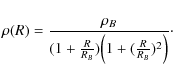
$\begin{displaymath}\rho(R)={\rho_B\over (1+{R\over R_B})\Bigl(1+({R\over R_B})^2\Bigr)} \cdot \end{displaymath}$

(7)

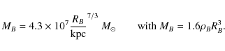
A strong correlation between the two parameters $\rho_B$ and R_B has been found by fitting the rotation curve of low mass disk galaxies (Salucci & Burkert 2000), namely

$\begin{displaymath}M_B=4.3\times 10^7 {R_B\over {\hbox{kpc}}}^{7/3}~ M_\odot \qquad {\hbox{with }} M_B=1.6\rho_B R_B^3 . \end{displaymath}$

(8)

Using this relation, we show in Fig. 12 the best fitting mass model when a Burkert model for the dark halo is considered. The values of the free parameters are: R_B=77 kpc, (M/L)_d=8.0 $M_\odot$ / $L_\odot$ and h_d=5.1 kpc. The reduced $\chi ^2$ value is close to unity, $\chi ^2=0.81$ , meaning the fit is generally good. The best fit $\chi ^2$ does not depend much on the assumed bulge parameters. Even considering (M/L)_d=(M/L)_b the halo model provides an excellent fit to the data. We define the virial mass, $M_{B}^{\rm vir}$ , in the case of a Burkert halo as the mass enclosed in the sphere which has the average dark matter density equal to 98 $\rho_{\rm cr}$ where the critical density for closure is $\rho_{cr}=3 H_0^2/8\pi G$ with H₀=71 km s^-1. The virial mass of the dark halo for best fitting mass model is uncomfortably high: $M_{B}^{\rm vir}=1.2\times 10^{13}$ $M_\odot$ . A Burkert halo which fits M 31 is indistinguishable from a constant density dark matter model since even at the outermost fitted radius, the dark matter density does not decline yet as an R^-2 or R^-3 power law. If we consider core radii smaller than the best fitting value, comparable to the extent of the HI disk, Burkert halo models still provides acceptable fits to the data and implies lower virial masses. In Fig. 13 we show the 68 $\%$ and 95.4 $\%$ confidence areas in the (M/L)_d-R_B plane. For $22\le R_B \le 37$ kpc we have virial masses $8.3\times 10^{11}\le M_{B}^{\rm vir}\le 2.5\times 10^{12}$ $M_\odot$ and $\chi ^2$ values in the 95.4 $\%$ confidence area ( $\chi ^2$ increases as R_B decreases). In the bottom panel of Fig. 12 we show, as an example, a similar mass model to that shown in the top panel, except for the value of the core radius which we set equal to 28 kpc. With such low value of R_Bthe Burkert halo model has a virial mass of $M_B^{\rm vir}=1.4\times 10^{12}$ $M_\odot$ and provides still an acceptable fit to the data ( $\chi ^2=1.17$ ).

$\begin{figure} \par\includegraphics[width=84mm,clip]{13297f12.eps} \end{figure}$

Figure 12:

The M 31 rotation curve (points) and the best-fitting mass models (solid line) using a Burkert dark halo profile with h_d=5.1 kpc, h_b=2 kpc and n=4. Also shown are the dark halo contribution (dot-dashed line), the stellar disk and bulge (short-dashed line) and the gas contribution (long-dashed line). In the top panel, we show the best fit mass model ( $\chi ^2=0.81$ ) with (M/L)_b=4.5 $M_\odot$ / $L_\odot$ , (M/L)_d=8.0 $M_\odot$ / $L_\odot$ and R_B=77 kpc. The case shown in the bottom panel refers to a fixed, lower value of the core radius, namely R_B=28 kpc. For this case the best fitting values of the mass-to-light ratios are (M/L)_b=4.9 $M_\odot$ / $L_\odot$ and (M/L)_d=7.4 $M_\odot$ / $L_\odot$ ( $\chi ^2=1.17$ ).

Open with DEXTER

$\begin{figure} \par\includegraphics[width=6.4cm,clip]{13297f13.eps} \end{figure}$	Figure 13: The 68 $\%$ (darker regions) and 95.4 $\%$ (lighter regions) confidence areas in the (M/L)_d-R_B plane. Clearly the confidence areas extend even beyond the largest R_B value shown. In panel a) (M/L)_d=(M/L)_b, while in b) (M/L)_d and (M/L)_b are two independent variables.
Open with DEXTER

The NFW density profile is:

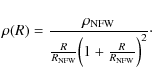
$\begin{displaymath}\rho(R)={\rho_{\rm NFW} \over {R\over R_{\rm NFW}}\Bigl(1+{R\over R_{\rm NFW}}\Bigr)^2} \cdot \end{displaymath}$

(9)

Numerical simulations of galaxy formation find a correlation between $\rho_{\rm NFW}$ and $R_{\rm NFW}$ which depends on the cosmological model (e.g. Avila-Reese et al. 2001; Navarro et al. 1997; Bullock et al. 2001; Eke et al. 2001). Often this correlation is expressed using the concentration parameter $C\equiv R_{\Delta}/R_{\rm NFW}$ and $M_\Delta$ or $V_{\Delta}$ . $R_{\Delta}$ is the radius of a sphere containing a mean density $\Delta$ times the cosmological critical density, $V_{\Delta}$ and $M_\Delta$ are the characteristic velocity and mass inside $R_{\Delta}$ . In this paper we use the results of N-body simulations in $\Lambda$ CDM, cosmology to define the relation between the concentration and the virial mass of dark matter halos. We adopt a flat $\Lambda$ CDM cosmology with parameters from the WMAP results (Spergel et al. 2003), matter density $\Omega_{\rm M}=0.27$ , baryon density $\Omega_b=0.044$ , a normalized Hubble constant $h\equiv H_0/$ (100 km s^-1 Mpc^-1) = 0.71. In this framework, we use the results of the numerical simulation of Macciò et al. (2007), which are in agreement with the results of Neto et al. (2007), and give the following relation between the concentration and the halo mass for relaxed halos:

$\begin{displaymath}C= 7.5 (M_{\Delta}/10^{14} ~h^{-1}~ M_\odot)^{-0.098} \end{displaymath}$

(10)

where $M_\Delta$ is the halo mass for a density contrast $\Delta=98$ . Generally the dispersion in the concentration decreases monotonically as a function of halo mass. The scatter around $\log C$ given by the above relation, is about $\pm$ 0.13 at the expected virial mass of Andromeda (i.e. 10¹² $M_\odot$ ), and a similar value is found for the average total scatter over the mass range considered.

We now fit the M 31 rotation curve using two free parameters: the halo concentration C and (M/L)_d, the disk mass-to-light ratio. We shall consider first no dispersion around the relation given by the above equation and a bulge mass-to-light ratio equal to that of the disk. The 1- $\sigma$ , 2- $\sigma$ and 3- $\sigma$ ranges are determined using the reduced $\chi ^2$ and assuming Gaussian statistics. They are computed by determining in the free parameter space the projection ranges, along each axis, of the hypersurfaces corresponding to the 68.3 $\%$ and 95.4 $\%$ confidence levels.

The best fitting mass model is obtained for a disk scalelength h_d=4.5 kpc. The bulge parameters are not of much relevance for the goodness of the fit in the region of interest to this paper. The stellar mass-to-light ratio for the best fit is (M/L)_d=4.2 $M_\odot$ / $L_\odot$ , if we assume that it does not vary between the bulge and the disk component, and the value of the reduced $\chi ^2$ is 1.12. The total dark halo mass is $M_\Delta=10^{12}$ $M_\odot$ (corresponding to C=11.9). If we allow variations between the disk and the bulge mass-to-light ratio, the best fit mass model gives (M/L)_d=5.0 $M_\odot$ / $L_\odot$ and (M/L)_b=2.7 $M_\odot$ / $L_\odot$ and a minimum $\chi ^2$ value of 1.08. These combination of M/L ratios is not realistic since we don't expect the bulge to have a lower M/L ratio than the disk. But higher values of the bulge M/L ratio increases only slightly the $\chi ^2$ value. In Fig. 14 we show the modelled rotation curve according to the best fitting mass model when h_b=2.0 kpc and n=4. The dark halo mass is $M_\Delta=1.2\times10^{12}$ $M_\odot$ corresponding to C=12. As we increase the disk scalelength the $\chi ^2$ increases slightly, the dark halo mass decreases and the stellar mass-to-light ratio increases (for example for a change in the disk scalelength from 4.5 to 6.1 kpc the minimum $\chi ^2$ changes from 1.12 to 1.34, $M_\Delta$ decreases from $1.2\times 10^{12}$ to $7.5\times 10^{11}$ $M_\odot$ and (M/L)_b,d=5.7 $M_\odot$ / $L_\odot$ ).

$\begin{figure} \par\includegraphics[width=84mm,clip]{13297f14.eps} \end{figure}$

Figure 14:

The M 31 rotation curve (points) and the best-fitting mass model (solid line) using the NFW dark halo profile with C=12 in the frame of $\Lambda CDM$ . Also shown are the dark halo contribution (dot-dashed line), the stellar disk and bulge (short-dashed line) and the gas contribution (long-dashed line). The bottom panel refers to the case ( (M/L)_d=(M/L)_b=4.2 $M_\odot$ / $L_\odot$ ). The top panel refers to the best fit when the mass-to-light ratio of the disk and the bulge are two independent variables. For the best fit (M/L)_d=5.0 and an (M/L)_b=2.7 $M_\odot$ / $L_\odot$ . These combination of M/L ratios is not realistic since we don't expect the bulge to have a lower M/L ratio than the disk. But higher values of the bulge M/L ratio increases only slightly the $\chi ^2$ value and require similar dark matter distribution. Both fits refer to a bulge model with h_b=2.0 kpc and n=4.

Open with DEXTER

We have computed the confidence area in the (M/L)_d-C plane and shown them in Fig. 15. When the mass-to-light ratio of the disk and the bulge are two independent variables the best fitting (M/L)_b value is unrealistically low but the value of the concentration parameters does not change. Figure 15 shows also the wider confidence areas obtained when twice the dispersion of $\pm$ 0.13, as estimated from numerical simulations, is considered around $\log C$ in the $C{-}M_\Delta$ relation.

$\begin{figure} \par\includegraphics[width=84mm,clip]{13297f15.eps} \end{figure}$

Figure 15:

The 68 $\%$ (darker regions) and 95.4 $\%$ (lighter regions) confidence areas in the (M/L)_d-C plane. Panel a) and b) refers to the case where the average $C{-}M_\Delta$ relation is considered with no dispersions around it. In panel a) (M/L)_d=(M/L)_b, while in b) (M/L)_d and (M/L)_b are two independent variables. In panel c) the confidence areas are for the (M/L)_d=(M/L)_b case when 2- $\sigma =0.26$ around the average log C-log $M_\Delta$ relation is considered.

Open with DEXTER

Table 2 summarizes the main results of the mass models considered for fitting the rotation curve of M 31. In Col. (1) we give the short name of the mass model: No-DM is simply a Newtonian dynamic fit with no dark matter. For MOND we use the no dark matter and the ``simple'' interpolation function. The scalelengths of the bulge and of the disc are labeled with the symbol h_b and h_d respectively. We consider h_d as a free parameter in the interval 4.5-6.1 kpc. The best fitting value of a possible additional free parameter of each model, P⁺ is given in Col. (7). For the No-DM and MOND models there is no additional free parameter. For the Burkert halo model P⁺ is the core radius in kpc, for the $\Lambda$ CDM mass model P⁺ is the concentration parameter C. For the bulge and disk mass-to-light ratio, the range of possible values considered are: 2.5 $\le$ (M/L) $_b\le 8.0$ in units of (M/L) $_\odot$ . In the first half of the Table, we consider both (M/L)_b and (M/L)_das free parameters while in the second part we use (M/L)_b = (M/L)_d. Since, for the simple Newtonian dynamic fit with no dark matter, the bulge and disk mass-to-light ratios come out equal to the highest allowed value, the parameters are listed only in the first part of the table.

We can see clearly in Table 2 that the goodness of the fit does not depend on the bulge mass distribution, as expected, since we are only fitting the rotation curve for R>8 kpc. It also shows that only a pure Newtonian mass model with no dark matter halo fails to fit the data. Both MOND, a Burkert halo model with a large constant density core, and the NFW profile in the framework of $\Lambda CDM$ provide good mass model fits to the rotation curve of Andromeda derived in this paper. In the next subsection we shall use data from other sources to test the rotation curve at larger radii than those provided by the HI dataset.

Table 2: Parameters of the best fitting mass model.

4.3 Baryonic and total mass of Andromeda

We consider now the mass estimate of Andromeda from different sources at galactocentric radii from 30 to 560 kpc. We derive a rotation curve by computing the expected circular rotational velocity given the mass estimate within a radius R. We consider data from planetary nebulae, globular clusters, stellar streams and Andromeda satellites to constrain the Andromeda total mass at large radii. Since each paper considers an ensemble of objects and describes in detail the method used to derive the mass, we give in Table 3 the resulting mass estimate and reference the original papers where a more detailed description of the database and analysis can be found. If the authors have assumed a different distance to Andromeda than what we use in this paper, we have scaled their radius and mass estimate accordingly. In Fig. 16 we plot the rotational velocities at large distances from the center of Andromeda derived from the mass estimates given in Table 3.

Table 3: Andromeda mass estimated at large galactocentric radii.

We plot also the velocities at large radii predicted by the $\Lambda CDM$ mass models which best fits our rotation curve i.e. a NFW dark halo profile with concentration C=12 (continuous line). A Burkert halo model with a very large core radius, such as that required by the best fitting mass model to the 21-cm rotation curve data, predicts higher velocities than observed at distances shown in Fig. 16. But a Burkert halo profile with a core radius R_B=28 kpc, compatible with the 21-cm rotation curve data, is also compatible with data at large galactocentric distances (short dashed line in Fig. 16). For both halo models we have considered the values of the free parameters h_d, (M/L)_d and (M/L)_b, which best fit 21-cm rotation curve. Given the fact that the $\Lambda CDM$ and Burkert halo were constrained using only HI data between 8 and 37 kpc it is quite remarkable how well the two halo models fit the data out to about 560 kpc. We did not test MOND predictions in this framework because Andromeda masses in the original paper have been derived using Newtonian dynamic.

Since the best fit Burkert halo model was essentially a constant density profile in the region traced by the 21-cm rotation curve, we show also the predicted velocities of this model in case the dark halo is truncated beyond 37 kpc. A simple keplerian fall off of the observed velocities outside the region covered by our 21-cm dataset however fails to fit the data at larger galactocentric radii. Only the outermost 3 data points are compatible with a keplerian fall-off regime. For the $\Lambda CDM$ mass model, the virial radius corresponding to a concentration C=12 is 270 kpc, hence the predicted rotational velocities of the outermost data points in Fig. 16 are in the keplerian regime.

The best fitting $\Lambda CDM$ mass model implies a stellar (disk+bulge) mass of $1.3\times 10^{11}$ $M_\odot$ and a dark matter halo mass of $1.2\times 10^{12}$ $M_\odot$ . Adding to the stellar mass the cold gas mass (neutral and molecular hydrogen plus helium) of $7.7\times 10^9$ $M_\odot$ we estimate a total baryonic mass of Andromeda of $1.4\times 10^{11}$ $M_\odot$ . This adds to the dark matter halo mass, giving

$\begin{displaymath}M_{\rm tot}=1.3\times 10^{12}~ {{M}}_\odot \end{displaymath}$

(11)

as our best estimate of the total mass of the Andromeda galaxy. The associated baryonic fraction is 0.12, very similar to the cosmic inferred value of 0.14.

$\begin{figure} \par\includegraphics[width=8.5cm,clip]{13297f16.eps} \end{figure}$

Figure 16:

Rotational velocities predicted at large distances from the center of Andromeda according to several datasets analyzed by previous papers (see Table 3 for details). The continuous line shows the rotational velocities predicted by an extrapolation at large radii of the best fitting mass model with a NFW dark halo profile (C=12). The short dashed line shows the predicted velocities of a Burkert halo model with R_B=28 kpc. The long dashed line is for a constant halo dark matter density profile which is truncated outside 37 kpc and gives a Keplerian fall off of the velocity at larger distances.

Open with DEXTER

5 Summary

We determine the rotation curve of the M 31 disk from 8 to 37 kpc using a tilted ring model fit to the velocity field mapped in the full-disk, 21-cm imaging survey of Braun et al. (2009). The orientation of the rings have been determined using three different techniques which give rather similar results. For our most accurate modelling method (P1), we use 11 equally spaced free rings, which cover galactocentric distances between 9 and 36 kpc, whose parameters are varied independently. Each free ring has 6 degrees of freedom, since we allowed the systemic velocity and center position of each ring to vary (in addition to the circular rotation, inclination and position angle). This implies a total of 66 degrees of freedom in our model. Between two consecutive free rings, parameters are determined by a linear interpolation. We find that the disk of M 31 warps from 25 kpc outwards by lowering its position angle and becoming more inclined with respect to our line of sight. The disk reaches an inclination of 86 $^\circ$ at 35 kpc. The geometry of the outermost two rings has somewhat larger uncertainties, but the tilted ring model which gives the best fit to the data also produces consistent rotation curves in the two separate halves of the galaxy. Furthermore, these rotation curves do not depend on the value of limiting angle around the major axis chosen for selecting the data. We find -306 km s^-1 as the average value of the systemic velocity of the gaseous disk of M 31. The rotation curve of M 31 is consistent with being flat beyond 20 kpc and we carry on a dynamical analysis to determine the baryonic and non-baryonic mass distribution of the nearest spiral galaxy.

The M 31 rotation curve cannot be reproduced using Newtonian dynamics and only the stellar and gaseous mass components. Without a dark matter halo however, MOND provide a good fit to the galaxy gravitational potential in the region considered. We test the density profile and mass predictions of hierarchical clustering and structure formation in a $\Lambda$ CDM cosmology, together with a dark halo model having a constant density core. Both models are able to reproduce the rotation curve of M 31 to a high level of accuracy. The constant density core model which fits M 31 has a core radius comparable to the size of the disk of M 31 and therefore is in practice a constant dark matter density model.

Using the relation between the concentration parameter C and the dark halo mass $M_\Delta$ as for a NFW density profile in a flat $\Lambda$ CDM cosmology, we find a best fit halo concentration parameter C=12 which implies a dark matter halo mass $M_\Delta=1.2\times10^{12}$ $M_\odot$ . If we assume that the stellar disk and the bulge have the same mass-to-light ratio we find $(M/L)_d=(M/L)_b=4.2\pm 0.4$ $M_\odot$ / $L_\odot$ . If the mass-to-light ratio of the disk and the bulge are two independent variables then the best fit gives a slightly higher value for the disk, (M/L)_d=5.0^+0.6_-1.0. We are unable to constrain the bulge mass-to-light ratio since we discarded the innermost rotation curve in our fit (derived without considering elliptical orbits). A wider range of C and (M/L)_d values are found when a dispersion is considered around the average log C - log $M_\Delta$ relation, as suggested by numerical simulations of structure formation in a $\Lambda CDM$ cosmology.

An interesting result is that the extrapolation of a constant core dark halo model, as well as of the best fit $\Lambda CDM$ dark halo model, beyond the region traced by the rotation curve are in good agreement with the Andromeda mass traced by other dynamical indicators (globular clusters, streams, satellites) at larger radii, out to 560 kpc. The constant-core best fitting halo model has a very large core radius (77 kpc) and a high virial mass, not consistent with the data at large galactocentric radii. However models with a somewhat smaller core radius, provide acceptable fit to the 21-cm rotation curve and to data at larger galactocentric radii. The total estimated mass of M 31 from our mass model fit to the 21-cm rotation curve in the framework of $\Lambda CDM$ cosmology is 1.3 $^{+0.3}_{-0.3}\times 10^{12}$ $M_\odot$ , with a 0.12 baryonic fraction. This is similar to the cosmic inferred baryonic fraction of 0.14 and implies a formation redshift z_f=1.2 for the Andromeda galaxy.

Acknowledgements

R.W. acknowledges support from Research Corporation for the Advancement of Science. We acknowledge the anonymous referee for his/her criticism to an earlier version of the paper.

References

Athanassoula, E., & Beaton, R. L. 2006, MNRAS, 370, 1499 [NASA ADS] [CrossRef] [Google Scholar]
Avila-Reese, V., Colín, P., Valenzuela, O., D'Onghia, E., & Firmani, C. 2001, ApJ, 559, 516 [NASA ADS] [CrossRef] [Google Scholar]
Babcock, H. W. 1939, Lick Observatory Bulletin, 19, 41 [Google Scholar]
Bajaja, E., & Shane, W. W. 1982, A&AS, 49, 745 [NASA ADS] [Google Scholar]
Barmby, P., Ashby, M. L. N., Bianchi, L., et al. 2006, ApJ, 650, L45 [NASA ADS] [CrossRef] [Google Scholar]
Battaner, E., Beckman, J. E., Mediavilla, E., et al. 1986, A&A, 161, 70 [NASA ADS] [Google Scholar]
Beaton, R. L., Majewski, S. R., Guhathakurta, P., et al. 2007, ApJ, 658, L91 [NASA ADS] [CrossRef] [Google Scholar]
Begeman, K. G. 1987, Ph.D. Thesis, Kapteyn Institute [Google Scholar]
Begeman, K. G. 1989, A&A, 223, 47 [NASA ADS] [Google Scholar]
Bell, E. F., & de Jong, R. S. 2001, ApJ, 550, 212 [NASA ADS] [CrossRef] [Google Scholar]
Berman, S. 2001, A&A, 371, 476 [NASA ADS] [CrossRef] [EDP Sciences] [Google Scholar]
Berman, S., & Loinard, L. 2002, MNRAS, 336, 477 [NASA ADS] [CrossRef] [Google Scholar]
Braun, R. 1991, ApJ, 372, 54 [NASA ADS] [CrossRef] [Google Scholar]
Braun, R., Thilker, D. A., Walterbos, R. A. M., & Corbelli, E. 2009, ApJ, 695, 937 [Google Scholar]
Brinks, E., & Burton, W. B. 1984, A&A, 141, 195 [NASA ADS] [Google Scholar]
Bullock, J. S., Kolatt, T. S., Sigad, Y., et al. 2001, MNRAS, 321, 559 [Google Scholar]
Burkert, A. 1995, ApJ, 447, L25 [NASA ADS] [CrossRef] [Google Scholar]
Carignan, C., Chemin, L., Huchtmeier, W. K., & Lockman, F. J. 2006, ApJ, 641, L109 [NASA ADS] [CrossRef] [Google Scholar]
Casertano, S. 1983, MNRAS, 203, 735 [NASA ADS] [CrossRef] [Google Scholar]
Chapman, S. C., Ibata, R., Irwin, M., et al. 2008, MNRAS, 390, 1437 [NASA ADS] [Google Scholar]
Chemin, L., Carignan, C., & Foster, T. 2009, ApJ, 705, 1395 [NASA ADS] [CrossRef] [Google Scholar]
Corbelli, E. 2003, MNRAS, 342, 199 [NASA ADS] [CrossRef] [Google Scholar]
Corbelli, E., & Salpeter, E. E. 1993, ApJ, 419, 104 [NASA ADS] [CrossRef] [Google Scholar]
Corbelli, E., & Salucci, P. 2007, MNRAS, 374, 1051 [NASA ADS] [CrossRef] [Google Scholar]
Corbelli, E., & Schneider, S. E. 1997, ApJ, 479, 244 [NASA ADS] [CrossRef] [Google Scholar]
Corbelli, E., & Walterbos, R. A. M. 2007, ApJ, 669, 315 [NASA ADS] [CrossRef] [Google Scholar]
Côté, P., Mateo, M., Sargent, W. L. W., & Olszewski, E. W. 2000, ApJ, 537, L91 [NASA ADS] [CrossRef] [Google Scholar]
Courteau, S., & van den Bergh, S. 1999, AJ, 118, 337 [NASA ADS] [CrossRef] [Google Scholar]
Cram, T. R., Roberts, M. S., & Whitehurst, R. N. 1980, A&AS, 40, 215 [NASA ADS] [Google Scholar]
de Blok, W. J. G., McGaugh, S. S., Bosma, A., & Rubin, V. C. 2001, ApJ, 552, L23 [NASA ADS] [CrossRef] [Google Scholar]
Eke, V. R., Navarro, J. F., & Steinmetz, M. 2001, ApJ, 554, 114 [NASA ADS] [CrossRef] [Google Scholar]
Emerson, D. T. 1976, MNRAS, 176, 321 [NASA ADS] [Google Scholar]
Evans, N. W., & Wilkinson, M. I. 2000, MNRAS, 316, 929 [NASA ADS] [CrossRef] [Google Scholar]
Evans, N. W., Wilkinson, M. I., Guhathakurta, P., Grebel, E. K., & Vogt, S. S. 2000, ApJ, 540, L9 [NASA ADS] [CrossRef] [Google Scholar]
Famaey, B., & Binney, J. 2005, MNRAS, 363, 603 [NASA ADS] [CrossRef] [Google Scholar]
Fardal, M. A., Babul, A., Geehan, J. J., & Guhathakurta, P. 2006, MNRAS, 366, 1012 [NASA ADS] [Google Scholar]
Galleti, S., Federici, L., Bellazzini, M., Buzzoni, A., & Fusi Pecci, F. 2006, A&A, 456, 985 [NASA ADS] [CrossRef] [EDP Sciences] [Google Scholar]
Geehan, J. J., Fardal, M. A., Babul, A., & Guhathakurta, P. 2006, MNRAS, 366, 996 [NASA ADS] [CrossRef] [Google Scholar]
Gentile, G., Salucci, P., Klein, U., Vergani, D., & Kalberla, P. 2004, MNRAS, 351, 903 [NASA ADS] [CrossRef] [MathSciNet] [Google Scholar]
Gentile, G., Burkert, A., Salucci, P., Klein, U., & Walter, F. 2005, ApJ, 634, L145 [NASA ADS] [CrossRef] [Google Scholar]
Gentile, G., Salucci, P., Klein, U., & Granato, G. L. 2007, MNRAS, 375, 199 [NASA ADS] [CrossRef] [Google Scholar]
Gnedin, O. Y., & Zhao, H. 2002, MNRAS, 333, 299 [NASA ADS] [CrossRef] [Google Scholar]
Gordon, K. D., Bailin, J., Engelbracht, C. W., et al. 2006, ApJ, 638, L87 [Google Scholar]
Governato, F., Brook, C., Mayer, L., et al. 2010, Nature, 463, 203 [NASA ADS] [CrossRef] [PubMed] [Google Scholar]
Henderson, A. P. 1979, A&A, 75, 311 [NASA ADS] [Google Scholar]
Hiromoto, N., Maihara, T., Oda, N., & Okuda, H. 1983, PASJ, 35, 413 [NASA ADS] [Google Scholar]
Ibata, R., Chapman, S., Ferguson, A. M. N., et al. 2004, MNRAS, 351, 117 [Google Scholar]
Ibata, R., Chapman, S., Ferguson, A. M. N., et al. 2005, ApJ, 634, 287 [NASA ADS] [CrossRef] [Google Scholar]
Irwin, M. J., Ferguson, A., Tanvir, N., Ibata, R., & Lewis, G. 2001, The Newsletter of the Isaac Newton Group of Telescopes, 5, 3 [NASA ADS] [Google Scholar]
Kent, S. M. 1983, ApJ, 266, 562 [Google Scholar]
Kent, S. M. 1989a, PASP, 101, 489 [NASA ADS] [CrossRef] [Google Scholar]
Kent, S. M. 1989b, AJ, 97, 1614 [NASA ADS] [CrossRef] [Google Scholar]
Klypin, A., Zhao, H., & Somerville, R. S. 2002, ApJ, 573, 597 [Google Scholar]
Lauer, T. R., Faber, S. M., Groth, E. J., et al. 1993, AJ, 106, 1436 [NASA ADS] [CrossRef] [Google Scholar]
Lee, M. G., Hwang, H. S., Kim, S. C., et al. 2008, ApJ, 674, 886 [NASA ADS] [CrossRef] [Google Scholar]
Li, Y.-S., & White, S. D. M. 2008, MNRAS, 384, 1459 [NASA ADS] [CrossRef] [Google Scholar]
Lindblad, B. 1956 [Google Scholar]
Loinard, L., Allen, R. J., & Lequeux, J. 1995, A&A, 301, 68 [NASA ADS] [Google Scholar]
Macciò, A. V., Dutton, A. A., van den Bosch, F. C., et al. 2007, MNRAS, 378, 55 [NASA ADS] [CrossRef] [Google Scholar]
McConnachie, A. W., Irwin, M. J., Ferguson, A. M. N., et al. 2005, MNRAS, 356, 979 [NASA ADS] [CrossRef] [Google Scholar]
Milgrom, M. 1983, ApJ, 270, 365 [NASA ADS] [CrossRef] [Google Scholar]
Mould, J., Barmby, P., Gordon, K., et al. 2008, ApJ, 687, 230 [NASA ADS] [CrossRef] [Google Scholar]
Navarro, J. F., Frenk, C. S., & White, S. D. M. 1996, ApJ, 462, 563 [NASA ADS] [CrossRef] [Google Scholar]
Navarro, J. F., Frenk, C. S., & White, S. D. M. 1997, ApJ, 490, 493 [NASA ADS] [CrossRef] [Google Scholar]
Navarro, J. F., Hayashi, E., Power, C., et al. 2004, MNRAS, 349, 1039 [NASA ADS] [CrossRef] [Google Scholar]
Neto, A. F., Gao, L., Bett, P., et al. 2007, MNRAS, 381, 1450 [NASA ADS] [CrossRef] [Google Scholar]
Newton, K., & Emerson, D. T. 1977, MNRAS, 181, 573 [NASA ADS] [Google Scholar]
Nieten, C., Neininger, N., Guélin, M., et al. 2006, A&A, 453, 459 [NASA ADS] [CrossRef] [EDP Sciences] [Google Scholar]
Olsen, K. A. G., Blum, R. D., Stephens, A. W., et al. 2006, AJ, 132, 271 [NASA ADS] [CrossRef] [Google Scholar]
Rhee, G., Valenzuela, O., Klypin, A., Holtzman, J., & Moorthy, B. 2004, ApJ, 617, 1059 [NASA ADS] [CrossRef] [Google Scholar]
Salucci, P., & Burkert, A. 2000, ApJ, 537, L9 [NASA ADS] [CrossRef] [Google Scholar]
Sanders, R. H., & McGaugh, S. S. 2002, ARA&A, 40, 263 [NASA ADS] [CrossRef] [Google Scholar]
Seigar, M. S., Barth, A. J., & Bullock, J. S. 2008, MNRAS, 389, 1911 [NASA ADS] [CrossRef] [Google Scholar]
Sofue, Y., & Rubin, V. 2001, ARA&A, 39, 137 [NASA ADS] [CrossRef] [Google Scholar]
Spergel, D. N., Verde, L., Peiris, H. V., et al. 2003, ApJS, 148, 175 [NASA ADS] [CrossRef] [Google Scholar]
Stark, A. A., & Binney, J. 1994, ApJ, 426, L31 [NASA ADS] [CrossRef] [Google Scholar]
Teuben, P. 1995, in Astronomical Data Analysis Software and Systems IV, ed. R. A. Shaw, H. E. Payne, & J. J. E. Hayes, ASP Conf. Ser., 77, 398 [Google Scholar]
Unwin, S. C. 1983, MNRAS, 205, 773 [NASA ADS] [Google Scholar]
van den Bosch, F. C., Robertson, B. E., Dalcanton, J. J., & de Blok, W. J. G. 2000, AJ, 119, 1579 [NASA ADS] [CrossRef] [Google Scholar]
van der Marel, R. P., & Cioni, M.-R. L. 2001, AJ, 122, 1807 [NASA ADS] [CrossRef] [Google Scholar]
Verley, S., Corbelli, E., Giovanardi, C., & Hunt, L. K. 2009, A&A, 493, 453 [NASA ADS] [CrossRef] [EDP Sciences] [Google Scholar]
Walterbos, R. A. M., & Braun, R. 1994, ApJ, 431, 156 [NASA ADS] [CrossRef] [Google Scholar]
Walterbos, R. A. M., & Kennicutt, Jr., R. C. 1987, A&AS, 69, 311 [NASA ADS] [Google Scholar]
Walterbos, R. A. M., & Kennicutt, Jr., R. C. 1988, A&A, 198, 61 [NASA ADS] [Google Scholar]
Widrow, L. M., Perrett, K. M., & Suyu, S. H. 2003, ApJ, 588, 311 [NASA ADS] [CrossRef] [Google Scholar]
Worthey, G., España, A., MacArthur, L. A., & Courteau, S. 2005, ApJ, 631, 820 [NASA ADS] [CrossRef] [Google Scholar]

All Tables

Table 1: The HI rotation curve of M 31 and the parameters of the best fitting tilted ring model.

Table 2: Parameters of the best fitting mass model.

Table 3: Andromeda mass estimated at large galactocentric radii.

All Figures

$\begin{figure} \par\includegraphics[width=8.8cm,clip]{13297f01.eps} \end{figure}$	Figure 1: The first moment map. The intensity-weighted mean velocity has been computed from the 120 arcsec data cube at a spectral resolution of 2 km s^-1, using a 4- $\sigma$ blanking in the data cube at 18.5 km s^-1 resolution to determine what is included in the integral.
Open with DEXTER
In the text

$\begin{figure} \par\includegraphics[width=8.5cm,clip]{13297f02.eps} \end{figure}$	Figure 2: Assortment of ``free ring'' models fit to the HI data according to modeling procedure P1. We display 33 of the 66 free parameters: the inclination i, position angle $\theta$ and systemic velocity $V_{\rm sys}$ of the 11 free rings. The heavier continuous lines show the best fitting model which gives the minimum $\chi ^2$ solution (circled points). For this case we vary one parameter of a given ring keeping all others at the best fitting values. Dashed lines indicate some other combinations of free parameters which give a $\chi ^2$ within within 20 $\%$ of the minimum value.
Open with DEXTER
In the text

$\begin{figure} \par\includegraphics[width=8.5cm,clip]{13297f03.eps} \end{figure}$	Figure 3: Best fitting P2 solution for i and $\theta$ obtained when $V_{\rm sys}=-306$ km s^-1, $\Delta x_{\rm c} =0$ , $\Delta y_{\rm c} =0$ . All combinations of the 12 free parameters for the outermost 4 free rings have been considered. For the innermost 7 free rings instead the minimum values have been obtained by varying parameters of one ring at a time. Errorbars indicate parameter variations for which the $\chi ^2$ value of the model is within 20 $\%$ of the minimum. The lower panel shows the values of $V_{\rm sys}$ determined by the first order moment map (see text for details) between 9 and 25 kpc, whose average value is -306 km s^-1.
Open with DEXTER
In the text

$\begin{figure} \par\includegraphics[width=8.5cm,clip]{13297f04.eps} \end{figure}$	Figure 4: Best fitting solutions obtained with the task ROTCUR in the NEMO package (P3). The resulting position shifts of orbital centers are very small and hence are not shown. The open circles indicate the best fitting parameters when we exclude data within a 20 $^\circ$ angle around minor axis in the plane of the galaxy and the data is weighted into the least squares solution with the cosine of the galactic angle away from the major axis. The triangles indicates the solution computed for all data (including points along minor axis) and for uniform weight. The star symbols show the best fitting solution obtained by keeping the orbital centers fixed, and the systemic velocity equal to -305 km s^-1, the average value obtained when we allow it to vary radially.
Open with DEXTER
In the text

$\begin{figure} \par\includegraphics[width=8.5cm,clip]{13297f05.eps} \end{figure}$	Figure 5: Orbital center shifts in arcmin as derived from tilted ring model fits. Positive values of $\Delta x_{\rm c}$ correspond to orbital centers shifted towards decreasing RA values with respect to 10.6846853 $^\circ$ which is Andromeda's center. Positive values of $\Delta y_{\rm c}$ correspond to orbital centers shifted towards increasing Dec values with respect to the central value of 41.2690374 $^\circ$ . In panels a) and b) we show the values corresponding to tilted ring models P1 in Figure 2 where we have considered these variables. Similarly in panels c) and d) the values derived for models P3 shown in Fig. 4.
Open with DEXTER
In the text

$\begin{figure} \par\includegraphics[width=8cm,clip]{13297f06.eps} \end{figure}$	Figure 6: Rotational velocities derived for the northern and southern halves of M 31 using the geometrical parameters of the best fitting tilted ring model as shown in Fig. 2. For this figure $\alpha _{\rm max}=30^\circ$ . The filled circles indicate the best fit rotational velocity parameters derived by the tilted ring model fit P1.
Open with DEXTER
In the text

$\begin{figure} \par\includegraphics[width=8cm,clip]{13297f07.eps} \vspace*{-4mm} \end{figure}$	Figure 7: The bottom panel shows the rotation curves obtained for the northern and southern halves of the galaxy by averaging the data shown in Fig. 6 in radial bins 1 kpc wide. Errorbars refer to the dispersion around the mean. Filled triangles are for the northern half, open squares for the southern half of the galaxy. Rotational velocities in the inner region derived from CO data by Loinard et al. (1995) are shown with filled and open circles for the northern and southern major axis, assumed to be at PA = 38 $^\circ$ and with $i=77^\circ$ . The filled dots in the upper panel show the global rotation curve. As explained in the text, errorbars take into account the dispersion around the mean and the differences between the values for the two halves of the galaxy. The vertical dashed line mark the innermost radius which will be considered in this paper for the dynamical analysis.
Open with DEXTER
In the text

$\begin{figure} \par\includegraphics[width=8.5cm,clip]{13297f08.eps} \end{figure}$	Figure 8: The rotation curves derived in this paper (continuous line) and some previously determined ones. In panel a) we display data for north-east galaxy side, in panel b) for the south-west side and in panel c) the average values. Filled circles are for Kent (1989a) optical data along the major axis, open squares and open triangles are for Emerson (1976) and Newton & Emerson (1977) 21-cm data along the major axis. Asterisk symbols are used in c) to display the average rotation curve of Chemin et al. (2009). Original data in a) and b) have been scaled according to an assumed distance D=785 kpc and systemic velocity $V_{\rm sys}=-306$ km s^-1.
Open with DEXTER
In the text

$\begin{figure} \par\includegraphics[width=9cm,clip]{13297f09.eps} \end{figure}$	Figure 9: Position velocity diagram along the photometric major axis, at a position angle of 38 $^\circ$ . A logarithmic scale is used for the brightness and its contours are drawn at 0.013, 0.06, 0.13, 0.6 Jy/beam. The lowest contour is at the 3- $\sigma$ level since $\sigma$ is 4.2 mJy/beam. The continuous line show the rotation curve adopted in this paper while the asterisk trace the rotation curve of Chemin et al. (2009). In both cases, the rotational velocities have been corrected using the average value of the disk inclination and systemic velocity found by the authors in the region shown.
Open with DEXTER
In the text

$\begin{figure} \par\includegraphics[width=9cm,clip]{13297f10.eps} \end{figure}$	Figure 10: The neutral atomic hydrogen column density perpendicular to the galactic plane is shown as a function of galactocentric distance. The best fitting tilted ring model P1 is used for the deconvolution of the 21-cm line brightness image. The optically thin line approximation has been used to convert the surface brightness in HI gas column density. The continuous line shows the total atomic gas surface density of the M 31 disk as modelled for the dynamical analysis.
Open with DEXTER
In the text

$\begin{figure} \par\includegraphics[width=84mm,clip]{13297f11.eps} \end{figure}$	Figure 11: The 21-cm rotation curve for M 31 and the best fitting mass model with no dark halo in the Newtonian case ( top panel) and for MOND ( middle panel). The short-dashed lines indicate the Newtonian stellar bulge and disc contribution to the rotation curve. The dot-dashed line is the gas contribution. The figure displays the the best fitting mass model which is obtained for the Newtonian case when $(M/L)_d=(M/L)_b=8.0 ~ M_\odot/L_\odot$ , h_d = 6.1 kpc, h_b = 2.0 kpc and n=1.6. The MOND best fit ( $\chi ^2=1.3$ ) is obtained when the free parameters are h_d=4.5 kpc, $(M/L)_d=2.5 ~ M_\odot/L_\odot$ $(M/L)_b=5.2 ~ M_\odot/L_\odot$ , and h_b=2 kpc, n=1.6. For comparison we show in the bottom panel the MOND best fit when the disk scalelength h_d is 6.1 kpc. The reduced $\chi ^2$ in this case is higher ( $\chi ^2=3.1$ ), $(M/L)_d=4.1 ~ M_\odot/L_\odot$ , and $(M/L)_b=3.1 ~ M_\odot/L_\odot$ .
Open with DEXTER
In the text

$\begin{figure} \par\includegraphics[width=84mm,clip]{13297f12.eps} \end{figure}$	Figure 12: The M 31 rotation curve (points) and the best-fitting mass models (solid line) using a Burkert dark halo profile with h_d=5.1 kpc, h_b=2 kpc and n=4. Also shown are the dark halo contribution (dot-dashed line), the stellar disk and bulge (short-dashed line) and the gas contribution (long-dashed line). In the top panel, we show the best fit mass model ( $\chi ^2=0.81$ ) with (M/L)_b=4.5 $M_\odot$ / $L_\odot$ , (M/L)_d=8.0 $M_\odot$ / $L_\odot$ and R_B=77 kpc. The case shown in the bottom panel refers to a fixed, lower value of the core radius, namely R_B=28 kpc. For this case the best fitting values of the mass-to-light ratios are (M/L)_b=4.9 $M_\odot$ / $L_\odot$ and (M/L)_d=7.4 $M_\odot$ / $L_\odot$ ( $\chi ^2=1.17$ ).
Open with DEXTER
In the text

$\begin{figure} \par\includegraphics[width=6.4cm,clip]{13297f13.eps} \end{figure}$	Figure 13: The 68 $\%$ (darker regions) and 95.4 $\%$ (lighter regions) confidence areas in the (M/L)_d-R_B plane. Clearly the confidence areas extend even beyond the largest R_B value shown. In panel a) (M/L)_d=(M/L)_b, while in b) (M/L)_d and (M/L)_b are two independent variables.
Open with DEXTER
In the text

$\begin{figure} \par\includegraphics[width=84mm,clip]{13297f14.eps} \end{figure}$	Figure 14: The M 31 rotation curve (points) and the best-fitting mass model (solid line) using the NFW dark halo profile with C=12 in the frame of $\Lambda CDM$ . Also shown are the dark halo contribution (dot-dashed line), the stellar disk and bulge (short-dashed line) and the gas contribution (long-dashed line). The bottom panel refers to the case ( (M/L)_d=(M/L)_b=4.2 $M_\odot$ / $L_\odot$ ). The top panel refers to the best fit when the mass-to-light ratio of the disk and the bulge are two independent variables. For the best fit (M/L)_d=5.0 and an (M/L)_b=2.7 $M_\odot$ / $L_\odot$ . These combination of M/L ratios is not realistic since we don't expect the bulge to have a lower M/L ratio than the disk. But higher values of the bulge M/L ratio increases only slightly the $\chi ^2$ value and require similar dark matter distribution. Both fits refer to a bulge model with h_b=2.0 kpc and n=4.
Open with DEXTER
In the text

$\begin{figure} \par\includegraphics[width=84mm,clip]{13297f15.eps} \end{figure}$	Figure 15: The 68 $\%$ (darker regions) and 95.4 $\%$ (lighter regions) confidence areas in the (M/L)_d-C plane. Panel a) and b) refers to the case where the average $C{-}M_\Delta$ relation is considered with no dispersions around it. In panel a) (M/L)_d=(M/L)_b, while in b) (M/L)_d and (M/L)_b are two independent variables. In panel c) the confidence areas are for the (M/L)_d=(M/L)_b case when 2- $\sigma =0.26$ around the average log C-log $M_\Delta$ relation is considered.
Open with DEXTER
In the text

$\begin{figure} \par\includegraphics[width=8.5cm,clip]{13297f16.eps} \end{figure}$	Figure 16: Rotational velocities predicted at large distances from the center of Andromeda according to several datasets analyzed by previous papers (see Table 3 for details). The continuous line shows the rotational velocities predicted by an extrapolation at large radii of the best fitting mass model with a NFW dark halo profile (C=12). The short dashed line shows the predicted velocities of a Burkert halo model with R_B=28 kpc. The long dashed line is for a constant halo dark matter density profile which is truncated outside 37 kpc and gives a Keplerian fall off of the velocity at larger distances.
Open with DEXTER
In the text

Current usage metrics show cumulative count of Article Views (full-text article views including HTML views, PDF and ePub downloads, according to the available data) and Abstracts Views on Vision4Press platform.

Data correspond to usage on the plateform after 2015. The current usage metrics is available 48-96 hours after online publication and is updated daily on week days.

Initial download of the metrics may take a while.

[1] Athanassoula, E., & Beaton, R. L. 2006, MNRAS, 370, 1499 [NASA ADS] [CrossRef] [Google Scholar]

[2] Avila-Reese, V., Colín, P., Valenzuela, O., D'Onghia, E., & Firmani, C. 2001, ApJ, 559, 516 [NASA ADS] [CrossRef] [Google Scholar]

[3] Babcock, H. W. 1939, Lick Observatory Bulletin, 19, 41 [Google Scholar]

[4] Bajaja, E., & Shane, W. W. 1982, A&AS, 49, 745 [NASA ADS] [Google Scholar]

[5] Barmby, P., Ashby, M. L. N., Bianchi, L., et al. 2006, ApJ, 650, L45 [NASA ADS] [CrossRef] [Google Scholar]

[6] Battaner, E., Beckman, J. E., Mediavilla, E., et al. 1986, A&A, 161, 70 [NASA ADS] [Google Scholar]

[7] Beaton, R. L., Majewski, S. R., Guhathakurta, P., et al. 2007, ApJ, 658, L91 [NASA ADS] [CrossRef] [Google Scholar]

[8] Begeman, K. G. 1987, Ph.D. Thesis, Kapteyn Institute [Google Scholar]

[9] Begeman, K. G. 1989, A&A, 223, 47 [NASA ADS] [Google Scholar]

[10] Bell, E. F., & de Jong, R. S. 2001, ApJ, 550, 212 [NASA ADS] [CrossRef] [Google Scholar]

[11] Berman, S. 2001, A&A, 371, 476 [NASA ADS] [CrossRef] [EDP Sciences] [Google Scholar]

[12] Berman, S., & Loinard, L. 2002, MNRAS, 336, 477 [NASA ADS] [CrossRef] [Google Scholar]

[13] Braun, R. 1991, ApJ, 372, 54 [NASA ADS] [CrossRef] [Google Scholar]

[14] Braun, R., Thilker, D. A., Walterbos, R. A. M., & Corbelli, E. 2009, ApJ, 695, 937 [Google Scholar]

[15] Brinks, E., & Burton, W. B. 1984, A&A, 141, 195 [NASA ADS] [Google Scholar]

[16] Bullock, J. S., Kolatt, T. S., Sigad, Y., et al. 2001, MNRAS, 321, 559 [Google Scholar]

[17] Burkert, A. 1995, ApJ, 447, L25 [NASA ADS] [CrossRef] [Google Scholar]

[18] Carignan, C., Chemin, L., Huchtmeier, W. K., & Lockman, F. J. 2006, ApJ, 641, L109 [NASA ADS] [CrossRef] [Google Scholar]

[19] Casertano, S. 1983, MNRAS, 203, 735 [NASA ADS] [CrossRef] [Google Scholar]

[20] Chapman, S. C., Ibata, R., Irwin, M., et al. 2008, MNRAS, 390, 1437 [NASA ADS] [Google Scholar]

[21] Chemin, L., Carignan, C., & Foster, T. 2009, ApJ, 705, 1395 [NASA ADS] [CrossRef] [Google Scholar]

[22] Corbelli, E. 2003, MNRAS, 342, 199 [NASA ADS] [CrossRef] [Google Scholar]

[23] Corbelli, E., & Salpeter, E. E. 1993, ApJ, 419, 104 [NASA ADS] [CrossRef] [Google Scholar]

[24] Corbelli, E., & Salucci, P. 2007, MNRAS, 374, 1051 [NASA ADS] [CrossRef] [Google Scholar]

[25] Corbelli, E., & Schneider, S. E. 1997, ApJ, 479, 244 [NASA ADS] [CrossRef] [Google Scholar]

[26] Corbelli, E., & Walterbos, R. A. M. 2007, ApJ, 669, 315 [NASA ADS] [CrossRef] [Google Scholar]

[27] Côté, P., Mateo, M., Sargent, W. L. W., & Olszewski, E. W. 2000, ApJ, 537, L91 [NASA ADS] [CrossRef] [Google Scholar]

[28] Courteau, S., & van den Bergh, S. 1999, AJ, 118, 337 [NASA ADS] [CrossRef] [Google Scholar]

[29] Cram, T. R., Roberts, M. S., & Whitehurst, R. N. 1980, A&AS, 40, 215 [NASA ADS] [Google Scholar]

[30] de Blok, W. J. G., McGaugh, S. S., Bosma, A., & Rubin, V. C. 2001, ApJ, 552, L23 [NASA ADS] [CrossRef] [Google Scholar]

[31] Eke, V. R., Navarro, J. F., & Steinmetz, M. 2001, ApJ, 554, 114 [NASA ADS] [CrossRef] [Google Scholar]

[32] Emerson, D. T. 1976, MNRAS, 176, 321 [NASA ADS] [Google Scholar]

[33] Evans, N. W., & Wilkinson, M. I. 2000, MNRAS, 316, 929 [NASA ADS] [CrossRef] [Google Scholar]

[34] Evans, N. W., Wilkinson, M. I., Guhathakurta, P., Grebel, E. K., & Vogt, S. S. 2000, ApJ, 540, L9 [NASA ADS] [CrossRef] [Google Scholar]

[35] Famaey, B., & Binney, J. 2005, MNRAS, 363, 603 [NASA ADS] [CrossRef] [Google Scholar]

[36] Fardal, M. A., Babul, A., Geehan, J. J., & Guhathakurta, P. 2006, MNRAS, 366, 1012 [NASA ADS] [Google Scholar]

[37] Galleti, S., Federici, L., Bellazzini, M., Buzzoni, A., & Fusi Pecci, F. 2006, A&A, 456, 985 [NASA ADS] [CrossRef] [EDP Sciences] [Google Scholar]

[38] Geehan, J. J., Fardal, M. A., Babul, A., & Guhathakurta, P. 2006, MNRAS, 366, 996 [NASA ADS] [CrossRef] [Google Scholar]

[39] Gentile, G., Salucci, P., Klein, U., Vergani, D., & Kalberla, P. 2004, MNRAS, 351, 903 [NASA ADS] [CrossRef] [MathSciNet] [Google Scholar]

[40] Gentile, G., Burkert, A., Salucci, P., Klein, U., & Walter, F. 2005, ApJ, 634, L145 [NASA ADS] [CrossRef] [Google Scholar]

[41] Gentile, G., Salucci, P., Klein, U., & Granato, G. L. 2007, MNRAS, 375, 199 [NASA ADS] [CrossRef] [Google Scholar]

[42] Gnedin, O. Y., & Zhao, H. 2002, MNRAS, 333, 299 [NASA ADS] [CrossRef] [Google Scholar]

[43] Gordon, K. D., Bailin, J., Engelbracht, C. W., et al. 2006, ApJ, 638, L87 [Google Scholar]

[44] Governato, F., Brook, C., Mayer, L., et al. 2010, Nature, 463, 203 [NASA ADS] [CrossRef] [PubMed] [Google Scholar]

[45] Henderson, A. P. 1979, A&A, 75, 311 [NASA ADS] [Google Scholar]

[46] Hiromoto, N., Maihara, T., Oda, N., & Okuda, H. 1983, PASJ, 35, 413 [NASA ADS] [Google Scholar]

[47] Ibata, R., Chapman, S., Ferguson, A. M. N., et al. 2004, MNRAS, 351, 117 [Google Scholar]

[48] Ibata, R., Chapman, S., Ferguson, A. M. N., et al. 2005, ApJ, 634, 287 [NASA ADS] [CrossRef] [Google Scholar]

[49] Irwin, M. J., Ferguson, A., Tanvir, N., Ibata, R., & Lewis, G. 2001, The Newsletter of the Isaac Newton Group of Telescopes, 5, 3 [NASA ADS] [Google Scholar]

[50] Kent, S. M. 1983, ApJ, 266, 562 [Google Scholar]

[51] Kent, S. M. 1989a, PASP, 101, 489 [NASA ADS] [CrossRef] [Google Scholar]

[52] Kent, S. M. 1989b, AJ, 97, 1614 [NASA ADS] [CrossRef] [Google Scholar]

[53] Klypin, A., Zhao, H., & Somerville, R. S. 2002, ApJ, 573, 597 [Google Scholar]

[54] Lauer, T. R., Faber, S. M., Groth, E. J., et al. 1993, AJ, 106, 1436 [NASA ADS] [CrossRef] [Google Scholar]

[55] Lee, M. G., Hwang, H. S., Kim, S. C., et al. 2008, ApJ, 674, 886 [NASA ADS] [CrossRef] [Google Scholar]

[56] Li, Y.-S., & White, S. D. M. 2008, MNRAS, 384, 1459 [NASA ADS] [CrossRef] [Google Scholar]

[57] Lindblad, B. 1956 [Google Scholar]

[58] Loinard, L., Allen, R. J., & Lequeux, J. 1995, A&A, 301, 68 [NASA ADS] [Google Scholar]

[59] Macciò, A. V., Dutton, A. A., van den Bosch, F. C., et al. 2007, MNRAS, 378, 55 [NASA ADS] [CrossRef] [Google Scholar]

[60] McConnachie, A. W., Irwin, M. J., Ferguson, A. M. N., et al. 2005, MNRAS, 356, 979 [NASA ADS] [CrossRef] [Google Scholar]

[61] Milgrom, M. 1983, ApJ, 270, 365 [NASA ADS] [CrossRef] [Google Scholar]

[62] Mould, J., Barmby, P., Gordon, K., et al. 2008, ApJ, 687, 230 [NASA ADS] [CrossRef] [Google Scholar]

[63] Navarro, J. F., Frenk, C. S., & White, S. D. M. 1996, ApJ, 462, 563 [NASA ADS] [CrossRef] [Google Scholar]

[64] Navarro, J. F., Frenk, C. S., & White, S. D. M. 1997, ApJ, 490, 493 [NASA ADS] [CrossRef] [Google Scholar]

[65] Navarro, J. F., Hayashi, E., Power, C., et al. 2004, MNRAS, 349, 1039 [NASA ADS] [CrossRef] [Google Scholar]

[66] Neto, A. F., Gao, L., Bett, P., et al. 2007, MNRAS, 381, 1450 [NASA ADS] [CrossRef] [Google Scholar]

[67] Newton, K., & Emerson, D. T. 1977, MNRAS, 181, 573 [NASA ADS] [Google Scholar]

[68] Nieten, C., Neininger, N., Guélin, M., et al. 2006, A&A, 453, 459 [NASA ADS] [CrossRef] [EDP Sciences] [Google Scholar]

[69] Olsen, K. A. G., Blum, R. D., Stephens, A. W., et al. 2006, AJ, 132, 271 [NASA ADS] [CrossRef] [Google Scholar]

[70] Rhee, G., Valenzuela, O., Klypin, A., Holtzman, J., & Moorthy, B. 2004, ApJ, 617, 1059 [NASA ADS] [CrossRef] [Google Scholar]

[71] Salucci, P., & Burkert, A. 2000, ApJ, 537, L9 [NASA ADS] [CrossRef] [Google Scholar]

[72] Sanders, R. H., & McGaugh, S. S. 2002, ARA&A, 40, 263 [NASA ADS] [CrossRef] [Google Scholar]

[73] Seigar, M. S., Barth, A. J., & Bullock, J. S. 2008, MNRAS, 389, 1911 [NASA ADS] [CrossRef] [Google Scholar]

[74] Sofue, Y., & Rubin, V. 2001, ARA&A, 39, 137 [NASA ADS] [CrossRef] [Google Scholar]

[75] Spergel, D. N., Verde, L., Peiris, H. V., et al. 2003, ApJS, 148, 175 [NASA ADS] [CrossRef] [Google Scholar]

[76] Stark, A. A., & Binney, J. 1994, ApJ, 426, L31 [NASA ADS] [CrossRef] [Google Scholar]

[77] Teuben, P. 1995, in Astronomical Data Analysis Software and Systems IV, ed. R. A. Shaw, H. E. Payne, & J. J. E. Hayes, ASP Conf. Ser., 77, 398 [Google Scholar]

[78] Unwin, S. C. 1983, MNRAS, 205, 773 [NASA ADS] [Google Scholar]

[79] van den Bosch, F. C., Robertson, B. E., Dalcanton, J. J., & de Blok, W. J. G. 2000, AJ, 119, 1579 [NASA ADS] [CrossRef] [Google Scholar]

[80] van der Marel, R. P., & Cioni, M.-R. L. 2001, AJ, 122, 1807 [NASA ADS] [CrossRef] [Google Scholar]

[81] Verley, S., Corbelli, E., Giovanardi, C., & Hunt, L. K. 2009, A&A, 493, 453 [NASA ADS] [CrossRef] [EDP Sciences] [Google Scholar]

[82] Walterbos, R. A. M., & Braun, R. 1994, ApJ, 431, 156 [NASA ADS] [CrossRef] [Google Scholar]

[83] Walterbos, R. A. M., & Kennicutt, Jr., R. C. 1987, A&AS, 69, 311 [NASA ADS] [Google Scholar]

[84] Walterbos, R. A. M., & Kennicutt, Jr., R. C. 1988, A&A, 198, 61 [NASA ADS] [Google Scholar]

[85] Widrow, L. M., Perrett, K. M., & Suyu, S. H. 2003, ApJ, 588, 311 [NASA ADS] [CrossRef] [Google Scholar]

[86] Worthey, G., España, A., MacArthur, L. A., & Courteau, S. 2005, ApJ, 631, 820 [NASA ADS] [CrossRef] [Google Scholar]