| Issue |
A&A
Volume 510, February 2010
|
|
|---|---|---|
| Article Number | A11 | |
| Number of page(s) | 16 | |
| Section | Stellar atmospheres | |
| DOI | https://doi.org/10.1051/0004-6361/200912842 | |
| Published online | 29 January 2010 | |
Mass loss from inhomogeneous hot star winds
I. Resonance line formation in 2D models
J. O. Sundqvist1 - J. Puls1 - A. Feldmeier2
1 - Universitätssternwarte München, Scheinerstr. 1, 81679 München, Germany
2 -
Institut für Physik und Astronomie,
Karl-Liebknecht-Strasse 24/25, 14476 Potsdam-Golm, Germany
Received 7 July 2009 / Accepted 17 November 2009
Abstract
Context. The mass-loss rate is a key parameter of hot,
massive stars. Small-scale inhomogeneities (clumping) in the winds of
these stars are conventionally included in spectral analyses by
assuming optically thin clumps, a void inter-clump medium, and a smooth
velocity field. To reconcile investigations of different diagnostics
(in particular, unsaturated UV resonance lines vs.
![]() /radio
emission) within such models, a highly clumped wind with very low
mass-loss rates needs to be invoked, where the resonance lines seem to
indicate rates an order of magnitude (or even more) lower than
previously accepted values. If found to be realistic, this would
challenge the radiative line-driven wind theory and have dramatic
consequences for the evolution of massive stars.
/radio
emission) within such models, a highly clumped wind with very low
mass-loss rates needs to be invoked, where the resonance lines seem to
indicate rates an order of magnitude (or even more) lower than
previously accepted values. If found to be realistic, this would
challenge the radiative line-driven wind theory and have dramatic
consequences for the evolution of massive stars.
Aims. We investigate basic properties of the formation of
resonance lines in small-scale inhomogeneous hot star winds with
non-monotonic velocity fields.
Methods. We study inhomogeneous wind structures by means of
2D stochastic and pseudo-2D radiation-hydrodynamic wind models,
constructed by assembling 1D snapshots in radially independent
slices. A Monte-Carlo radiative transfer code, which treats the
resonance line formation in an axially symmetric spherical wind
(without resorting to the Sobolev approximation), is presented and used
to produce synthetic line spectra.
Results. The optically thin clumping limit is only valid for
very weak lines. The detailed density structure, the inter-clump
medium, and the non-monotonic velocity field are all important for the
line formation. We confirm previous findings that
radiation-hydrodynamic wind models reproduce observed characteristics
of strong lines (e.g., the black troughs) without applying the highly
supersonic ``microturbulence'' needed in smooth models. For
intermediate strong lines, the velocity spans of the clumps are of
central importance. Current radiation-hydrodynamic models predict spans
that are too large to reproduce observed profiles unless a very low
mass-loss rate is invoked. By simulating lower spans in
2D stochastic models, the profile strengths become drastically
reduced, and are consistent with higher mass-loss rates. To
simultaneously meet the constraints from strong lines, the inter-clump
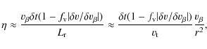
medium must be non-void. A first comparison to the observed Phosphorus
V doublet in the O6 supergiant ![]() Cep
confirms that line profiles calculated from a stochastic 2D model
reproduce observations with a mass-loss rate approximately ten times
higher than that derived from the same lines but assuming optically
thin clumping. Tentatively this may resolve discrepancies between
theoretical predictions, evolutionary constraints, and recent derived
mass-loss rates, and suggests a re-investigation of the clump structure
predicted by current radiation-hydrodynamic models.
Cep
confirms that line profiles calculated from a stochastic 2D model
reproduce observations with a mass-loss rate approximately ten times
higher than that derived from the same lines but assuming optically
thin clumping. Tentatively this may resolve discrepancies between
theoretical predictions, evolutionary constraints, and recent derived
mass-loss rates, and suggests a re-investigation of the clump structure
predicted by current radiation-hydrodynamic models.
Key words: stars: early-type - stars: mass-loss - radiative transfer - line: formation - hydrodynamics - instabilities
1 Introduction
Mass loss through supersonic stellar winds is pivotal for the physical understanding of hot, massive stars and their surroundings. A change of only a factor of two in the mass-loss rate has a dramatic effect on massive star evolution (Meynet et al. 1994). Winds from these stars are described by the line-driven wind theory (Pauldrach et al. 1986; Castor et al. 1975), which traditionally assumes the wind to be stationary, spherically symmetric, and homogeneous. Despite this theory's apparent success (e.g., Vink et al. 2000), evidence for an inhomogeneous and time-dependent wind has over the past years accumulated, recently summarized in the proceedings from the workshop ``Clumping in hot star winds'' (Hamann et al. 2008) and in a general review of mass loss from hot, massive stars (Puls et al. 2008b).
That line-driven winds should be intrinsically unstable was already pointed out by Lucy & Solomon (1970), and was later confirmed first by linear stability analyses and then by direct, radiation-hydrodynamic modeling of the time-dependent wind (e.g., Feldmeier 1995; Owocki et al. 1988; Dessart & Owocki 2005; Owocki & Rybicki 1984), where the line-driven (or line-deshadowing) instability causes a small-scale, inhomogeneous wind in both density and velocity.
Direct observational evidence of a small-scale, clumped stellar
wind has, for O-stars, so far only been given for two objects, ![]() Pup
and HD 93129A (Eversberg et al. 1998; Lépine & Moffat 2008). Much indirect
evidence, however, has arisen from quantitative spectroscopy, where the
standard way of deriving mass-loss rates from observations nowadays is via
line-blanketed, non-LTE (LTE: local thermodynamic equilibrium) model
atmospheres that include a treatment of both the photosphere and the wind.
Wind clumping has been included in such codes (e.g., CMFGEN
Hillier & Miller 1998, PoWR Gräfener et al. 2002, FASTWIND Puls et al. 2005) by
assuming statistically distributed optically thin density clumps
and a void inter-clump medium, while keeping the smooth velocity law. The
major result from this methodology is that any mass-loss rate derived from
smooth models and density-squared diagnostics (
Pup
and HD 93129A (Eversberg et al. 1998; Lépine & Moffat 2008). Much indirect
evidence, however, has arisen from quantitative spectroscopy, where the
standard way of deriving mass-loss rates from observations nowadays is via
line-blanketed, non-LTE (LTE: local thermodynamic equilibrium) model
atmospheres that include a treatment of both the photosphere and the wind.
Wind clumping has been included in such codes (e.g., CMFGEN
Hillier & Miller 1998, PoWR Gräfener et al. 2002, FASTWIND Puls et al. 2005) by
assuming statistically distributed optically thin density clumps
and a void inter-clump medium, while keeping the smooth velocity law. The
major result from this methodology is that any mass-loss rate derived from
smooth models and density-squared diagnostics (
![]() ,
infra-red
and radio emission) needs to be scaled down by the square root of the
clumping factor (which describes the over density of the clumps as compared
to the mean density, see Sect. 2.2). For example,
Crowther et al. (2002), Bouret et al. (2003), and Bouret et al. (2005) have concluded
that a reduction of `smooth' mass-loss rates by factors
,
infra-red
and radio emission) needs to be scaled down by the square root of the
clumping factor (which describes the over density of the clumps as compared
to the mean density, see Sect. 2.2). For example,
Crowther et al. (2002), Bouret et al. (2003), and Bouret et al. (2005) have concluded
that a reduction of `smooth' mass-loss rates by factors ![]() might be
necessary. Furthermore, from a combined optical/IR/radio analysis of a
sample of Galactic O-giants/supergiants, Puls et al. (2006) derived upper limits
on observed rates that were factors of
might be
necessary. Furthermore, from a combined optical/IR/radio analysis of a
sample of Galactic O-giants/supergiants, Puls et al. (2006) derived upper limits
on observed rates that were factors of ![]() lower than previous
lower than previous
![]() estimates based on a smooth wind.
estimates based on a smooth wind.
On the other hand, the strength of UV resonance lines (``P Cygni lines'') in
hot star winds depends linearly on the density and is therefore not believed
to be directly affected by optically thin clumping. By using the Sobolev
with exact integration technique (SEI; cf. Lamers et al. 1987) on
the unsaturated Phosphorus V (PV) lines, Fullerton et al. (2006) for a large
number of Galactic O-stars derived rates that were factors of
![]() lower than corresponding smooth
lower than corresponding smooth
![]() /radio values (provided PV
is the dominant ion in spectral classes O4 to O7). Such large revisions
would conflict with the radiative line-driven wind theory and have dramatic
consequences for the evolution of, and the feedback from, massive stars
(cf. Hirschi 2008; Smith & Owocki 2006). Indeed, a puzzling picture has emerged,
and it appears necessary to ask whether the present treatment of wind
clumping is sufficient. Particularly the assumptions of optically thin
clumps, a void inter-clump medium, and a smooth velocity field may not be
adequate to infer proper rates under certain conditions.
/radio values (provided PV
is the dominant ion in spectral classes O4 to O7). Such large revisions
would conflict with the radiative line-driven wind theory and have dramatic
consequences for the evolution of, and the feedback from, massive stars
(cf. Hirschi 2008; Smith & Owocki 2006). Indeed, a puzzling picture has emerged,
and it appears necessary to ask whether the present treatment of wind
clumping is sufficient. Particularly the assumptions of optically thin
clumps, a void inter-clump medium, and a smooth velocity field may not be
adequate to infer proper rates under certain conditions.
Optically thin vs. optically thick clumps.
Oskinova et al. (2007) used a porosity formalism (Owocki et al. 2004; Feldmeier et al. 2003) to scale the opacity from smooth models and investigate impacts from optically thick clumps on the line profiles ofIn this first paper we attempt to clarify the most important concepts
by conducting a detailed investigation on the synthesis of UV
resonance lines from inhomogeneous two-dimensional (2D) winds. We
create both pseudo-2D, radiation-hydrodynamic wind models and 2D,
stochastic wind models, and produce synthetic line profiles via
Monte-Carlo radiative transfer calculations. We account for and
analyze the effects from a wind clumped in both density and
velocity as well as the effects from a non-void inter-clump
medium. Especially we focus on lines with intermediate line strengths,
comparing the behavior of these lines with the behavior of both
optically thin lines and saturated lines. Follow-up studies will
include a treatment of emission lines (e.g.,
![]() )
and an
extension to 3D, and the development of simplified approaches to
incorporate effects into non-LTE models.
)
and an
extension to 3D, and the development of simplified approaches to
incorporate effects into non-LTE models.
In Sect. 2 we describe the wind models and in Sect. 3 the Monte-Carlo radiative transfer code. First results from 2D inhomogeneous winds are presented in Sect. 4, and an extensive parameter study is carried out in Sect. 5. We discuss some aspects of the interpretations of these results and perform a first comparison to observations in Sect. 6, and summarize our findings and outline future work in Sect. 7.
2 Wind models
![\begin{figure}
\par\includegraphics[angle=90,width=8.8cm,clip]{12842f1a.ps}\includegraphics[width=8.8cm,clip]{12842f1b.eps}
\end{figure}](/articles/aa/full_html/2010/02/aa12842-09/img43.png)
|
Figure 1: Left panel: density contour plots of one stochastic (upper plot) and one RH (FPP, lower plot) model. The Cartesian coordinate Z is on the abscissa and X is on the ordinate. Right panel: density and velocity structures of one slice in one stochastic ( upper) and one RH (FPP, lower) model. Over densities are marked with filled dots. For model parameters and details, see Sect. 2.2. |
| Open with DEXTER | |
For wind models, we use customary spherical coordinates
![]() with r the radial coordinate,
with r the radial coordinate, ![]() the polar angle, and
the polar angle, and ![]() the
azimuthal angle. We assume spherical symmetry in 1D models and symmetry in
the
azimuthal angle. We assume spherical symmetry in 1D models and symmetry in ![]() in 2D models. In all 2D models
in 2D models. In all 2D models ![]() is sliced into
is sliced into
![]() equally sized slices, giving a lateral scale of coherence (or an opening
angle)
equally sized slices, giving a lateral scale of coherence (or an opening
angle)
![]() degrees. This 2D approximation is discussed in
Sect. 6.4. Below we describe the model types primarily used in the
present analysis; two are of stochastic nature and two are of
radiation-hydrodynamic nature.
degrees. This 2D approximation is discussed in
Sect. 6.4. Below we describe the model types primarily used in the
present analysis; two are of stochastic nature and two are of
radiation-hydrodynamic nature.
2.1 Radiation-hydrodynamic wind models
We use the time-dependent, radiation-hydrodynamic (hereafter RH) wind models from Puls et al. (1993, hereafter ``POF''), calculated by Owocki, and from Feldmeier et al. (1997, hereafter ``FPP''), and the reader is referred to these papers for details. Here we summarize a few important aspects. POF assume a 1D, spherically symmetric outflow, and circumvent a detailed treatment of the wind energy equation by assuming an isothermal flow. Perturbations are triggered by photospheric sound waves. The wind consists of 800 radial points, extending to roughly 5 stellar radii. FPP also assume a 1D, spherically symmetric outflow, but include a treatment of the energy equation. Perturbations are triggered either by photospheric sound waves or by Langevin perturbations that mimic photospheric turbulence. The wind consists of 4000 radial points, extending to roughly 30 stellar radii. Tests have shown that the FPP winds yield similar results for both flavors of perturbations, and, for simplicity, we therefore use only the results of the turbulence model.Due to the computational cost of obtaining the line force, only initial
attempts to 2D RH simulations have been carried out
(Dessart & Owocki 2003,2005). These authors first used a strictly radial
line force, yielding a complete lateral incoherent structure due to
Rayleigh-Taylor or thin-shell instabilities, and in the follow-up study uses
a restricted 3-ray approach to approximate the lateral line drag, yielding a
larger lateral coherence but lacking quantitative results. Therefore, and
because of the general dominance of the radial component in the radiative
driving, we create fragmented 2D wind models from our 1D RH ones by
assembling snapshots in the ![]() direction, assuming independence
between each slice consisting of a pure radial flow. After the polar angle
has been sliced into
direction, assuming independence
between each slice consisting of a pure radial flow. After the polar angle
has been sliced into
![]() equally sized slices, one random snapshot
is selected to represent each slice. This method for creating more-D models
from 1D ones is essentially the same as the ``patch method'' used by
Dessart & Owocki (2002), when synthesizing emission lines for Wolf-Rayet stars,
and the method used by, e.g., Oskinova et al. (2004), when synthesizing X-ray
line emission from stochastic wind models. Figure 1 displays
typical velocity and density structures from this type of 2D model.
equally sized slices, one random snapshot
is selected to represent each slice. This method for creating more-D models
from 1D ones is essentially the same as the ``patch method'' used by
Dessart & Owocki (2002), when synthesizing emission lines for Wolf-Rayet stars,
and the method used by, e.g., Oskinova et al. (2004), when synthesizing X-ray
line emission from stochastic wind models. Figure 1 displays
typical velocity and density structures from this type of 2D model.
2.2 Stochastic wind models
We also study clumpy wind structures created by means of distorting a
smooth, stationary, and spherically symmetric wind via stochastic
procedures. This allows us to investigate the impacts from, and to set
constraints on, different key parameters without being limited by the
values predicted by the RH simulations. For the underlying smooth
winds we adopt a standard ![]() velocity law
velocity law
![]() .
Here and throughout the paper, we
measure all velocities in units of the terminal velocity,
.
Here and throughout the paper, we
measure all velocities in units of the terminal velocity,
![]() ,
and all distances and length scales in units of the
stellar radius,
,
and all distances and length scales in units of the
stellar radius, ![]() .
b is given by
.
b is given by
![]() ,
the
velocity at the base of the wind.
,
the
velocity at the base of the wind.
![]() is assumed,
roughly corresponding to the sound speed. For a given
is assumed,
roughly corresponding to the sound speed. For a given ![]() ,
the
homogeneous density structure then follows directly from the equation
of continuity. We choose
,
the
homogeneous density structure then follows directly from the equation
of continuity. We choose ![]() ,
which is appropriate for a
standard O-star wind and allows us to derive simple analytic
expressions for wind masses and flight times.
,
which is appropriate for a
standard O-star wind and allows us to derive simple analytic
expressions for wind masses and flight times.
A model clumped in density.
First we consider a two component density structure consisting of clumps and a rarefied inter-clump medium (hereafter ICM), but keep theThe average distance between clumps thus is
![]() ,
i.e. clumps are spatially closer in the inner wind than in the outer
wind, and for example
,
i.e. clumps are spatially closer in the inner wind than in the outer
wind, and for example
![]() (in
(in
![]() )
gives an
average clump separation of 0.5 (in
)
gives an
average clump separation of 0.5 (in ![]() )
at the point where v
= 1 (in
)
at the point where v
= 1 (in
![]() ). We further assume that the clumps preserve mass
and lateral angle when propagating outwards, and that the underlying
model's total wind mass is conserved within every slice. This radial
clump distribution is the same as the one used by
Oskinova et al. (2006) when simulating X-ray emission from O-stars, but
differs from the one used by Oskinova et al. (2007) when investigating
porosity effects on resonance lines (see discussion in
Sect. 6.5). The radial clump widths are here
calculated from the actual wind geometry and clump distribution by
assuming a volume filling factor
). We further assume that the clumps preserve mass
and lateral angle when propagating outwards, and that the underlying
model's total wind mass is conserved within every slice. This radial
clump distribution is the same as the one used by
Oskinova et al. (2006) when simulating X-ray emission from O-stars, but
differs from the one used by Oskinova et al. (2007) when investigating
porosity effects on resonance lines (see discussion in
Sect. 6.5). The radial clump widths are here
calculated from the actual wind geometry and clump distribution by
assuming a volume filling factor ![]() ,
defined as the
fractional volume of the dense gas
,
defined as the
fractional volume of the dense gas![]() . A
related quantity is the clumping factor
. A
related quantity is the clumping factor

as defined by Owocki et al. (1988), where angle brackets denote temporal averages. Identifying temporal with spatial averages one may write for a two component medium (cf. Abbott et al. 1981)
![\begin{displaymath}f_{\rm cl} = \frac{f_{\rm v}+(1-f_{\rm v})x_{\rm ic}^2}{[f_{\rm v}+(1-f_{\rm v})x_{\rm ic}]^2},
\end{displaymath}](/articles/aa/full_html/2010/02/aa12842-09/img62.png)
with

the ratio of low- to high-density gas (subscript ic denotes inter-clump and cl denotes clump). For a void (
A model clumped in density and velocity.
Next we consider also a non-monotonic velocity law, using the spatial distribution and widths of the clumps described in the previous paragraph. The RH simulations indicate that, generally, strong shocks separate denser and slower material from rarefied regions with higher velocities. Building on this basic result, we now modify the velocity fields in our stochastic models by adding a random perturbation to the local
where
Overall, the above treatment provides a phenomenological description of the non-monotonic velocity field seen in RH simulations. The description differs from the one suggested by Owocki (2008), who uses only one parameter to characterize the velocity field (whereas we have two). Our new formulation is motivated by both observational and modeling constraints from strong and intermediate lines, as discussed in Sect. 6.5.
The basic parameters defining a stochastic model are listed in
Table 1. Figure 1 (right panel) shows the
density and velocity structures of one slice in a stochastic model,
with density parameters
![]() ,
,
![]() ,
,
![]() ,
and velocity parameters
,
and velocity parameters
![]() and
and
![]() .
Clump positions have been highlighted
with filled dots and a comparison to a RH model (FPP) is given. In the
RH model, we have identified clump positions by highlighting all
density points with values higher than the corresponding smooth
model. The left panel shows the density contours of the same models,
where, for clarity, only the wind to r=5 is displayed.
.
Clump positions have been highlighted
with filled dots and a comparison to a RH model (FPP) is given. In the
RH model, we have identified clump positions by highlighting all
density points with values higher than the corresponding smooth
model. The left panel shows the density contours of the same models,
where, for clarity, only the wind to r=5 is displayed.
Table 1: Basic parameters defining a stochastic wind model clumped in density and with a non-monotonic velocity field.
| Figure 2: Non-monotonic velocity field and corresponding parameters in a stochastic model. |
|
| Open with DEXTER | |
3 Radiative transfer
To compute synthetic line profiles from the wind models, we have developed a Monte-Carlo radiative transfer code (MC-2D) that treats resonance line formation in a spherical and axially symmetric wind using an ``exact'' formulation (e.g., without resorting to the Sobolev approximation). The restriction to 2D is of course a shortage, but has certain geometrical and computational advantages and should be sufficient for the study of general properties, as discussed in Sect. 6.4. A thorough description and verification of the code can be found in Appendix A.Photons are released from the lower boundary (the photosphere) and each path is followed until the photon has either left the wind or been backscattered into the photosphere. Basic assumptions are a line-free continuum with no limb darkening emitted at the lower boundary, no continuum absorption in the wind, pure scattering lines, instantaneous re-emission, and no overlapping lines (i.e., singlets). These simplifying assumptions, except for doublet formation, are all believed to be of minor importance to the basic problem. By the restriction to singlet line formation we avoid confusion between effects on the line profiles caused by line overlaps and by other important parameters, but on the other hand it also prevents a direct comparison to observations for many cases (but see Sect. 6.6). A consistent treatment of doublet formation will be included in the follow-up study.
4 First results from 2D inhomogeneous winds
Throughout this section we assume a thermal velocity,
![]() (in units of
(in units of
![]() and
and ![]()
![]() ,
appropriate for a
standard O-star wind), and apply no microturbulence. After a brief
discussion on the impact of the observer's position and opening angles, we
concentrate on investigating the
formation of strong, intermediate, and weak lines. In our
definition, an intermediate line is characterized by a line
strength
,
appropriate for a
standard O-star wind), and apply no microturbulence. After a brief
discussion on the impact of the observer's position and opening angles, we
concentrate on investigating the
formation of strong, intermediate, and weak lines. In our
definition, an intermediate line is characterized by a line
strength![]()
![]() chosen
such as to almost precisely reach the saturation limit in a smooth
model (cf. Fig. 3).
chosen
such as to almost precisely reach the saturation limit in a smooth
model (cf. Fig. 3).
By investigating these different line types, we account for the tight
constraints that exist for each flavor: i) weak lines should
be independent of density-clumping properties as long as the clumps
remain optically thin; ii) for intermediate lines either
smooth models overestimate the profile strengths or mass-loss rates
are lower than previously thought (e.g. the PV problem, see
Sect. 1), and iii) strong saturated lines
are clearly present in hot star UV spectra, and observed features need
to be reproduced, such as high velocity (>
![]() )
absorption, the
black absorption trough, and the reduction of re-emitted flux blueward
of the line center.
)
absorption, the
black absorption trough, and the reduction of re-emitted flux blueward
of the line center.
4.1 Observer's position and opening angles
The observed spectrum as calculated from a 2D wind structure depends on the observer's placement relative to the star (see Appendix A). As it turns out, however, this dependence is relatively weak in both the stochastic and the RH models (the latter is demonstrated in the upper panel of Fig. 3). Tests have shown that the variability of the line profile's emission part is insignificant. The variability of the absorption part may be detectable, at least near the blue edge, but is still insignificant for the integrated profile strength; the equivalent width of the absorption part is almost independent of the observer's position. Also the opening angle,Because our main interest here is the general behavior of the line
profiles, we choose to work only with
![]() and profiles
averaged over all observer angles from here on. Working with averaged
line profiles has great computational advantages, because roughly a
factor of
and profiles
averaged over all observer angles from here on. Working with averaged
line profiles has great computational advantages, because roughly a
factor of
![]() fewer photons are needed.
fewer photons are needed.
![\begin{figure}
\par\includegraphics[width=8.8cm,clip]{12842f3a.eps}\par\includegraphics[width=8.8cm,clip]{12842f3b.eps}
\end{figure}](/articles/aa/full_html/2010/02/aa12842-09/img95.png)
|
Figure 3:
Synthetic line profiles calculated from 2D RH models. The
abscissa is the dimensionless frequency x (Eq. (A.5)),
normalized to the terminal velocity, and the ordinate is the flux
normalized to the continuum. Upper panel: profiles from
POF models with
|
| Open with DEXTER | |
4.2 Radiation-hydrodynamic models
Figure 3 (lower panel) shows line profiles from FPP and
POF hydrodynamical models. For the strong lines, the constraints
stated in the beginning of this section are reproduced without
adopting a highly supersonic and artificial microturbulence. These
features arise because of the multiple resonance zones in a
non-monotonic velocity field, and are present in spherically symmetric
RH profiles as well (see POF for a comprehensive discussion); the main
difference between 1D and 2D is a smoothing effect, partly stemming
from averaging over all observer angles (see above). The absorption
at velocities higher than the terminal is stronger in FPP than in POF,
due to both a higher velocity dispersion and a larger extent of the
wind (
![]() as compared to
as compared to
![]() ,
see
Sect. 2.1); more overdense regions are encountered in the
outermost wind, which (because of the flatness of the velocity field)
leads to an increased probability to absorb at almost the same
velocities.
,
see
Sect. 2.1); more overdense regions are encountered in the
outermost wind, which (because of the flatness of the velocity field)
leads to an increased probability to absorb at almost the same
velocities.
For the intermediate lines, we again see the qualitative features of
the strong lines, though less prominent. As compared to smooth models,
a minor absorption reduction is present at velocities lower
than the terminal, but compensated by the blue edge
smoothing. Therefore the equivalent width of the line profile's
absorption part in the FPP model is approximately equal to that of the
smooth model, whereas in the POF model it is reduced by ![]()
![]() .
This minor reduction agrees with that found by Owocki (2008),
and is not strong enough to explain the observations without having to
invoke a very low mass-loss rate.
.
This minor reduction agrees with that found by Owocki (2008),
and is not strong enough to explain the observations without having to
invoke a very low mass-loss rate.
For the weak lines, the absorption part is marginally stronger than from a smooth, 1D model.
4.3 Stochastic models
Table 2: Primary stochastic wind models and parameters.
![\begin{figure}
\par {\includegraphics[width=10.9cm,clip]{12842f4.eps} }
\end{figure}](/articles/aa/full_html/2010/02/aa12842-09/img102.png)
|
Figure 4:
Left panels: solid lines display total line profiles
and the absorption part for the default stochastic model (see
Table 2), with
|
| Open with DEXTER | |
In this subsection we use a ``default'' 2D, stochastic model with parameters as specified in Table 2. By comparing this model to models in which one or more parameters are changed, we demonstrate key effects in the behavior of the line profiles.
Strong lines.
For strong lines, the line profiles from the default model reproduce the observational constraints described in the first paragraph of this section. As in the RH models, we apply no microturbulence. Figure 4 (left panels) demonstrates the importance of the ICM in the default model; the absorption part of a very strong line is not saturated whenIntermediate lines.
For intermediate lines, the line profiles from the default model display the main observational requirement if to avoid a drastic reduction in ``smooth'' mass-loss ratesWe have identified
![]() as a critical parameter for the formation
of intermediate lines. The importance of the velocity spans of the clumps
is well illustrated by the absorption part profiles in Fig. 4
(lower-left panel, middle plot). The absorption is much stronger in the
comparison model with
as a critical parameter for the formation
of intermediate lines. The importance of the velocity spans of the clumps
is well illustrated by the absorption part profiles in Fig. 4
(lower-left panel, middle plot). The absorption is much stronger in the
comparison model with
![]() than in the default
model with
than in the default
model with
![]() ,
because the former model covers
more of the total velocity space within the clumps, thereby closing
the gaps between the clumps. Consequently the wind may, on average,
absorb at many more wavelengths.
,
because the former model covers
more of the total velocity space within the clumps, thereby closing
the gaps between the clumps. Consequently the wind may, on average,
absorb at many more wavelengths.
In principle, however, this effect is counteracted by a decrease in the
clump's optical depths, because of the now higher velocity gradients
(
![]() ). Consider the radial Sobolev
optical depth (proportional to
). Consider the radial Sobolev
optical depth (proportional to
![]() ,
see
Appendix A) in a stochastic wind model. As compared to a smooth
model, the density inside a clump is enhanced by a factor of
,
see
Appendix A) in a stochastic wind model. As compared to a smooth
model, the density inside a clump is enhanced by a factor of
![]() (assuming a negligible ICM), but also the velocity gradient is
enhanced by a factor of
(assuming a negligible ICM), but also the velocity gradient is
enhanced by a factor of
![]() .
Thus we may write for
the radial Sobolev optical depth inside a clump,
.
Thus we may write for
the radial Sobolev optical depth inside a clump,

where ``sm'' indicates a quantity from a smooth wind, and the expression to the right is valid for an underlying
Finally, the prominent absorption dip toward the blue edge in the default model turns out to be a quite general feature of our stochastic models, and is discussed in Sects. 5.1 and 6.2.
Weak lines.
The statistical treatment of density clumping included in atmospheric codes such as CMFGEN, PoWR, and FASTWIND is valid for optically thin clumps and a negligible ICM, and gives no direct effect on resonance lines scaling linearly with density. Here we test this prediction using detailed radiative transfer![\begin{figure}
\par\includegraphics[width=8.8cm,clip]{12842f5.eps}
\end{figure}](/articles/aa/full_html/2010/02/aa12842-09/img120.png)
|
Figure 5: Velocity ( upper panel) and density ( lower panel) structures for one slice in POF (dashed) and RHcopy (dotted), see Table 2. Solid lines are the corresponding smooth structures, and clumps are highlighted as in Fig. 1. |
| Open with DEXTER | |
4.4 Comparison between stochastic and radiation-hydrodynamic models
Our stochastic wind models have been constructed to contain all
essential ingredients of the RH models. Therefore they should also
reproduce the RH results, at least qualitatively, if a suitable parameter
set is chosen. To test this we used the POF model. In this model, the
clumping factor increases drastically at
![]() ,
from
,
from
![]() to
to
![]() ,
after which it stays
basically constant. The average clump separation in the outer wind is
roughly half a stellar radius. Important for the velocity field is
that the velocity spans of the clumps are generally larger
than corresponding ``
,
after which it stays
basically constant. The average clump separation in the outer wind is
roughly half a stellar radius. Important for the velocity field is
that the velocity spans of the clumps are generally larger
than corresponding ``![]() spans'', i.e.,
spans'', i.e.,
![]() (this is the case in FPP as well), a characteristic behavior that
primarily affects the intermediate lines (details will be discussed in
Sect. 6.3). Finally, a suitable
(this is the case in FPP as well), a characteristic behavior that
primarily affects the intermediate lines (details will be discussed in
Sect. 6.3). Finally, a suitable ![]() can be assigned
from the position of the blue edge in a strong line calculated from
POF. Table 2 (entry RHcopy) summarizes all parameters used
to create this stochastic, ``pseudo-RH'' model. Figure 5
displays one slice of the velocity and density structures in the POF
and RHcopy models, and Fig. 4 (right panels) displays
the line profiles.
can be assigned
from the position of the blue edge in a strong line calculated from
POF. Table 2 (entry RHcopy) summarizes all parameters used
to create this stochastic, ``pseudo-RH'' model. Figure 5
displays one slice of the velocity and density structures in the POF
and RHcopy models, and Fig. 4 (right panels) displays
the line profiles.
The line profiles of POF are matched reasonably well by RHcopy. The
intermediate lines again demonstrate the importance of the velocity spans of
the clumps; for an alternative model with
![]() ,
there is much less absorption in the stochastic model than in POF, i.e., we
encounter the same effect as discussed in the previous subsection. We
conclude that in RH models it is the large velocity spans inside the density
enhancements that prevent a reduction in profile strength (as compared to
smooth models) for intermediate lines.
,
there is much less absorption in the stochastic model than in POF, i.e., we
encounter the same effect as discussed in the previous subsection. We
conclude that in RH models it is the large velocity spans inside the density
enhancements that prevent a reduction in profile strength (as compared to
smooth models) for intermediate lines.
5 Parameter study
Having established basic properties, we now use our stochastic models to analyze the influence from different key parameters in more detail. First, however, we introduce a quantity that turns out to be particularly useful for our later discussion.
5.1 The effective escape ratio
![\begin{figure}
\par\includegraphics[width=8.8cm,clip]{12842f6.eps}
\end{figure}](/articles/aa/full_html/2010/02/aa12842-09/img124.png)
|
Figure 6:
Left: schematic of |
| Open with DEXTER | |
For the important intermediate lines, it is reasonable to assume that
the clumps are optically thick and the ICM negligible (see
Sect. 4.3 and the next paragraph). Under these assumptions, a
decisive quantity for photon absorption will be the velocity gap not covered by the clumps, as compared to the thermal velocity (the
latter determining the width of the resonance zone in which the photon
may interact with the wind material). This is illustrated in the left
panel of Fig. 6, and we shall call this quantity the
``effective escape ratio''

where
For the wind geometry used in our stochastic models, we may write (see
Appendix B for a derivation)
where
Using the parameters of our default model, Fig. 6 (right panel)
displays ![]() as a function of velocity and shows that
as a function of velocity and shows that ![]() increases
rapidly in the inner wind, reaches a maximum at
increases
rapidly in the inner wind, reaches a maximum at
![]() ,
and then
drops in the outer wind. To compare this behavior with that of the line
profiles, we can associate absorption at some frequency
,
and then
drops in the outer wind. To compare this behavior with that of the line
profiles, we can associate absorption at some frequency
![]() with
the corresponding value of the velocity, because absorption occurs at
with
the corresponding value of the velocity, because absorption occurs at
![]() (radial photons dominate). In the
default model's absorption-part line profile (see Fig. 4,
the middle plot in the lower-left panel), a strong de-saturation occurs
directly after the clumping is set to start (at r=1.3,
(radial photons dominate). In the
default model's absorption-part line profile (see Fig. 4,
the middle plot in the lower-left panel), a strong de-saturation occurs
directly after the clumping is set to start (at r=1.3,
![]() ),
followed by a maximum at
),
followed by a maximum at
![]() ,
and finally an
absorption dip toward the blue edge. The behavior of the line profile is
thus well mapped by
,
and finally an
absorption dip toward the blue edge. The behavior of the line profile is
thus well mapped by ![]() ,
and we may explain the absorption dip as a
consequence of the low value of
,
and we may explain the absorption dip as a
consequence of the low value of ![]() in the outer wind, which in turn
stems from the slow variation of the velocity field (i.e., from radially
extended resonance zones).
in the outer wind, which in turn
stems from the slow variation of the velocity field (i.e., from radially
extended resonance zones).
5.2 Density parameters
To isolate density-clumping effects, we use a smooth ![]() velocity law in this subsection. Despite the smooth velocity field,
there are still holes in velocity space (because of the density
clumping, at the locations where the ICM is present), and the
expression for
velocity law in this subsection. Despite the smooth velocity field,
there are still holes in velocity space (because of the density
clumping, at the locations where the ICM is present), and the
expression for ![]() (Eq. (7)) remains valid. Since a
smooth velocity field corresponds to
(Eq. (7)) remains valid. Since a
smooth velocity field corresponds to
![]() ,
also
the run of
,
also
the run of ![]() is equal to the one displayed in
Fig. 6. In this subsection we work only with integrated
profile strengths (characterized by the equivalent width
is equal to the one displayed in
Fig. 6. In this subsection we work only with integrated
profile strengths (characterized by the equivalent width
![]() of the line's absorption part). The shapes of the line profiles are
discussed in Sect. 6.1.
of the line's absorption part). The shapes of the line profiles are
discussed in Sect. 6.1.
Figure 7 shows
![]() as a function of
as a function of ![]() ,
for smooth models as well as for stochastic models with and without a
contributing ICM. The figure directly tells: i) The default model
(
,
for smooth models as well as for stochastic models with and without a
contributing ICM. The figure directly tells: i) The default model
(
![]() )
for the intermediate line (
)
for the intermediate line (
![]() )
displays
a
)
displays
a
![]() corresponding to a smooth model with a
corresponding to a smooth model with a ![]() roughly ten times lower. ii) Lines never saturate if the ICM is
(almost) void. iii) The run of
roughly ten times lower. ii) Lines never saturate if the ICM is
(almost) void. iii) The run of
![]() for the smooth and
clumped models decouple well before
for the smooth and
clumped models decouple well before ![]() reaches unity. iv) For
intermediate lines, the response of
reaches unity. iv) For
intermediate lines, the response of
![]() on variations of
on variations of
![]() is weak for clumped models. Points one to three confirm
our findings from Sect. 4.3.
is weak for clumped models. Points one to three confirm
our findings from Sect. 4.3.
A variation of ![]() in the stochastic models affects
primarily the high
in the stochastic models affects
primarily the high ![]() part (
part (
![]() )
of the curves in
Fig. 7. For example, lowering
)
of the curves in
Fig. 7. For example, lowering ![]() in the model with a void ICM results in an upward shift
of the dashed curve and vice versa. To obtain saturation with a void ICM,
in the model with a void ICM results in an upward shift
of the dashed curve and vice versa. To obtain saturation with a void ICM,
![]() is required, which may be understood in terms of
Eq. (7).
For
is required, which may be understood in terms of
Eq. (7).
For
![]() ,
the
,
the ![]() -values corresponding to the default model
are decreased by a factor of ten, and
-values corresponding to the default model
are decreased by a factor of ten, and ![]() reaches a maximum of only about
unity, with even lower values for the majority of the velocity space (cf.
Fig. 6, right panel). The velocity gaps between the clumps then
become closed, and the line saturates. In this situation, however, the
intermediate line becomes saturated as well, again demonstrating the
necessity of a non-void ICM to simultaneously saturate a strong line
and not saturate an intermediate line. Only a properly chosen
reaches a maximum of only about
unity, with even lower values for the majority of the velocity space (cf.
Fig. 6, right panel). The velocity gaps between the clumps then
become closed, and the line saturates. In this situation, however, the
intermediate line becomes saturated as well, again demonstrating the
necessity of a non-void ICM to simultaneously saturate a strong line
and not saturate an intermediate line. Only a properly chosen
![]() parameter ensures that the velocity gaps between the clumps become filled by
low-density material able to absorb at strong line opacities, but
not (or only marginally) at opacities corresponding to intermediate
lines.
parameter ensures that the velocity gaps between the clumps become filled by
low-density material able to absorb at strong line opacities, but
not (or only marginally) at opacities corresponding to intermediate
lines.
When varying
![]() ,
the primary change occurs at the high
,
the primary change occurs at the high ![]() end of Fig. 7. For higher (lower) values of
end of Fig. 7. For higher (lower) values of
![]() ,
this
part becomes shifted to the left (right), and the curve decouples
earlier (later) from the corresponding curve for the void ICM. A
higher ICM density obviously means that the ICM starts absorbing
photons at lower line strengths and vice versa. Thus, observed
saturated lines could potentially be used to derive the ICM density
(or at least to infer a lower limit), if the mass-loss rate
(and abundance) is known from other diagnostics.
,
this
part becomes shifted to the left (right), and the curve decouples
earlier (later) from the corresponding curve for the void ICM. A
higher ICM density obviously means that the ICM starts absorbing
photons at lower line strengths and vice versa. Thus, observed
saturated lines could potentially be used to derive the ICM density
(or at least to infer a lower limit), if the mass-loss rate
(and abundance) is known from other diagnostics.
The behavior of the absorption with respect to the volume filling
factor is as expected from the expression for ![]() ;
the higher
;
the higher ![]() ,
the lower the value of
,
the lower the value of ![]() ,
and the stronger the
absorption. This is because a higher
,
and the stronger the
absorption. This is because a higher ![]() for a fixed
for a fixed ![]() implies that the clumps become more extended, whereas the distances
between clump centers remain unaffected. Consequently, a larger
fraction of the total wind velocity is covered by the clumps, leading
to stronger absorption. For weak lines (
implies that the clumps become more extended, whereas the distances
between clump centers remain unaffected. Consequently, a larger
fraction of the total wind velocity is covered by the clumps, leading
to stronger absorption. For weak lines (
![]() ), the
ratio
), the
ratio
![]() deviates significantly from
unity only when
deviates significantly from
unity only when
![]() .
Only for such low values can high
enough clump densities be produced so that the clumps start to become
optically thick.
.
Only for such low values can high
enough clump densities be produced so that the clumps start to become
optically thick.
![\begin{figure}
\par\includegraphics[width=8.8cm,clip]{12842f7.eps}
\end{figure}](/articles/aa/full_html/2010/02/aa12842-09/img145.png)
|
Figure 7:
Equivalent widths
|
| Open with DEXTER | |
From Fig. 7 it is obvious that, generally, clumped
models have a different (slower) response in
![]() to an
increase in
to an
increase in ![]() than do smooth models. This behavior may be
observationally tested using UV resonance doublets (Massa et al. 2008),
because the only parameter that differs between the two line
components is the oscillator strength. Thus, if a smooth wind model is
used and the fitted ratio of line strengths (i.e.,
than do smooth models. This behavior may be
observationally tested using UV resonance doublets (Massa et al. 2008),
because the only parameter that differs between the two line
components is the oscillator strength. Thus, if a smooth wind model is
used and the fitted ratio of line strengths (i.e.,
![]() )
does not correspond to the expected
ratio of oscillator strengths, one may interpret this as a signature
of a clumped wind. Such behavior was found by Massa et al. (2008), where
the observed ratios of the blue to red component of Si IV
)
does not correspond to the expected
ratio of oscillator strengths, one may interpret this as a signature
of a clumped wind. Such behavior was found by Massa et al. (2008), where
the observed ratios of the blue to red component of Si IV
![]() 1394,1403 in B supergiants showed a wide spread
between unity and the expected factor of two. This result indicates
precisely the slow response to an increase in
1394,1403 in B supergiants showed a wide spread
between unity and the expected factor of two. This result indicates
precisely the slow response to an increase in ![]() that is
consistent with inhomogeneous wind models such as those presented
here, but not with smooth ones. In inhomogeneous models, the expected
profile strength (or
that is
consistent with inhomogeneous wind models such as those presented
here, but not with smooth ones. In inhomogeneous models, the expected
profile strength (or
![]() )
ratio between two doublet
components will depend on the adopted clumping parameters (as
demonstrated by Fig. 7 and the discussion above) and may
in principle take any value in the range found by
Massa et al. That is, while a profile-strength ratio
deviating from the value expected by smooth models might be a clear
indication of a clumped wind, the opposite is not necessarily an
indication of a smooth wind. Furthermore, the degeneracy between a
variation of clumping parameters and
)
ratio between two doublet
components will depend on the adopted clumping parameters (as
demonstrated by Fig. 7 and the discussion above) and may
in principle take any value in the range found by
Massa et al. That is, while a profile-strength ratio
deviating from the value expected by smooth models might be a clear
indication of a clumped wind, the opposite is not necessarily an
indication of a smooth wind. Furthermore, the degeneracy between a
variation of clumping parameters and ![]() suggests that
un-saturated resonance lines should be used primarily as consistency
tests for mass-loss rates derived from other diagnostics rather than
as direct mass-loss estimators. We will return to this problem in
Sect. 6.6, where a first comparison to observations is
performed for the PV doublet.
suggests that
un-saturated resonance lines should be used primarily as consistency
tests for mass-loss rates derived from other diagnostics rather than
as direct mass-loss estimators. We will return to this problem in
Sect. 6.6, where a first comparison to observations is
performed for the PV doublet.
5.3 Velocity parameters
The jump velocity parameter,![\begin{figure}
\par\includegraphics[width=8.8cm,clip]{12842f8.eps}
\end{figure}](/articles/aa/full_html/2010/02/aa12842-09/img149.png)
|
Figure 8:
Upper: velocity structures (one slice) in
two stochastic models with density-clumping parameters as for the
default model, and different velocity parameters. Dashed:
|
| Open with DEXTER | |
In Sects. 4.3 and 4.4, we showed that a higher value of the
clumps' velocity spans led to stronger absorption for intermediate
lines. In principle this is as expected from Eq. (7), where ![]() always decreases with increasing
always decreases with increasing
![]() .
However, with the very high value of
.
However, with the very high value of
![]() used in, e.g., the RHcopy model, one realizes that
used in, e.g., the RHcopy model, one realizes that ![]() in
Eq. (7) becomes identically zero, because
in
Eq. (7) becomes identically zero, because
![]() .
An
.
An ![]() corresponds to the whole velocity
space being covered by clumps, and the saturation limit should be
reached. As is clear from Fig. 4, however, this is not
the case. This points out two important details not included when
deriving the expression for
corresponds to the whole velocity
space being covered by clumps, and the saturation limit should be
reached. As is clear from Fig. 4, however, this is not
the case. This points out two important details not included when
deriving the expression for ![]() and interpreting the absorption in
terms of this quantity, namely that clumps are distributed randomly
(with
and interpreting the absorption in
terms of this quantity, namely that clumps are distributed randomly
(with ![]() determining only the average distances between them)
and that the parameter
determining only the average distances between them)
and that the parameter ![]() allows for an asymmetry in the
velocities of the clumps' starting points (see
Sect. 2.2). These two issues lead to overlapping
velocity spans for some of the clumps, whereas for others there is
still a velocity gap left between them, through which the radiation
can escape. Therefore the profiles do not reach complete saturation,
despite that on average
allows for an asymmetry in the
velocities of the clumps' starting points (see
Sect. 2.2). These two issues lead to overlapping
velocity spans for some of the clumps, whereas for others there is
still a velocity gap left between them, through which the radiation
can escape. Therefore the profiles do not reach complete saturation,
despite that on average ![]() .
This illustrates some inherent limitations when trying to interpret
line formation in terms of a simplified quantity such as
.
This illustrates some inherent limitations when trying to interpret
line formation in terms of a simplified quantity such as ![]() .
.
The impact from the velocity spans of the clumps on the line profiles
also depends on the density-clumping parameters. To achieve
approximately the same level of absorption, a higher value of
![]() was required in the RHcopy model (
was required in the RHcopy model (
![]() )
than in the default model (
)
than in the default model (
![]() ), see
Fig. 4. Since
), see
Fig. 4. Since
![]() (see Appendix B), the actual velocity spans of
the clumps are different for different density-clumping parameters,
even if
(see Appendix B), the actual velocity spans of
the clumps are different for different density-clumping parameters,
even if
![]() remains unchanged.
remains unchanged.
By changing the sign of ![]() in the default model (that is, assuming a
positive velocity gradient inside the clumps), we have found that our
results qualitatively depend only on
in the default model (that is, assuming a
positive velocity gradient inside the clumps), we have found that our
results qualitatively depend only on
![]() .
Some details differ though. For example, a
.
Some details differ though. For example, a
![]() in our stochastic
models permits absorption at velocities higher than the terminal one also
within the clumps, whereas
in our stochastic
models permits absorption at velocities higher than the terminal one also
within the clumps, whereas
![]() restricts the clump velocities to
below the local
restricts the clump velocities to
below the local ![]() (see Fig. 2). In this matter
(see Fig. 2). In this matter
![]() plays a role as well, since
plays a role as well, since ![]() controls where, with
respect to the local
controls where, with
respect to the local ![]() ,
the clumps begin. For reasonable values
of
,
the clumps begin. For reasonable values
of ![]() ,
however, its influence is minor on lines where the ICM is
insignificant. Finally, tests have confirmed that optically thin lines are
only marginally affected when varying
,
however, its influence is minor on lines where the ICM is
insignificant. Finally, tests have confirmed that optically thin lines are
only marginally affected when varying
![]() .
.
6 Discussion
6.1 The shapes of the intermediate lines
![\begin{figure}
\par\includegraphics[width=8.8cm,clip]{12842f9.eps}
\end{figure}](/articles/aa/full_html/2010/02/aa12842-09/img154.png)
|
Figure 9:
Total, absorption part, and re-emission part line profiles
for 1D, smooth models with
|
| Open with DEXTER | |
For intermediate lines, the shape of the absorption part of the default
model differs significantly from the shape of a smooth model (see
Fig. 4, the middle plot in the lower-left panel). We showed
in Sect. 5.1 that the shapes could be qualitatively understood by the
behavior of ![]() .
This is further demonstrated here by scaling the line strength parameter of
a 1D, smooth model, using a parameterization
.
This is further demonstrated here by scaling the line strength parameter of
a 1D, smooth model, using a parameterization
![]() outside the radius r=1.3 where clumping is assumed to start.
Figure 9 displays the line profiles of 1D, smooth models with
outside the radius r=1.3 where clumping is assumed to start.
Figure 9 displays the line profiles of 1D, smooth models with
![]() and
and
![]() .
These profiles are compared to
those calculated from a ``real'' 2D stochastic model with density-clumping
parameters as the default model, but with a
.
These profiles are compared to
those calculated from a ``real'' 2D stochastic model with density-clumping
parameters as the default model, but with a ![]() velocity field.
velocity field. ![]() was calculated from Eq. (7), using the parameters of the default
model and a
was calculated from Eq. (7), using the parameters of the default
model and a ![]() velocity law, and the factor of 2 in the denominator
of the scaled
velocity law, and the factor of 2 in the denominator
of the scaled ![]() was chosen so that the integrated profile
strength of the 2D model was roughly reproduced. From Fig. 9
it is clear that the 1D model with scaled
was chosen so that the integrated profile
strength of the 2D model was roughly reproduced. From Fig. 9
it is clear that the 1D model with scaled ![]() well reproduces the 2D results, indicating that indeed
well reproduces the 2D results, indicating that indeed ![]() governs the shape of the line
profile. We notice also that these profiles display a completely black
absorption dip in the outermost wind, as opposed to the default model with a
non-monotonic velocity field (see Fig. 4, the middle plot in
the lower-left panel). This is because the
governs the shape of the line
profile. We notice also that these profiles display a completely black
absorption dip in the outermost wind, as opposed to the default model with a
non-monotonic velocity field (see Fig. 4, the middle plot in
the lower-left panel). This is because the ![]() velocity field does not
allow for any clumps to overlap in velocity space (see the discussion in
Sect. 5.3), making the mapping of
velocity field does not
allow for any clumps to overlap in velocity space (see the discussion in
Sect. 5.3), making the mapping of ![]() almost perfect.
almost perfect.
Let us also point out that the line shapes can be somewhat altered
by using a different velocity law, e.g.,
![]() .
Such a change would
affect the distances between clumps as well as the Sobolev length, and
thereby the line shapes of both absorption and re-emission profiles.
However, in all cases is the shape of the re-emission part similar in the
clumped and smooth models.
.
Such a change would
affect the distances between clumps as well as the Sobolev length, and
thereby the line shapes of both absorption and re-emission profiles.
However, in all cases is the shape of the re-emission part similar in the
clumped and smooth models.
6.2 The onset of clumping and the blue edge absorption dip
![\begin{figure}
\par\includegraphics[width=8.8cm,clip]{12842f10.eps}
\end{figure}](/articles/aa/full_html/2010/02/aa12842-09/img157.png)
|
Figure 10:
Upper panel: density structures of one slice in
the default stochastic model ( upper), in the default stochastic
model with a modified |
| Open with DEXTER | |
We have used r=1.3 as the onset of wind clumping in our stochastic
models, which roughly corresponds to the radius where significant
structure has developed from the line-driven instability in our RH
models. However, Bouret et al. (2003,2005) analyzed O-stars in the
Galaxy and the SMC, assuming optically thin clumps, and found that
clumping starts deep in the wind, just above the sonic point. Also
Puls et al. (2006) used the optically thin clumping approach, on
![]() -diagnostics, and found similar results, at least for O-stars
with dense winds. With respect to our stochastic models, the
qualitative results from Sects. 4 and 5 remain valid
when choosing an earlier onset of clumping. Quantitatively, the
integrated absorption in intermediate lines becomes somewhat weaker,
because the clumping now starts at lower velocities, and of course the
line shapes in this region are affected as well. The onset of wind
clumping will be important when comparing to observations, as
discussed in Sect. 6.6.
-diagnostics, and found similar results, at least for O-stars
with dense winds. With respect to our stochastic models, the
qualitative results from Sects. 4 and 5 remain valid
when choosing an earlier onset of clumping. Quantitatively, the
integrated absorption in intermediate lines becomes somewhat weaker,
because the clumping now starts at lower velocities, and of course the
line shapes in this region are affected as well. The onset of wind
clumping will be important when comparing to observations, as
discussed in Sect. 6.6.
The stochastic models that de-saturate an intermediate line generally
display an absorption dip toward the blue edge (see
Figs. 4 and 9), which has been
interpreted in terms of low values of ![]() in the outer wind (see
Sect. 5.1). However, this characteristic feature (not to be
confused with the so-called DACs, discrete absorption components) is
generally not observed, and one may ask whether it might be an
artifact of our modeling technique. In the following we discuss two
possibilities that may cause our models to overestimate the absorption
in the outer wind; the ionization fraction and too low clump
separations.
in the outer wind (see
Sect. 5.1). However, this characteristic feature (not to be
confused with the so-called DACs, discrete absorption components) is
generally not observed, and one may ask whether it might be an
artifact of our modeling technique. In the following we discuss two
possibilities that may cause our models to overestimate the absorption
in the outer wind; the ionization fraction and too low clump
separations.
Starting with the former, we have so far assumed a constant ionization
factor, q=1 (cf. Eq. (A.3)). This is obviously an
over-simplification. For example, an outwards decreasing q would
result in less absorption toward the blue edge. Here we merely
demonstrate this general effect, parameterizing
![]() in
the stochastic default model (see Table 2), with
in
the stochastic default model (see Table 2), with
![]() the starting point below which q=1.
Figure 10
(lower panel, dashed-dotted lines) shows how the absorption in the
outer wind becomes significantly reduced.
the starting point below which q=1.
Figure 10
(lower panel, dashed-dotted lines) shows how the absorption in the
outer wind becomes significantly reduced.
The temperature structure of the wind is obviously important for the
ionization balance. Whereas an isothermal wind is assumed in POF (see
Sect. 2.1), the FPP model has shocked wind regions with
temperatures of several million Kelvin. To roughly map corresponding
effects on the line profiles, we re-calculated profiles based on FPP
models assuming q=0 in all regions with temperatures higher than
![]() ,
and q=1 elsewhere. Since the hot gas resides
primarily in the low-density regions, however, the emergent profiles
were barely affected, and particularly intermediate lines remained
unchanged.
,
and q=1 elsewhere. Since the hot gas resides
primarily in the low-density regions, however, the emergent profiles
were barely affected, and particularly intermediate lines remained
unchanged.
On the other hand, the X-ray emission from hot stars (believed to originate in clump-clump collisions, see FPP) is known to be crucial for the ionization balance of highly ionized species such as C IV, N V, and O VI (see, e.g., the discussion in Puls et al. 2008b). X-rays have not been included here, but could in principle have an impact on our line profiles, by illuminating the over-dense regions and thereby changing the ionization balance. Krticka & Kubát (2009), however, find that incorporating X-rays does not influence the PV ionization significantly. Finally, non-LTE analyses including feedback from optically thin clumping have shown that this as well has a significant effect on the derived ionization fractions of, e.g., PV (Puls et al. 2008a; Bouret et al. 2005). To summarize, it is clear that a full analysis of ionization fractions must await a future non-LTE application that includes relevant feedback effects from an inhomogeneous wind on the occupation numbers.
In RH models, the average distance between clumps increases in the
outer wind, due to clump-clump collisions and velocity stretching
(Feldmeier et al. 1997; Runacres & Owocki 2002). Neglecting the former effect, our
stochastic models have clumps much more closely spaced in the outer
wind![]() . We have therefore
modified the default model by setting
. We have therefore
modified the default model by setting
![]() outside a radius
corresponding to
outside a radius
corresponding to
![]() .
This is illustrated in the upper
panel of Fig. 10. The mass loss in the new stochastic
model is preserved (because the clumps are more extended, see the
figure), and this model now better resembles FPP. Recall that
differences in the widths of the clumps are expected, since in the
default model
.
This is illustrated in the upper
panel of Fig. 10. The mass loss in the new stochastic
model is preserved (because the clumps are more extended, see the
figure), and this model now better resembles FPP. Recall that
differences in the widths of the clumps are expected, since in the
default model
![]() ,
whereas in FPP
,
whereas in FPP
![]() .
The corresponding line profile shows how the
absorption outside
.
The corresponding line profile shows how the
absorption outside
![]() has been reduced, as expected from
the higher
has been reduced, as expected from
the higher ![]() .
.
6.3 The velocity spans of the clumps
![\begin{figure}
\par\includegraphics[width=8.6cm,clip]{12842f11.eps}
\end{figure}](/articles/aa/full_html/2010/02/aa12842-09/img167.png)
|
Figure 11:
Upper: velocity spans of
density enhancements in the FPP model (squares) and corresponding
|
| Open with DEXTER | |
In Sect. 4.4 it was found that
![]() in the RH models. Figure 11, upper panel, shows the
velocity spans of density enhancements (identified as having a density
higher than the corresponding smooth value) in the FPP model, and
demonstrates that, after structure has developed,
in the RH models. Figure 11, upper panel, shows the
velocity spans of density enhancements (identified as having a density
higher than the corresponding smooth value) in the FPP model, and
demonstrates that, after structure has developed,
![]() is much
higher than
is much
higher than
![]() throughout the whole wind. These high
values essentially stem from the location of the starting points of
the density enhancements, which generally lie before the
velocities have reached their post shock values (see
Fig. 11, middle and lower panels). By using a
throughout the whole wind. These high
values essentially stem from the location of the starting points of
the density enhancements, which generally lie before the
velocities have reached their post shock values (see
Fig. 11, middle and lower panels). By using a ![]() velocity law (which in principle corresponds to a stochastic velocity
law with
velocity law (which in principle corresponds to a stochastic velocity
law with
![]() and
and
![]() ,
see
Fig. 8) together with the density structure from FPP, we
simulated a RH wind with low velocity spans. Indeed, for the
corresponding intermediate line the equivalent width of the absorption
part was
,
see
Fig. 8) together with the density structure from FPP, we
simulated a RH wind with low velocity spans. Indeed, for the
corresponding intermediate line the equivalent width of the absorption
part was ![]()
![]() lower than that of the original FPP model.
The strong line, on the other hand, remained saturated, because
the ICM in FPP is not void. So, again, the RH models would in parallel
display de-saturated intermediate lines and saturated strong lines,
were it not for the large velocity spans inside the clumps.
lower than that of the original FPP model.
The strong line, on the other hand, remained saturated, because
the ICM in FPP is not void. So, again, the RH models would in parallel
display de-saturated intermediate lines and saturated strong lines,
were it not for the large velocity spans inside the clumps.
We suggest that the large velocity span inside a shell (clump) is primarily
of kinematic origin, and reflects the formation history of the shell. The
shell propagates outwards through the wind, essentially with a ![]() velocity law (Owocki et al. 1988). Fast gas is decelerated in a strong reverse
shock at the inner rim of the shell. The shell collects ever faster material
on its way out through the wind. This new material collected at higher
speeds resides on the star-facing side, i.e. at smaller radii, of the slower
material collected before. Thus, a negative velocity gradient develops
inside the shell. The fact that
velocity law (Owocki et al. 1988). Fast gas is decelerated in a strong reverse
shock at the inner rim of the shell. The shell collects ever faster material
on its way out through the wind. This new material collected at higher
speeds resides on the star-facing side, i.e. at smaller radii, of the slower
material collected before. Thus, a negative velocity gradient develops
inside the shell. The fact that
![]() in FPP
seems to reflect that the shell is formed at small radii, and then advects
outwards maintaining its steep interior velocity gradient
in FPP
seems to reflect that the shell is formed at small radii, and then advects
outwards maintaining its steep interior velocity gradient![]() . From this
formation in the inner, steeply accelerating wind, velocity spans within the
shells up to (a few) hundred
. From this
formation in the inner, steeply accelerating wind, velocity spans within the
shells up to (a few) hundred
![]() ,
as seen in
Fig. 11, appear reasonable.
,
as seen in
Fig. 11, appear reasonable.
However, the dynamics of shell formation in hot star winds is very complex due to the creation and subsequent merging of subshells, as caused by nonlinear perturbation growth and the related excitation of harmonic overtones of the perturbation period at the wind base (see Feldmeier 1995). Future work is certainly needed to clarify to which extent the large velocity spans inside the shells in RH models are a stable feature (see also Sect. 7.2).
6.4 3D effects
A shortcoming of our analysis is the assumed symmetry in ![]() .
The 2D rather than 3D treatment has in part been motivated by computational reasons
(see Appendix A). More importantly though, we do not expect our
qualitative results to be strongly affected by an extension to 3D.
Within the broken-shell wind model, all wind slices are treated
independently, and distances between clumps increase only in the radial
direction. Therefore the expected outcome from extending to 3D is a
smoothing effect rather than a reduction or increase in integrated profile
strength (similar to the smoothing introduced by
.
The 2D rather than 3D treatment has in part been motivated by computational reasons
(see Appendix A). More importantly though, we do not expect our
qualitative results to be strongly affected by an extension to 3D.
Within the broken-shell wind model, all wind slices are treated
independently, and distances between clumps increase only in the radial
direction. Therefore the expected outcome from extending to 3D is a
smoothing effect rather than a reduction or increase in integrated profile
strength (similar to the smoothing introduced by
![]() ,
see
Sect. 4.1). Also, we have shown that the main effect from the
inhomogeneous winds is on the absorption part of the line profiles (see,
e.g., Sect. 6.1). The formation of this part is dominated by
radial photons, especially in the outer wind, because of the dependence
only on photons released directly from the photosphere. This implies that
most photons stay within their wind slice, restricting the influence from
any additional ``holes'' introduced by a broken symmetry in
,
see
Sect. 4.1). Also, we have shown that the main effect from the
inhomogeneous winds is on the absorption part of the line profiles (see,
e.g., Sect. 6.1). The formation of this part is dominated by
radial photons, especially in the outer wind, because of the dependence
only on photons released directly from the photosphere. This implies that
most photons stay within their wind slice, restricting the influence from
any additional ``holes'' introduced by a broken symmetry in ![]() to the
inner wind. Of course, these expectations hold only within the broken shell
model, because in a real 3D wind the clumps will, for example, have velocity
components also in the tangential directions.
to the
inner wind. Of course, these expectations hold only within the broken shell
model, because in a real 3D wind the clumps will, for example, have velocity
components also in the tangential directions.
6.5 Comparison to other studies
To scale the smooth opacity in the formal integral of the non-LTE
atmospheric code PoWR, Oskinova et al. (2007) used a porosity formalism in
which both ![]() and the average distance between clumps enter.
Other assumptions were a void ICM, a smooth
and the average distance between clumps enter.
Other assumptions were a void ICM, a smooth ![]() velocity field,
and a microturbulent velocity
velocity field,
and a microturbulent velocity
![]() ,
the last identified as the velocity dispersion within a
clump. However, a direct comparison between their study and ours is
hampered by the different formalisms used for the spacing of the
clumps. Here we have used the ``broken-shell'' wind model as a base (see
Sect. 2.2), in which each wind slice is treated
independently and the distance between clumps increases only in the
radial direction (clumps preserve their lateral angles). This gives a
radial number density of clumps,
,
the last identified as the velocity dispersion within a
clump. However, a direct comparison between their study and ours is
hampered by the different formalisms used for the spacing of the
clumps. Here we have used the ``broken-shell'' wind model as a base (see
Sect. 2.2), in which each wind slice is treated
independently and the distance between clumps increases only in the
radial direction (clumps preserve their lateral angles). This gives a
radial number density of clumps,
![]() ,
the same
as used by, e.g., Oskinova et al. (2006), when synthesizing X-ray emission
from hot stars. In Oskinova et al. (2007), on the other hand, the
distance between clumps increases in all spatial
directions. In a spherical expansion, this gives a radial number
density of clumps
,
the same
as used by, e.g., Oskinova et al. (2006), when synthesizing X-ray emission
from hot stars. In Oskinova et al. (2007), on the other hand, the
distance between clumps increases in all spatial
directions. In a spherical expansion, this gives a radial number
density of clumps
![]() ,
i.e., clumps are
distributed much more sparsely within this model, especially in the
outer wind. Therefore their choice of
,
i.e., clumps are
distributed much more sparsely within this model, especially in the
outer wind. Therefore their choice of
![]() is not directly
comparable with
is not directly
comparable with
![]() in our models. The shapes of the
clumps differ between the two models as well; in
Oskinova et al. clumps are assumed to be ``cubes'', whereas here
the exact shapes of the clumps are determined by the values of the
clumping parameters. Despite these differences, our findings confirm
the qualitative results of Oskinova et al. that the line
profiles become weaker with an increasing distance between clumps as
well as with a decreasing
in our models. The shapes of the
clumps differ between the two models as well; in
Oskinova et al. clumps are assumed to be ``cubes'', whereas here
the exact shapes of the clumps are determined by the values of the
clumping parameters. Despite these differences, our findings confirm
the qualitative results of Oskinova et al. that the line
profiles become weaker with an increasing distance between clumps as
well as with a decreasing ![]() .
These results may be
interpreted on the basis of the effective escape ratio,
.
These results may be
interpreted on the basis of the effective escape ratio, ![]() (see
Eq. (7)). Both a decrease in
(see
Eq. (7)). Both a decrease in ![]() and an increase in
the distance between clumps mean that the velocity span covered by a
resonance zone becomes smaller when compared to the velocity gap between
two clumps (see Fig. 6, left panel), leading to higher
probabilities for line photons to escape their resonance zones without
interacting with the wind material.
and an increase in
the distance between clumps mean that the velocity span covered by a
resonance zone becomes smaller when compared to the velocity gap between
two clumps (see Fig. 6, left panel), leading to higher
probabilities for line photons to escape their resonance zones without
interacting with the wind material.
An important result of this paper is that models that de-saturate intermediate lines require a non-void ICM to saturate strong lines. This is confirmed by the Oskinova et al. model, in which the ICM is void and strong lines indeed do not saturate (Hamann et al. 2009).
Owocki (2008) proposed a simplified description of the
non-monotonic velocity field to account for vorosity, i.e., the
velocity gaps between the clumps. Here, the vorosity effect has been
discussed using the quantity ![]() (see Sect. 5.1), and we have
introduced two new parameters to characterize a non-monotonic velocity
field,
(see Sect. 5.1), and we have
introduced two new parameters to characterize a non-monotonic velocity
field, ![]() and
and ![]() .
The reason for introducing a new
parameterization is that when using a single velocity parameter, we
have not been able to simultaneously meet the constraints from strong,
intermediate, and weak lines as listed in Sect. 4. Tests using
a ``velocity clumping factor''
.
The reason for introducing a new
parameterization is that when using a single velocity parameter, we
have not been able to simultaneously meet the constraints from strong,
intermediate, and weak lines as listed in Sect. 4. Tests using
a ``velocity clumping factor''
![]() as
proposed by Owocki (2008), together with a smooth density
structure, have shown that this treatment indeed can reduce the line
strengths of intermediate lines, but that the observational
constraints from strong lines may not be met. Still, the basic
concept of vorosity holds within our analysis. For example, one may
phrase the high values of
as
proposed by Owocki (2008), together with a smooth density
structure, have shown that this treatment indeed can reduce the line
strengths of intermediate lines, but that the observational
constraints from strong lines may not be met. Still, the basic
concept of vorosity holds within our analysis. For example, one may
phrase the high values of ![]() in the RH models in terms of
insufficient vorosity.
in the RH models in terms of
insufficient vorosity.
6.6 Comparison to observations
We finalize our discussion by performing a first comparison to
observations. The two components of the Phosphorus V
![]() 1118-1128 doublet are rather well separated, and the
singlet treatment used here suffices to model the major part of the
line complex. Nevertheless, the two components overlap within a
certain region (indicated in Fig. 12), so when
interpreting the results of this subsection, one should bear in mind
that the overlap is not properly accounted for, but treated as a
simple multiplication of the two profiles.
1118-1128 doublet are rather well separated, and the
singlet treatment used here suffices to model the major part of the
line complex. Nevertheless, the two components overlap within a
certain region (indicated in Fig. 12), so when
interpreting the results of this subsection, one should bear in mind
that the overlap is not properly accounted for, but treated as a
simple multiplication of the two profiles.
We used observed FUSE spectra (kindly provided by A. Fullerton) from
HD 210839 (![]() Cep), a supergiant of spectral type O6 I(n)fp. When
computing synthetic spectra, we first assumed optically thin clumping with a
constant clumping factor
Cep), a supergiant of spectral type O6 I(n)fp. When
computing synthetic spectra, we first assumed optically thin clumping with a
constant clumping factor
![]() and a smooth
and a smooth ![]() velocity
field.
velocity
field.
![]() agrees fairly well with the analysis of
Puls et al. (2006), who derived clumping factors
agrees fairly well with the analysis of
Puls et al. (2006), who derived clumping factors
![]() for
for
![]() and
and
![]() for
for
![]() ,
assuming
an un-clumped outermost wind
,
assuming
an un-clumped outermost wind![]() We took the ionization fraction q=q(r) of PV from Puls et al. (2008a),
calculated with the unified non-LTE atmosphere code FASTWIND for an O6
supergiant, using the Phosphorus model atom from
Pauldrach et al. (2001). The feedback from optically thin clumping
was accounted for and X-rays were neglected. This ionization fraction
was then used as input in our MC-1D code when computing the synthetic
spectra. We assigned a thermal plus a highly supersonic
``microturbulent'' velocity
We took the ionization fraction q=q(r) of PV from Puls et al. (2008a),
calculated with the unified non-LTE atmosphere code FASTWIND for an O6
supergiant, using the Phosphorus model atom from
Pauldrach et al. (2001). The feedback from optically thin clumping
was accounted for and X-rays were neglected. This ionization fraction
was then used as input in our MC-1D code when computing the synthetic
spectra. We assigned a thermal plus a highly supersonic
``microturbulent'' velocity
![]() (corresponding to 110 km s-1), as is conventional in this approach. The mass-loss
rate was derived using the well known relation between
(corresponding to 110 km s-1), as is conventional in this approach. The mass-loss
rate was derived using the well known relation between ![]() and
and ![]() (e.g., Puls et al. 2008b). For atomic and stellar parameters,
we adopted the same values as in Fullerton et al. (2006).
(e.g., Puls et al. 2008b). For atomic and stellar parameters,
we adopted the same values as in Fullerton et al. (2006).
![\begin{figure}
\par\includegraphics[width=8.5cm,clip]{12842f12.eps}
\end{figure}](/articles/aa/full_html/2010/02/aa12842-09/img185.png)
|
Figure 12:
Observed FUSE spectra of the PV doublet
|
| Open with DEXTER | |
The dashed line in Fig. 12 represents our fit to the
observed spectrum, assuming optically thin clumping, resulting in a
mass-loss rate
![]() ,
in units of
,
in units of
![]() .
Fullerton et al. (2006) derived
.
Fullerton et al. (2006) derived
![]() for this star. Because our clumped
FASTWIND model predicts an averaged ionization fraction
for this star. Because our clumped
FASTWIND model predicts an averaged ionization fraction
![]() in the velocity regions utilized by
Fullerton et al., the two rates are in excellent agreement. On
the other hand, Repolust et al. (2004) for HD 210839 derived
in the velocity regions utilized by
Fullerton et al., the two rates are in excellent agreement. On
the other hand, Repolust et al. (2004) for HD 210839 derived
![]() from
from
![]() assuming an unclumped wind,
yielding
assuming an unclumped wind,
yielding
![]() when accounting for the
reduction implied by our assumed
when accounting for the
reduction implied by our assumed
![]() (
(
![]() ). This rate is
almost ten times higher than that inferred from PV, and thus results
in PV line profiles that are much too strong (see
Fig. 12, dashed-dotted line). That is, to reconcile
the
). This rate is
almost ten times higher than that inferred from PV, and thus results
in PV line profiles that are much too strong (see
Fig. 12, dashed-dotted line). That is, to reconcile
the
![]() and PV rates for HD 210839 with models that
assume optically thin clumps also in PV, we would have to
raise the clumping factor to
and PV rates for HD 210839 with models that
assume optically thin clumps also in PV, we would have to
raise the clumping factor to
![]() .
In addition to this
very high clumping factor, the low rate inferred from the PV lines
conflicts with the theoretical value
.
In addition to this
very high clumping factor, the low rate inferred from the PV lines
conflicts with the theoretical value
![]() provided by the
mass-loss recipe in Vink et al. (2000) (using the stellar parameters
of Repolust et al. 2004), and is also strongly disfavored by current
massive star evolutionary models (Hirschi 2008).
provided by the
mass-loss recipe in Vink et al. (2000) (using the stellar parameters
of Repolust et al. 2004), and is also strongly disfavored by current
massive star evolutionary models (Hirschi 2008).
Next we modeled the PV lines using our MC-2D code together with a
stochastic 2D wind model. The same clumping factor (
![]() )
and ionization fraction (calculated from FASTWIND, see above) were
used. This time, we assigned
)
and ionization fraction (calculated from FASTWIND, see above) were
used. This time, we assigned
![]() ,
i.e., applied no
microturbulence. In previous sections, e.g. 4.3 and 6.1, we showed that stochastic models generally display a
line shape different from smooth models, with a characteristic
absorption dip at the blue edge as well as a dip close to the line
center. Such shapes are not seen in the PV lines in
,
i.e., applied no
microturbulence. In previous sections, e.g. 4.3 and 6.1, we showed that stochastic models generally display a
line shape different from smooth models, with a characteristic
absorption dip at the blue edge as well as a dip close to the line
center. Such shapes are not seen in the PV lines in ![]() Cep. Thus, to better resemble the observed line shapes, we used
different values for
Cep. Thus, to better resemble the observed line shapes, we used
different values for ![]() and
and
![]() in the inner and outer wind
(the former modification already discussed in Sect. 6.2) and
let clumping start close to the wind base. Clumping parameters are
given in Table 2, model Obs1.
in the inner and outer wind
(the former modification already discussed in Sect. 6.2) and
let clumping start close to the wind base. Clumping parameters are
given in Table 2, model Obs1.
As illustrated in Fig. 12, the synthetic line profiles
using
![]() ,
as inferred from
,
as inferred from
![]() ,
are now at the
observed levels. Because of our insufficient treatment of line
overlap, we gave higher weight to the
,
are now at the
observed levels. Because of our insufficient treatment of line
overlap, we gave higher weight to the ![]() 1118 component when
performing the fitting, but the profile-strength ratio between the
blue and red component was nevertheless reasonably well reproduced
(see also discussion in Sect. 5.2). However, though the
fit appears quite good, we did not aim for a perfect one, and must
remember the deficits of our modeling technique. For example, while
the early onset of clumping definitely improved the fit (using our
default value, there was a dip close to line center) and might be
considered as additional evidence that clumping starts close to the
wind base, the same effect could in principle be produced by non-LTE
effects close to the photosphere or by varying the underlying
1118 component when
performing the fitting, but the profile-strength ratio between the
blue and red component was nevertheless reasonably well reproduced
(see also discussion in Sect. 5.2). However, though the
fit appears quite good, we did not aim for a perfect one, and must
remember the deficits of our modeling technique. For example, while
the early onset of clumping definitely improved the fit (using our
default value, there was a dip close to line center) and might be
considered as additional evidence that clumping starts close to the
wind base, the same effect could in principle be produced by non-LTE
effects close to the photosphere or by varying the underlying
![]() velocity law. Such effects will be thoroughly investigated in a
follow-up paper, which will also include a comparison to observations
from many more objects.
velocity law. Such effects will be thoroughly investigated in a
follow-up paper, which will also include a comparison to observations
from many more objects.
Clearly, a consistent modeling of resonance lines (at least of
intermediate strengths) requires the consideration of a much larger
parameter set than if modeling via the standard diagnostics assuming
optically thin clumping, and a reasonable fit to a single observed
line complex can be obtained using a variety of different parameter
combinations. The analysis of PV lines as done here can therefore, at
present, only be considered as a consistency check for mass-loss rates
derived from other, independent diagnostics, and not as a tool for
directly estimating mass-loss rates. Additional insight might be gained
by exploiting more resonance doublets, due to the different reactions
of profile strengths and shapes on ![]() .
The different slopes of
the equivalent width as a function of
.
The different slopes of
the equivalent width as a function of ![]() in smooth and clumped
models, especially at intermediate line strengths
(Sect. 5.2), may turn out to be decisive. However, because
of, e.g., the additional impact from the ICM density, also this
diagnostics requires additional information from saturated
lines. Taken together, only a consistent analysis using different
diagnostics and wavelength bands, and embedded in a suitable non-LTE
environment, will (hopefully) provide a unique view.
in smooth and clumped
models, especially at intermediate line strengths
(Sect. 5.2), may turn out to be decisive. However, because
of, e.g., the additional impact from the ICM density, also this
diagnostics requires additional information from saturated
lines. Taken together, only a consistent analysis using different
diagnostics and wavelength bands, and embedded in a suitable non-LTE
environment, will (hopefully) provide a unique view.
7 Summary and future work
7.1 Summary
Below we summarize our most important findings:
- When synthesizing resonance lines in inhomogeneous hot star winds, the detailed density structure, the non-monotonic velocity field, and the inter-clump medium are all important for the line formation. Adequate models must be able to simultaneously meet observational and theoretical constraints from strong, intermediate, and weak lines.
- Resonance lines are basically unaffected by the inhomogeneous wind structure in the limit of optically thin clumps, but the clumps remain optically thin only for very weak lines.
- We confirm the basic effects of porosity (stemming from optically thick clumps) and vorosity (stemming from velocity gaps between the clumps) in the formation of primarily lines of intermediate strengths.
- We point out the importance of a non-void ICM for the simultaneous formation of strong and intermediate lines that meet observational constraints.
- Porosity and vorosity are found to be intrinsically coupled and of similar importance. To characterize their mutual effect on intermediate lines, we have identified a crucial parameter, the ``effective escape ratio'', that describes to which extent photons may escape their resonance zones without ever interacting with the wind material.
- We confirm previous results that time-dependent, radiation-hydrodynamic wind models reproduce observed characteristics for strong lines, without applying the highly supersonic microturbulence needed in smooth models.
- A significant profile strength reduction of intermediate lines (as compared to smooth models) is for the radiation-hydrodynamic models prevented by the large velocity spans of the density enhancements, implying that the wind structures predicted by present day RH models are not able to reproduce the observed strengths of intermediate lines unless invoking a very low mass-loss rate.
- Provided a non-void ICM and not too large velocity spans inside
the clumps, 2D stochastic wind models saturate strong
lines, while simultaneously not saturating intermediate lines (that
are saturated in smooth models). Using typical volume filling
factors,
 ,
the resulting integrated profile
strength reductions imply that these inhomogeneous models would be
compatible with mass loss rates roughly a factor of ten higher than
those derived from resonance lines using smooth models.
,
the resulting integrated profile
strength reductions imply that these inhomogeneous models would be
compatible with mass loss rates roughly a factor of ten higher than
those derived from resonance lines using smooth models.
- A first comparison to observations was made for the O6
supergiant
 Cep. It was found that, indeed, the line
profiles of PV based on a 2D stochastic wind model, accounting for a
detailed density structure and a non-monotonic velocity field,
reproduced the observations with a mass-loss rate almost ten times
higher than the rate derived from the same lines, but with a model
that used the optically thin clumping approach. This alleviated the
discrepancies between theoretical predictions, evolutionary
constraints, and previous mass-loss rates based on winds assumed
either to be smooth or to have optically thin clumps.
Cep. It was found that, indeed, the line
profiles of PV based on a 2D stochastic wind model, accounting for a
detailed density structure and a non-monotonic velocity field,
reproduced the observations with a mass-loss rate almost ten times
higher than the rate derived from the same lines, but with a model
that used the optically thin clumping approach. This alleviated the
discrepancies between theoretical predictions, evolutionary
constraints, and previous mass-loss rates based on winds assumed
either to be smooth or to have optically thin clumps.
7.2 Future work
We have investigated general properties of resonance line formation in inhomogeneous 2D wind models with non-monotonic velocity fields. To perform a detailed and quantitative comparison to observations, and derive mass-loss rates, simplified approaches need to be developed and incorporated into non-LTE models to obtain reliable occupation numbers. Extending our Monte-Carlo radiative transfer code to include line overlap effects in doublets is critical for more quantitative applications, and an extension to 3D is also necessary. Further applications involve synthesizing emission lines, for example to test the optically thin clumping limit both in the parameter range where this is thought to be appropriate (e.g., for O-/early B-stars), and in other more complicated situations. Indeed, the present generation of line-blanketed model atmospheres does not seem to be able to reproduceFinally, it needs to be clarified if the large velocity span inside clumps generated in RH models is independent of additional physics that is not, or only approximately, accounted for in present simulations (such as more-D effects and/or various exciting mechanisms). If the large velocity span is a stable feature, one might come to the (rather unfortunate) conclusion that either the observed clumping features are not, or only weakly, related to the line-driven instability, or the discrepancies between observed and synthetic flux distribution (from the X-ray to the radio regime) might involve processes different from the present paradigm of wind clumping.
AcknowledgementsWe would like to acknowledge our anonymous referee and A. Fullerton for useful comments and suggestions on the first version of this manuscript. Many thanks to A. Fullerton also for providing us with reduced PV spectra for his O-star sample, and W.-R. Hamann for suggesting the term `velocity span' for the parameter. K. Lind is also thanked for a careful reading of the manuscript. J.O.S gratefully acknowledges a grant from the International Max-Planck Research School of Astrophysics (IMPRS), Garching.
Appendix A: The Monte-Carlo transfer code
A.1 The code
Here we describe our Monte-Carlo radiative transfer code (MC-2D) in some detail. For an overview of basic assumptions, see Sect. 3 in the main paper. For testing purposes, versions to treat spherically symmetric winds, either in the Sobolev approximation (MCS-1D) or exactly (MC-1D), have been developed as well.
Geometry.
For wind models in which the spherical symmetry is broken, we can no longer restrict photon trajectories to rays with constant impact parameters (see below). Moreover, the observed spectrum will depend on the observer's placement relative to the star. Figure A.1 illustrates the geometry in use, a standard right-handed spherical system (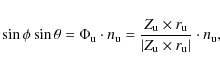
|
(A.2) |
| (A.3) |
The radiation coordinates are defined on the intervals

|
(A.4) |
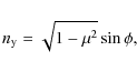
|
(A.5) |
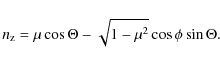
Equations (A.1)-(A.6) are used to update the physical position (
For spherically symmetric wind models, we adhere
to the customary (p,z) spatial coordinate system with p being the
impact parameter and z the direction toward the observer.
Each time a photon is scattered and its direction determined, a new impact parameter is
computed from the relation
![]() ,
appreciating
that all points on a surface of constant radius can be treated equally in this geometry.
,
appreciating
that all points on a surface of constant radius can be treated equally in this geometry.
![\begin{figure}
\par\resizebox{8.5cm}{!}{\includegraphics[angle=90]{12842f13.ps}}
\end{figure}](/articles/aa/full_html/2010/02/aa12842-09/img214.png)
|
Figure A.1: Illustration of the coordinate system, see text. A color version of this figure is available in the web version. |
| Open with DEXTER | |
Releasing photons.
We release photons from the lower boundary uniformly inAbsorption.
The probability of photon absorption is
with the frequency-dependent opacity
| (A.8) |
with
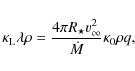
where
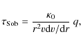
|
(A.10) |
when v and r are expressed in normalized units. The corresponding expression for clumpy winds is provided in Eq. (5). The absorption profile is assumed to be a Gaussian with a Doppler width

and transform to the co-moving frame (hereafter CMF).
![\begin{displaymath}
\Delta \tau_{\nu} = \left\vert\frac{\lambda R_\star}{v_{\in...
...rac{-\Delta \rm erf[\it x_{\rm cmf}/v_{\rm t}]}{2}\right\vert,
\end{displaymath}](/articles/aa/full_html/2010/02/aa12842-09/img238.png)
where
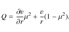
|
(A.13) |
For spherically symmetric winds, we have written a second implementation that allows for line transfer using the Sobolev approximation. With this method each resonance zone is approximated by a point and the line only collects optical depth at atmospheric locations where the observer's frame frequency
Re-emission.
We assume complete redistribution and isotropic re-emission in the CMF, allowing for a multitude of scattering events within one resonance zone. When the Sobolev approximation is applied, re-emission is assumed to be coherent in the CMF and for the angular re-distribution we then use the corresponding escape probabilities (Castor 1970), corrected for a treatment of negative velocity gradients (Rybicki & Hummer 1978; POF). In this case, there is only one effective scattering event inside the localized resonance zone.After the photon has been re-emitted at some atmospheric location, the procedure runs again and searches for another absorption.
A.2 Radiative transfer code tests
![\begin{figure}
\par\includegraphics[width=8.6cm,clip]{12842f14.eps}
\end{figure}](/articles/aa/full_html/2010/02/aa12842-09/img245.png)
|
Figure A.2:
Synthetic line profiles for spherically symmetric
models, calculated with the labeled methods. Profiles are shown
for a smooth model with
|
| Open with DEXTER | |
In this subsection we describe some of the verification tests of our MC radiative transfer code that we have made. The MC-1D version was first applied on spherically symmetric winds, comparing profiles from smooth, stationary winds to profiles calculated using the well-established CMF (cf. Mihalas et al. 1975; Hamann 1981) and SEI methods, and profiles from time-dependent RH winds to profiles calculated using the Sobolev method developed in POF. Thereafter we applied the MC-2D version on models in which all lateral slices had the same radial structure, comparing the results to the MC-1D version.
First we calculated line profiles for smooth, 1D winds. We have verified
that for low![]() values of
values of ![]() ,
profiles from all the methods described above agree perfectly, whereas for
higher values the MC-1D and CMF give identical results but the SEI deviates
significantly, especially for a medium-strong line (see
Fig. A.2, upper panel). This is due to the hybrid nature of
the SEI technique, which approximates the source function with its local
Sobolev value but carries out the exact formal integral. Because of this,
the method does not account for the increasing amount of photons close to
line center that are backscattered into the photosphere when the resonance
zone grows and overlaps with the lower boundary
,
profiles from all the methods described above agree perfectly, whereas for
higher values the MC-1D and CMF give identical results but the SEI deviates
significantly, especially for a medium-strong line (see
Fig. A.2, upper panel). This is due to the hybrid nature of
the SEI technique, which approximates the source function with its local
Sobolev value but carries out the exact formal integral. Because of this,
the method does not account for the increasing amount of photons close to
line center that are backscattered into the photosphere when the resonance
zone grows and overlaps with the lower boundary![]() Consequently the re-emitted flux in this region is higher
when calculated via the SEI than when calculated via the CMF or MC methods.
These discrepancies between the CMF and SEI are quite well documented and
discussed (e.g., Lamers et al. 1987; Hamann 1981), however we still emphasize
that one should exercise caution when applying the SEI method with high
microturbulence on wind resonance lines. Especially today, when increased
computer-power enables us to compute fast solutions using both methods, the
CMF is preferable.
Consequently the re-emitted flux in this region is higher
when calculated via the SEI than when calculated via the CMF or MC methods.
These discrepancies between the CMF and SEI are quite well documented and
discussed (e.g., Lamers et al. 1987; Hamann 1981), however we still emphasize
that one should exercise caution when applying the SEI method with high
microturbulence on wind resonance lines. Especially today, when increased
computer-power enables us to compute fast solutions using both methods, the
CMF is preferable.
Next we calculated line profiles for structured, 1D winds. Profiles computed with all three methods agreed for weak and intermediate lines. For strong lines, the agreement between MCS-1D and the method from POF, which uses a Sobolev source function accounting for multiple-resonance points, was satisfactory. However, minor discrepancies between Sobolev and non-Sobolev treatments occurred for the strong line also when no microturbulent velocity was applied (see Fig. A.2), as opposed to the smooth case.
Finally we performed a simple test of our MC-2D code by applying it on models in which all lateral slices had the same radial structure, i.e., the wind was still spherically symmetric and all observers ought to see the same spectrum. We confirmed that indeed so was the case, both for smooth and structured models (in Fig. A.2 the latter case is demonstrated).
Appendix B: The effective escape ratio
We define the ratio of the velocity gap
|
(B.1) |
In the following, we derive an expression for
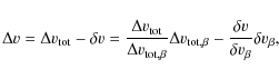
|
(B.2) |
where we have normalized the arbitrary velocity intervals to the corresponding
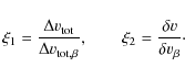
|
(B.3) |
Assuming radial photons,
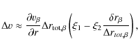
with the notations of r following those of v. The volume filling factor for the geometry in use is
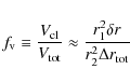
with
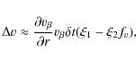
|
(B.6) |
and for
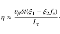
|
(B.7) |
In our models
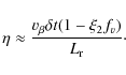
We notice that the porosity length h as defined by Owocki et al. (2004) is
References
- Abbott, D. C., Bieging, J. H., & Churchwell, E. 1981, ApJ, 250, 645 [NASA ADS] [CrossRef] [Google Scholar]
- Bouret, J.-C., Lanz, T., Hillier, D. J., et al. 2003, ApJ, 595, 1182 [NASA ADS] [CrossRef] [Google Scholar]
- Bouret, J.-C., Lanz, T., & Hillier, D. J. 2005, A&A, 438, 301 [NASA ADS] [CrossRef] [EDP Sciences] [Google Scholar]
- Busche, J. R., & Hillier, D. J. 2000, ApJ, 531, 1071 [NASA ADS] [CrossRef] [Google Scholar]
- Castor, J. I. 1970, MNRAS, 149, 111 [NASA ADS] [Google Scholar]
- Castor, J. I., Abbott, D. C., & Klein, R. I. 1975, ApJ, 195, 157 [NASA ADS] [CrossRef] [Google Scholar]
- Crowther, P. A., Hillier, D. J., Evans, C. J., et al. 2002, ApJ, 579, 774 [NASA ADS] [CrossRef] [Google Scholar]
- Dessart, L., & Owocki, S. P. 2002, A&A, 383, 1113 [NASA ADS] [CrossRef] [EDP Sciences] [Google Scholar]
- Dessart, L., & Owocki, S. P. 2003, A&A, 406, L1 [NASA ADS] [CrossRef] [EDP Sciences] [Google Scholar]
- Dessart, L., & Owocki, S. P. 2005, A&A, 437, 657 [NASA ADS] [CrossRef] [EDP Sciences] [Google Scholar]
- Eversberg, T., Lepine, S., & Moffat, A. F. J. 1998, ApJ, 494, 799 [NASA ADS] [CrossRef] [Google Scholar]
- Feldmeier, A. 1995, A&A, 299, 523 [NASA ADS] [Google Scholar]
- Feldmeier, A., Puls, J., & Pauldrach, A. W. A. 1997, A&A, 322, 878 [NASA ADS] [Google Scholar]
- Feldmeier, A., Oskinova, L., & Hamann, W.-R. 2003, A&A, 403, 217 [NASA ADS] [CrossRef] [EDP Sciences] [Google Scholar]
- Fullerton, A. W., Massa, D. L., & Prinja, R. K. 2006, ApJ, 637, 1025 [NASA ADS] [CrossRef] [Google Scholar]
- Gräfener, G., Koesterke, L., & Hamann, W.-R. 2002, A&A, 387, 244 [NASA ADS] [CrossRef] [EDP Sciences] [Google Scholar]
- Hamann, W.-R. 1981, A&A, 93, 353 [NASA ADS] [Google Scholar]
- Hamann, W.-R., Feldmeier, A., & Oskinova, L. M. 2008, Clumping in hot-star winds [Google Scholar]
- Hamann, W., Graefener, G., Oskinova, L. M., & Feldmeier, A. 2009, AIP Conf. Proc., 1171, 136 [NASA ADS] [CrossRef] [Google Scholar]
- Hillier, D. J., & Miller, D. L. 1998, ApJ, 496, 407 [NASA ADS] [CrossRef] [Google Scholar]
- Hirschi, R. 2008, in Clumping in Hot-Star Winds, ed. W.-R. Hamann, A. Feldmeier, & L. M. Oskinova, 9 [Google Scholar]
- Krticka, J., & Kubát, J. 2009, MNRAS, 394, 2065 [NASA ADS] [CrossRef] [Google Scholar]
- Kudritzki, R.-P., & Puls, J. 2000, ARA&A, 38, 613 [NASA ADS] [CrossRef] [Google Scholar]
- Lamers, H. J. G. L. M., Cerruti-Sola, M., & Perinotto, M. 1987, ApJ, 314,726 [NASA ADS] [CrossRef] [Google Scholar]
- Lépine, S., & Moffat, A. F. J. 2008, AJ, 136, 548 [NASA ADS] [CrossRef] [Google Scholar]
- Lucy, L. B. 1983, ApJ, 274, 372 [NASA ADS] [CrossRef] [Google Scholar]
- Lucy, L. B., & Solomon, P. M. 1970, ApJ, 159, 879 [NASA ADS] [CrossRef] [Google Scholar]
- Massa, D. L., Prinja, R. K., & Fullerton, A. W. 2008, in Clumping in Hot-Star Winds, ed. W.-R. Hamann, A. Feldmeier, & L. M. Oskinova, 147 [Google Scholar]
- Meynet, G., Maeder, A., Schaller, G., Schaerer, D., & Charbonnel, C. 1994, A&AS, 103, 97 [NASA ADS] [Google Scholar]
- Mihalas, D., Kunasz, P. B., & Hummer, D. G. 1975, ApJ, 202, 465 [NASA ADS] [CrossRef] [Google Scholar]
- Oskinova, L. M., Feldmeier, A., & Hamann, W.-R. 2004, A&A, 422, 675 [NASA ADS] [CrossRef] [EDP Sciences] [Google Scholar]
- Oskinova, L. M., Feldmeier, A., & Hamann, W.-R. 2006, MNRAS, 372, 313 [NASA ADS] [CrossRef] [Google Scholar]
- Oskinova, L. M., Hamann, W.-R., & Feldmeier, A. 2007, A&A, 476, 1331 [NASA ADS] [CrossRef] [EDP Sciences] [Google Scholar]
- Owocki, S. P. 2008, in Clumping in Hot-Star Winds, ed. W.-R. Hamann, A. Feldmeier, & L. M. Oskinova, 121 [Google Scholar]
- Owocki, S. P., & Rybicki, G. B. 1984, ApJ, 284, 337 [NASA ADS] [CrossRef] [Google Scholar]
- Owocki, S. P., Castor, J. I., & Rybicki, G. B. 1988, ApJ, 335, 914 [NASA ADS] [CrossRef] [Google Scholar]
- Owocki, S. P., Gayley, K. G., & Shaviv, N. J. 2004, ApJ, 616, 525 [NASA ADS] [CrossRef] [Google Scholar]
- Pauldrach, A., Puls, J., & Kudritzki, R. P. 1986, A&A, 164, 86 [NASA ADS] [Google Scholar]
- Pauldrach, A. W. A., Hoffmann, T. L., & Lennon, M. 2001, A&A, 375, 161 [NASA ADS] [CrossRef] [EDP Sciences] [Google Scholar]
- Puls, J., Owocki, S. P., & Fullerton, A. W. 1993, A&A, 279, 457 [NASA ADS] [Google Scholar]
- Puls, J., Urbaneja, M. A., Venero, R., et al. 2005, A&A, 435, 669 [NASA ADS] [CrossRef] [EDP Sciences] [Google Scholar]
- Puls, J., Markova, N., Scuderi, S., et al. 2006, A&A, 454, 625 [NASA ADS] [CrossRef] [EDP Sciences] [Google Scholar]
- Puls, J., Markova, N., & Scuderi, S. 2008a, in Mass Loss from Stars and the Evolution of Stellar Clusters, ed. A. de Koter, L. J. Smith, & L. B. F. M. Waters, ASP Conf. Ser., 388, 101 [Google Scholar]
- Puls, J., Vink, J. S., & Najarro, F. 2008b, A&ARv, 16, 209 [NASA ADS] [CrossRef] [EDP Sciences] [Google Scholar]
- Repolust, T., Puls, J., & Herrero, A. 2004, A&A, 415, 349 [NASA ADS] [CrossRef] [EDP Sciences] [Google Scholar]
- Runacres, M. C., & Owocki, S. P. 2002, A&A, 381, 1015 [NASA ADS] [CrossRef] [EDP Sciences] [Google Scholar]
- Rybicki, G. B., & Hummer, D. G. 1978, ApJ, 219, 654 [NASA ADS] [CrossRef] [Google Scholar]
- Smith, N., & Owocki, S. P. 2006, ApJ, 645, L45 [NASA ADS] [CrossRef] [Google Scholar]
- Vink, J. S., de Koter, A., & Lamers, H. J. G. L. M. 2000, A&A, 362, 295 [NASA ADS] [Google Scholar]
- Zsargó, J., Hillier, D. J., Bouret, J.-C., et al. 2008, ApJ, 685, L149 [NASA ADS] [CrossRef] [Google Scholar]
Footnotes
- ... gas
![[*]](/icons/foot_motif.png)
- We here notice that
 is normalized to the total volume, i.e.,
 .
In some literature
is
identified with the straight volume ratio
.
In some literature
is
identified with the straight volume ratio
 ,
which then implicitly assumes that
,
which then implicitly assumes that
 .
.
- ...
strength
- with
 proportional to the product of mass-loss
rate and abundance of the considered ion, see Appendix A.
proportional to the product of mass-loss
rate and abundance of the considered ion, see Appendix A.
- ... rates
- Recall that
 ,
which implies
,
which implies
 ,
if
,
if
 were derived from
 -diagnostics assuming optically thin clumps.
- ... transfer
- The indirect effect through the feedback on the occupation numbers is not included, because in this section we assume constant ionization.
- ...
wind
- The effect is minor in POF, since these RH models only
extend to
 (see Sect. 2.1).
- ... gradient
- Actually, the velocity gradient may further steepen during advection, due to faster gas trying to overtake slower gas ahead of it; however, this effect is balanced by pressure forces in the subsonic postshock domain.
- ... wind
- This stratification has been
found to be prototypical for O-supergiants and was, together with its well
developed PV P Cygni profiles, the major reason for choosing Cep as
comparison object instead of, e.g.,
 Pup, which displays a somewhat
unusual run of
.
Pup, which displays a somewhat
unusual run of
.
- ... ``infinity''
- The full 3D problem would require binning in
 as well,
which in turn would require a large increase in the number of simulated photons.
as well,
which in turn would require a large increase in the number of simulated photons.
- ... low
- For a typical terminal velocity value
 ,
,
 corresponds to
 and
and
 to
to
 .
.
- ... boundary
- Remember that
neither the SEI nor the CMF, as formulated here, include a transition to the
photosphere, but treat the lower boundary as sharp with a minimum velocity
 .
.
All Tables
Table 1: Basic parameters defining a stochastic wind model clumped in density and with a non-monotonic velocity field.
Table 2: Primary stochastic wind models and parameters.
All Figures
|
|
Figure 1: Left panel: density contour plots of one stochastic (upper plot) and one RH (FPP, lower plot) model. The Cartesian coordinate Z is on the abscissa and X is on the ordinate. Right panel: density and velocity structures of one slice in one stochastic ( upper) and one RH (FPP, lower) model. Over densities are marked with filled dots. For model parameters and details, see Sect. 2.2. |
| Open with DEXTER | |
| In the text | |
| |
Figure 2: Non-monotonic velocity field and corresponding parameters in a stochastic model. |
| Open with DEXTER | |
| In the text | |
|
|
Figure 3:
Synthetic line profiles calculated from 2D RH models. The
abscissa is the dimensionless frequency x (Eq. (A.5)),
normalized to the terminal velocity, and the ordinate is the flux
normalized to the continuum. Upper panel: profiles from
POF models with
|
| Open with DEXTER | |
| In the text | |
|
|
Figure 4:
Left panels: solid lines display total line profiles
and the absorption part for the default stochastic model (see
Table 2), with
|
| Open with DEXTER | |
| In the text | |
|
|
Figure 5: Velocity ( upper panel) and density ( lower panel) structures for one slice in POF (dashed) and RHcopy (dotted), see Table 2. Solid lines are the corresponding smooth structures, and clumps are highlighted as in Fig. 1. |
| Open with DEXTER | |
| In the text | |
|
|
Figure 6:
Left: schematic of |
| Open with DEXTER | |
| In the text | |
|
|
Figure 7:
Equivalent widths
|
| Open with DEXTER | |
| In the text | |
|
|
Figure 8:
Upper: velocity structures (one slice) in
two stochastic models with density-clumping parameters as for the
default model, and different velocity parameters. Dashed:
|
| Open with DEXTER | |
| In the text | |
|
|
Figure 9:
Total, absorption part, and re-emission part line profiles
for 1D, smooth models with
|
| Open with DEXTER | |
| In the text | |
|
|
Figure 10:
Upper panel: density structures of one slice in
the default stochastic model ( upper), in the default stochastic
model with a modified |
| Open with DEXTER | |
| In the text | |
|
|
Figure 11:
Upper: velocity spans of
density enhancements in the FPP model (squares) and corresponding
|
| Open with DEXTER | |
| In the text | |
|
|
Figure 12:
Observed FUSE spectra of the PV doublet
|
| Open with DEXTER | |
| In the text | |
|
|
Figure A.1: Illustration of the coordinate system, see text. A color version of this figure is available in the web version. |
| Open with DEXTER | |
| In the text | |
|
|
Figure A.2:
Synthetic line profiles for spherically symmetric
models, calculated with the labeled methods. Profiles are shown
for a smooth model with
|
| Open with DEXTER | |
| In the text | |
Copyright ESO 2010
Current usage metrics show cumulative count of Article Views (full-text article views including HTML views, PDF and ePub downloads, according to the available data) and Abstracts Views on Vision4Press platform.
Data correspond to usage on the plateform after 2015. The current usage metrics is available 48-96 hours after online publication and is updated daily on week days.
Initial download of the metrics may take a while.