Multi-wavelength properties of Spitzer selected starbursts at z ~ 2

N. Fiolet; A. Omont; M. Polletta; F. Owen; S. Berta; D. Shupe; B. Siana; C. Lonsdale; V. Strazzullo; M. Pannella; A. J. Baker; A. Beelen; A. Biggs; C. De Breuck; D. Farrah; R. Ivison; G. Lagache; D. Lutz; L. J. Tacconi; R. Zylka

doi:10.1051/0004-6361/200912742

Home

All issues

Volume 508 / No 1 (December II 2009)

A&A, 508 1 (2009) 117-132

Full HTML

Free Access

Issue		A&A Volume 508, Number 1, December II 2009


Page(s)		117 - 132
Section		Extragalactic astronomy
DOI		https://doi.org/10.1051/0004-6361/200912742
Published online		15 October 2009

A&A 508, 117-132 (2009)

Multi-wavelength properties of Spitzer selected starbursts at z $\sim$ 2

N. Fiolet^1,2 - A. Omont^1,2 - M. Polletta^1,2,3 - F. Owen⁴ - S. Berta⁵ - D. Shupe⁶ - B. Siana⁷ - C. Lonsdale⁸ - V. Strazzullo⁴ - M. Pannella⁴ - A. J. Baker⁹ - A. Beelen¹⁰ - A. Biggs^11,12 - C. De Breuck¹² - D. Farrah¹³ - R. Ivison^{11, 14} - G. Lagache¹⁰ - D. Lutz⁵ - L. J. Tacconi⁵ - R. Zylka¹⁵

1 - UPMC Univ Paris 06, UMR7095, Institut d'Astrophysique de Paris, 75014 Paris, France
2 - CNRS, UMR7095, Institut d'Astrophysique de Paris, 75014 Paris, France
3 - INAF-IASF Milano, via E. Bassini 15, 20133 Milan, Italy
4 - National Radio Astronomy Observatory, PO Box 0, Socorro, NM 87801, USA
5 - Max-Planck Institut für extraterrestrische Physik, Postfach 1312, 85741 Garching, Germany
6 - Herschel Science Center, California Institute of Technology, 100-22, Pasadena, CA 91125, USA
7 - Astronomy Department, California Institute of Technology, MC 105-24, 1200 East California Boulevard, Pasadena, CA 91125, USA
8 - North American ALMA Science Center, NRAO, Charlottesville, USA
9 - Department of Physics and Astronomy, Rutgers, the State University of New Jersey, 136 Frelinghuysen Road, Piscataway, NJ 08854, USA
10 - Institut d'Astrophysique Spatiale, Université de Paris XI, 91405 Orsay Cedex, France
11 - UK Astronomy Technology Centre, Royal Observatory, Blackford Hill, Edinburgh EH9 3HJ, UK
12 - European Southern Observatory, Karl-Schwarzschild Strasse, 85748 Garching bei München, Germany
13 - Department of Physics & Astronomy, University of Sussex, Falmer, Brighton, BN1 9RH, UK
14 - Institute for Astronomy, University of Edinburgh, Blackford Hill, Edinburgh EH9 3HJ, UK
15 - Institut de Radioastronomie Millimétrique, 300 rue de la Piscine, 38406 St.-Martin-d'Hères, France

Received 22 June 2009 / Accepetd 1 September 2009

Abstract
Context. Wide-field Spitzer surveys allow identification of thousands of potentially high-z submillimeter galaxies (SMGs) through their bright 24 $\mu$ m emission and their mid-IR colors.
Aims. We want to determine the average properties of such $z\sim 2$ Spitzer-selected SMGs by combining millimeter, radio, and infrared photometry for a representative IR-flux ( $\lambda_{\rm rest}\sim 8~\mu$ m) limited sample of SMG candidates.
Methods. A complete sample of 33 sources believed to be starbursts (``5.8 $\mu$ m-peakers'') was selected in the (0.5 deg²) J1046+56 field with selection criteria $F_{\rm 24~\mu m}$ 400 $\mu$ Jy, the presence of a redshifted stellar emission peak at 5.8 $\mu$ m, and $r^\prime_{\rm Vega}$ 23. The field, part of the SWIRE Lockman Hole field, benefits from very deep VLA/GMRT 20 cm, 50 cm, and 90 cm radio data (all 33 sources are detected at 50 cm), and deep 160 $\mu$ m and 70 $\mu$ m Spitzer data. The 33 sources, with photometric redshifts $\sim$ 1.5-2.5, were observed at 1.2 mm with IRAM-30m/MAMBO to an rms $\sim$ 0.7-0.8 mJy in most cases. Their millimeter, radio, 7-band Spitzer, and near-IR properties were jointly analyzed.
Results. The entire sample of 33 sources has an average 1.2 mm flux density of $1.56 \pm 0.22$ mJy and a median of 1.61 mJy, so the majority of the sources can be considered SMGs. Four sources have confirmed 4 $\sigma$ detections, and nine were tentatively detected at the 3 $\sigma$ level. Because of its 24 $\mu$ m selection, our sample shows systematically lower $F_{\rm 1.2~mm}/F_{\rm 24~\mu m}$ flux ratios than classical SMGs, probably because of enhanced PAH emission. A median FIR SED was built by stacking images at the positions of 21 sources in the region of deepest Spitzer coverage. Its parameters are $T_{\rm dust} = 37 \pm 8$ K, $L_{\rm FIR} = 2.5 \times 10^{12}~L_{\odot}$ , and SFR = 450 $M_{\odot }$ yr^-1. The FIR-radio correlation provides another estimate of $L_{\rm FIR}$ for each source, with an average value of $4.1 \times 10^{12}~L_{\odot}$ ; however, this value may be overestimated because of some AGN contribution. Most of our targets are also luminous star-forming BzK galaxies which constitute a significant fraction of weak SMGs at $1.7 \lesssim z \lesssim 2.3.$
Conclusions. Spitzer 24 $\mu$ m-selected starbursts and AGN-dominated ULIRGs can be reliably distinguished using IRAC-24 $\mu$ m SEDs. Such ``5.8 $\mu$ m-peakers'' with $F_{\rm 24~\mu m}$ 400 $\mu$ Jy have $L_{\rm FIR}~\gtrsim 10^{12}~L_{\odot}$ . They are thus $z\sim 2$ ULIRGs, and the majority may be considered SMGs. However, they have systematically lower 1.2 mm/24 $\mu$ m flux density ratios than classical SMGs, warmer dust, comparable or lower IR/mm luminosities, and higher stellar masses. About 2000-3000 ``5.8 $\mu$ m-peakers'' may be easily identifiable within SWIRE catalogues over 49 deg².

Key words: galaxies: high-redshift - galaxies: starburst - galaxies: active - infrared: galaxies - submillimeter - radio continuum: galaxies

1 Introduction

Ultra-Luminous InfraRed Galaxies (ULIRGs, with $L_{\rm FIR} \gtrsim 10^{12}~L_{\odot}$ ) are the most powerful class of star-forming galaxies. For 25 years, these prominent sources and their intense starbursts have been the target of many comprehensive studies, both locally (e.g., Sanders & Mirabel 1996; Lonsdale et al. 2006; Veilleux et al. 2009) and at high redshift (e.g., Solomon & Vanden Bout 2005; Blain et al. 2004). While local ULIRGs are relatively rare, submm/mm surveys with large bolometer arrays such as JCMT/SCUBA (James Clerk Maxwell Telescope/Submillimetre Common User Bolometer Array, Holland et al. 1999), APEX/LABOCA (Atacama Pathfinder Experiment/Large Apex Bolometer Camera, Siringo et al. 2009) or IRAM/MAMBO (Institut de Radioastronomie Millimétrique/Max-Planck Bolometer Array, Kreysa et al. 1998) have shown that the comoving density of submillimetre galaxies (SMGs), which represent a significant class of high-redshift ( $z\sim1{-}4$ ) ULIRGs, is about a thousand times greater than that of ULIRGs in the local Universe (e.g., Chapman et al. 2005; Le Floc'h et al. 2005). They represent a major phase of star formation at early epochs and are also characterized by high stellar masses (e.g., Borys et al. 2005). They are thus ideal candidates to be the precursors of local massive elliptical galaxies (e.g., Blain et al. 2002; Lonsdale et al. 2009; Dye et al. 2008, hereafter Lo09, and references therein). Nearly all of the enormous UV energy produced by their massive young stars is absorbed by interstellar dust and re-emitted at far-infrared wavelengths, with their far-infrared luminosity ( $L_{\rm FIR}$ ) able to reach $10^{13}~L_{\odot}$ . However, despite the considerable efforts invested in mm/submm surveys, the total number of known SMGs remains limited to several hundred, and current observational capabilities are still somewhat marginal at many wavelengths. We thus still lack comprehensive studies of SMGs and their various subclasses at all wavelengths and redshifts and in various environments. Even their star formation rates (SFRs) remain uncertain in most cases because of a lack of direct observations at the FIR/submm wavelengths of their maximum emission. The identification of large samples of SMGs is important for investigating the properties of these galaxies (SFR, luminosity, spectral energy distribution [SED], stellar mass, AGN content, spatial structure, radio and X-ray parameters, clustering, etc.) on a statistical basis, as a function of their various subclasses, redshift, and environment. This is the main goal of the wide-field submm surveys planned with SCUBA2 and Herschel.

Although Spitzer generally lacks the sensitivity to detect SMGs in the far-IR, its very good sensitivity in the mid-IR allows the efficient detection of a significant fraction of SMGs in the very large area observed by its wide-field surveys, and in particular the $\sim$ $49~\rm {deg}^2$ Spitzer Wide-area Infrared Extragalactic (SWIRE) survey (Lonsdale et al. 2003). From an analysis of a sample of $\sim$ 100 SMGs observed with Spitzer, Lo09 have estimated that SWIRE has detected more than 180 SMGs with $F_{\rm 1.2~mm} > 2.5~$ mJy per square degree at 24 $\mu$ m and in several IRAC bands from 3.6 to 8.0 $\mu$ m. However, the identification of SMGs among SWIRE sources is not straightforward, since it requires inferring FIR emission from mid-IR photometry in objects with various SEDs, especially as regards AGN versus starburst emission, and various redshifts.

$\begin{figure} \par\resizebox{8.5cm}{!}{\includegraphics{12742f1.eps}} \end{figure}$

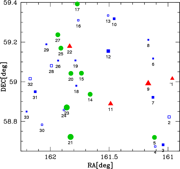
Figure 1:

Positions of the 33 sources of our sample ( $42^\prime \times 42^\prime$ J1046+59 field, centred at the VLA position observed by Owen & Morrison (2008), $\alpha _{2000}=10$ h46m00s, $\delta_{2000}=+59\degr01\hbox{$^\prime$ }00\hbox{$^{\prime\prime}$ }$ ). The red filled triangles are the $4\sigma$ detections at 1.2 mm. The green filled circles are the $3\sigma$ tentative detections at 1.2 mm. The blue squares are sources with a signal at 1.2 mm lower than $3\sigma$ . The sizes of symbols are proportional to 1.2 mm strengths. The open symbols show no detection at 20 cm (Owen & Morrison 2008).

Open with DEXTER

We have therefore undertaken a systematic study of the 1.2 mm emission from the best SMG candidates among Spitzer bright 24 $\mu$ m sources, focusing on $z~\sim$ 2 starburst candidates. In Lonsdale et al. (2006) and Lo09 (see also Farrah et al. 2008; Weedman et al. 2006), it is shown that selecting sources with a secondary maximum emission in one of the intermediate IRAC bands at 4.5 or 5.8 $\mu$ m provides an efficient discrimination against AGN power-law SEDs. In particular, 24 $\mu$ m bright ``5.8 $\mu$ m-peakers'' have a high probability of being dominated by a strong starburst at $z\sim 2$ , whose intense 7.7 $\mu$ m feature is redshifted into the 24 $\mu$ m band. A first 1.2 mm MAMBO study of a sample of $\sim$ 60 bright SWIRE sources (Lo09) has confirmed that such a selection yields a high detection rate at 1.2 mm and a significant average 1.2 mm flux density, showing that the majority of such sources are high-z ULIRGs, probably at $z\sim 2$ . However, as described in Lo09, this sample was selected with the aim of trying to observe the ``5.8 $\mu$ m-peakers'' with the strongest mm flux over more than 10 deg². This was achieved by deriving photometric redshifts, estimating the expected 1.2 mm flux densities by fitting templates of various local starbursts and ULIRGs to the optical and infrared (3.6-24 $\mu$ m) bands, and selecting the candidates predicted to give the strongest mm emission. Therefore, the selection criteria of this sample were biased, especially toward the strongest 24 $\mu$ m sources and those in clean environments. We report here the results of an analogous MAMBO study, but of a complete 24 $\mu$ m-flux limited sample of all SWIRE ``5.8 $\mu$ m-peakers'' in a 0.5 deg² region within the SWIRE Lockman Hole field, with $F_{\rm 24~\mu m} > 400~\mu$ Jy and $r^\prime_{\rm Vega} > 23$ (see Sect. 2 for a precise definition of ``5.8 $\mu$ m-peakers'', which of course depends on the actual SWIRE data and limits of sensitivity and accuracy). This region was selected because of the richness in multi-wavelength data, in particular the exceptionally deep radio data at 20 cm (VLA, Owen & Morrison 2008), 50 cm (GMRT, Owen et al. in prep.), and 90 cm (VLA, Owen et al. 2009). Our study aims at characterizing the average multi-wavelength properties of these sources, their dominant emission processes (starburst or AGN), their stellar masses, and their star formation rates. We adopt a standard flat cosmology: H₀=71 km s^-1 Mpc^-1, $\Omega_{\rm M}=0.27$ and $\Omega_{\Lambda}=0.73$ (Spergel et al. 2003).

2 Sample selection and ancillary data

We selected all Spitzer/SWIRE ``5.8 $\mu$ m-peakers'' with $F_{\rm 24~\mu m} > 400~\mu$ Jy in the $42^\prime \times 42^\prime$ (0.49 deg²) J1046+59 field in the SWIRE Lockman Hole, centered at $\alpha _{2000}=10$ h46m00s, $\delta_{2000}=+59\degr01\hbox{$^\prime$ }00\hbox{$^{\prime\prime}$ }$ (Fig. 1). A source is considered to be a ``5.8 $\mu$ m-peaker'' if it satisfies the following conditions: $F_{\rm 3.6~\mu m} < F_{\rm 4.5~\mu m} < F_{\rm 5.8~\mu m} > F_{\rm 8.0~\mu m}$ , without consideration of uncertainties. 13 sources have no detection in the 8.0 $\mu$ m band. We assume that these sources are also ``5.8 $\mu$ m-peakers'' because their fluxes at 5.8 $\mu$ m are greater than the detection limits at 8.0 $\mu$ m ( 40 $\mu$ Jy). We also require that the sources are optically faint, i.e., $r^\prime_{\rm Vega} > 23$ , to remove low redshift interlopers (Lonsdale et al. 2006). The selected sample contains 33 sources, which represent 6% of all sources with $F_{\rm 24~\mu m} > 400~\mu$ Jy and $r^\prime_{\rm Vega} > 23$ in the field.

We use the SWIRE internal catalogue available at the time of definition of the project, September 2006. Details on the SWIRE observations and data are available in Surace et al. (2005). The 2006 SWIRE internal catalogue has been superseded by the current version, dated 2007. Since our selection, MAMBO observations, and analysis were based on the 2006 catalogue, but there are no significant changes for our sources in the 2007 catalogue, and the numbers of sources selected in the two versions of the catalogue do not vary significantly, for this work we will use the selection from 2006 data. Based on the analysis of the sources that would have been missed or included applying our selection criteria to the two versions of the catalogues, we find that the original sample selected from the 2006 SWIRE catalogue remains representative of a sample strictly meeting our selection criteria.

We have reported in Table 1 the fluxes from the 2006 SWIRE catalogue. The optical magnitudes have been obtained with the MOSAIC camera on the 4-m Mayall Telescope at Kitt Peak National Observatory (e.g., Muller et al. 1998). However, for a few sources, the optical data differ slightly from those available in the SWIRE catalogue because a measurement at each source position was performed for all non-detections in the catalogue. The revised optical magnitudes are listed in Table 1.

Table 1: Optical, Near-IR and Spitzer mid-IR data of the selected sample.

Table 2: Related Spitzer-selected $z\sim 2$ ULIRGs samples.

The imaging in the central 0.3 deg² is much deeper (by $\sim$ 0.7 mag). Exact depths are listed in Polletta et al. (2006). In addition to the SWIRE data, we obtained near-infrared (NIR) data from two sources: 1) from Palomar/WIRC (Wilson et al. 2003); 2) from UKIRT/WFCAM (Henry et al. 2000) in the J ( $\lambda$ = 1.25 $\mu$ m), H ( $\lambda$ = 1.63 $\mu$ m), and K( $\lambda$ = 2.20 $\mu$ m) bands as part of a NIR survey of the field. A description of these data and their reduction will be published in Strazzullo et al., in prep. The NIR data are reported in Table 1. 23 sources are detected in all three bands. 24 sources are detected at least in the K-band. The WFCAM K band data are public data from UKIDSS (Warren et al. 2007; Lawrence et al. 2007). Pipeline processing and the science archive are described by Hambly et al. (2008) and Irwin et al. (in prep.).

Table 2 compares the selection criteria for our sample to those for similar samples of bright 24 $\mu$ m sources. The sample of Lo09 is based on the same criteria, but is biased toward sources brighter at 24 $\mu$ m, with 819 $\mu$ Jy on average vs. 566 $\mu$ Jy for the present sample. The sample of Farrah et al. (2008) is similar but aimed at ``4.5 $\mu$ m-peakers''; the sample of Huang et al. (2009) and Younger et al. (2009) is based on different IRAC criteria, but they indeed select almost exclusively ``5.8 $\mu$ m-peakers'' (Sect. 5.1). On the other hand, the selection criteria of Magliocchetti et al. (2007) and Yan et al. (2005), which do not use the IRAC flux densities, do not discriminate against AGN and yield a large proportion of AGN.

Compared to the twin starburst sample of Lo09, the present sample is complete down to a 24 $\mu$ m flux density of 400 $\mu$ Jy. It thus includes weaker 24 $\mu$ m sources on average, but it should be free from the selection biases present in the Lo09 sample that resulted from the effort to maximize the number of detections at 1.2 mm. In addition, our sample benefits from very deep radio data at 1400, 610, and 324 MHz (Sect. 4.3). The positions of the sources in the field are shown in Fig. 1. The radio flux densities are listed in Table 4.

3 MAMBO observations and results

Observations were made during the winter 2006/2007 MAMBO observing pool between December 2006 and March 2007 at the IRAM 30 m telescope, located at Pico Veleta, Spain, using the 117-element version of the MAMBO array (Kreysa et al. 1998) operating at 1.2 mm (250 GHz). We used a standard ``on-off'' photometry observing mode with a secondary mirror wobbling at a frequency of 0.5 Hz between the source and a blank sky position offset in azimuth by $\sim$ $35\hbox{$^{\prime\prime}$ }$ . Periodically, the telescope was nodded so that the sky position lay on the other side of the source position. Pointing and focus were updated regularly on standard sources. Nearly every hour, the atmospheric opacity was measured by observing the sky at six elevations. Our observations are divided in 16 or 20 ``subscans'' of 60 s each. In this operating mode, the integration time is $\sim$ 40 s (20 s on source and 20 s on sky) per subscan. Observations of each source were never concentrated in a single night, but distributed over several nights in order to reduce the risks of systematic effects. The initial aim was to observe the 32 sources (L-12 was observed in the project described by Lo09, under the name ``LH-11'') with an rms $\sim$ 0.8 mJy, which corresponds to $\sim$ 0.6 h of integration for the system sensitivity $\sim$ 35-40 mJy s^-1/2 in average weather conditions. As seen in Table 4, this was achieved for most of the sources. However, for $\sim$ 20% of the sources the rms was instead $\sim$ 0.9-1.1 mJy, while a similar number of sources were observed somewhat longer to reach an rms $\sim$ 0.5-0.6 mJy in order to confirm their detection.

The data reduction is straightforward thanks to the MOPSIC software package, which is regularly updated on the MAMBO pool page. This program reduces the noise due to the sky emission if it is sufficiently correlated between the different bolometers. This process is generally sufficient for the majority of observations. However, in a few cases, some scans may present faults due, e.g., to lack of helium in the cryostat or problems of acquisition. These scans are validated or rejected after close inspection.

The results of our observations at 1.2 mm are reported in Table 4. The average flux density (with equal weight) of the entire sample is $1.56 \pm 0.22$ mJy, very comparable to Lo09 ( $1.49 \pm 0.18$ mJy) and Younger et al. (2009) ( $1.6 \pm 0.1$ mJy), but greater than obtained by Lutz et al. (2005) for a Spitzer-selected sample of high-z starbursts and (mostly) AGNs ( $0.74 \pm 0.09$ mJy). The median for our sample is 1.61 mJy. This confirms that on average the majority of these sources are SMGs (at $z\sim 2$ , 1.6 mJy corresponds to $\sim$ 4 mJy at 850 $\mu$ m: Greve et al. 2004). Because of the limited integration time, only four sources were solidly detected at >4 $\sigma$ . However, the fraction of sources at least tentatively detected at >3 $\sigma$ is 39% (13/33 sources). It is worth stressing that the reliability of such $3\sigma$ tentative detections in careful ``on-off'' MAMBO observations is much higher than those detected in a mm/submm map amongst hundreds of possible resolution elements, where flux boosting is inevitable.

This on-off $3\sigma$ ``detection'' rate is similar to what was obtained by Lo09 for a similar sample, higher than obtained by Lutz et al. (2005) for their Spitzer-selected sample of starbursts and (mostly) AGNs (18%), and lower than obtained by Younger et al. (2009) with deeper observation of a similar sample of Spitzer-selected $z\sim 2$ starbursts (75%).

4 Source properties

4.1 Spectral energy distributions and redshifts

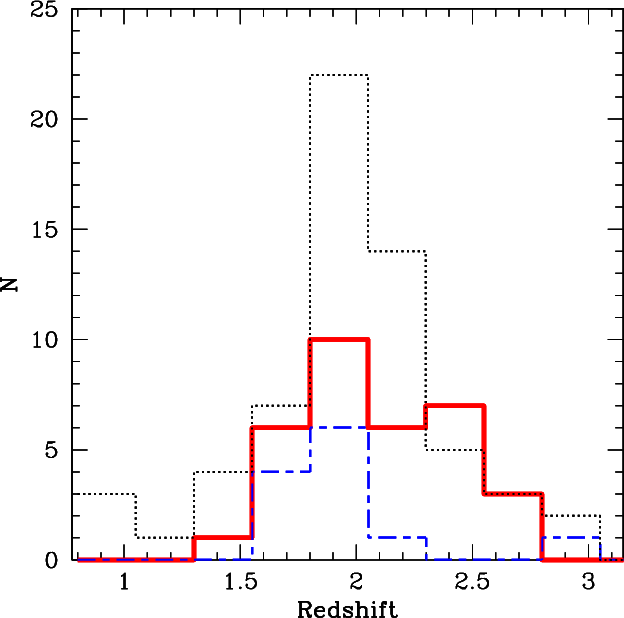
$\begin{figure} \par\resizebox{8.8cm}{!}{\includegraphics{12742f2.eps}} \end{figure}$	Figure 2: Histogram of redshifts for our sample (photometric, thick solid red line), the full sample from Lo09 (photometric and spectroscopic, dotted black line), and the sample from Younger et al. (2009) (spectroscopic, long-short-dashed blue line).
Open with DEXTER

In order to estimate photometric redshifts, we fit the spectral energy distributions (SEDs), including optical and IR ( $\le$ $24~\mu$ m) data for each source, with a library of galaxy templates following the method described in Lo09 and Polletta et al. (2007). The SEDs are fitted using the Hyper-zcode (Bolzonella et al. 2000), and the effects of dust extinction are taken into account. As discussed in Lo09, such photometric redshifts are limited in accuracy and have uncertainties of $\pm$ 0.5.

SED fits for all the sources in the sample are shown in the Appendix (only in the electronic edition), and the photometric redshifts are listed in Table 4. The photometric redshift distribution of the sample is shown in Fig. 2. All redshifts but four are within the range $1.5 \lesssim z \lesssim 2.5$ . The average redshift from these SEDs is $\langle z\rangle = 2.08$ (median = 2.04, scatter = 0.32, and semi-inter-quartile range = 0.26). This result is consistent with our selection criteria, which assume that the 7.7 $\mu$ m PAH band is redshifted into the 24 $\mu$ m MIPS band and the 1.6 $\mu$ m stellar band into the 5.8 $\mu$ m IRAC band. The redshift distribution of our sample is similar to the one measured in Lo09 ( $\langle z \rangle = 1.97 \pm 0.05$ ), which is mostly based on photometric redshifts, and the one measured in Younger et al. (2009) ( $\langle z\rangle = 1.96 \pm 0.10$ ), which is based on spectroscopic redshifts (Fig. 2). Thus, all these works select sources in a similar redshift range. Indeed, the actual redshift distribution of our sample might be similar to that of Huang et al. (2009) and Younger et al. (2009) and concentrated within a rather narrow redshift range around $z\sim 1.7$ -2.3 as shown by the few spectroscopic redshifts reported for the sample of Lo09.

Twelve sources from our sample have redshifts from the catalogue of SWIRE photometric redshifts of Rowan-Robinson et al. (2008). For ten of these sources, our photometric redshifts determined by the SED fitting show a good ( $\pm$ $10\%$ ) agreement with the determinations from Rowan-Robinson et al. (2008).

4.2 Comparison between 1.2 mm and 24 $\mu$ m flux densities

$\begin{figure} \par\resizebox{8.8cm}{!}{\includegraphics{12742f3.eps}} \end{figure}$

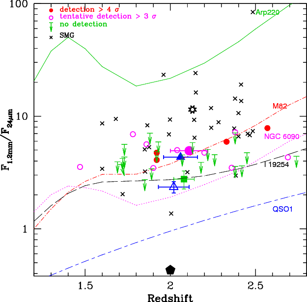
Figure 3:

Observed MAMBO 1.2 mm flux density as a function of 24 $\mu$ m flux density. The black squares show the average flux densities for the first $F_{\rm 24~\mu m}$ quartile (8 sources) and for the 25 other sources, respectively. The filled (open) red circles are the sources that are $4\sigma$ detections ( $3\sigma$ tentative detections) at 1.2 mm. The green arrows are 2 $\sigma$ upper limits for the sources that are not detected at 1.2 mm.

Open with DEXTER

In order to investigate whether there is a correlation between mid-IR and mm emission, we compare the flux densities at 1.2 mm and at 24 $\mu$ m ( $F_{\rm 1.2~mm}$ and $F_{\rm 24~\mu m}$ ) in Fig. 3. Because of the limited sensitivity of the 1.2 mm data, we have stacked the data for the first $F_{\rm 24~\mu m}$ quartile (8 sources), and independently for the 25 other sources. These stacked values have been computed with the observed $F_{\rm 1.2~mm}$ values. Figure 3 shows that it is impossible to see whether there is a correlation between mid-IR and mm emission with this sensitivity. However, the average for the highest $F_{\rm 24~\mu m}$ quartile seems $\sim$ 1.5-2 times larger than the average for all the other sources.

Because of the 24 $\mu$ m selection, the $F_{\rm 1.2~mm}/F_{\rm 24~\mu m}$ ratio of our sources is relatively low compared to that submm selected SMGs, as in the case of Lo09. The ratio of the average $F_{\rm 1.2~mm}$ to the average $F_{\rm 24~\mu m}$ is $2.76 \pm 0.50$ for the entire sample of 33 sources (and $4.94 \pm 0.51$ for 13 sources with 1.2 mm S/N > 3, see Table 3). As seen in Fig. 8, these ratios of averages are a factor $\sim$ 4 ( $\sim$ 2) smaller than that of a sample of literature SMGs (Sect. 5.2), and a factor $\sim$ 6 ( $\sim$ 10) larger than one of the (AGN dominated) sample of bright 24 $\mu$ m sources of Lutz et al. (2005). They are a factor $\sim$ 10 ( $\sim$ 5) smaller than that of the extreme SMG template Arp 220 at z=2, but comparable to those of starburst templates (M 82 or NGC 6090) and AGN-starburst composites (IRAS19254-7245 South).

4.3 Radio properties and the nature of the sources

The studied sources benefit from exceptionally deep VLA data at 1.4 GHz (rms = 2.7 $\mu$ Jy in the center of the field, 12-15 $\mu$ Jy in most of the 0.5 deg² field; Owen & Morrison 2008). Such a depth yields radio detections for almost the entire sample. 8 of 33 sources are not detected due to a loss of radio sensitivity in the outer parts of the field, largely due to the decrease in primary beam sensitivity and bandwidth smearing. The GMRT 610 MHz observations are also very deep (rms = 10 $\mu$ Jy), cover almost the entire field, and detect all 33 sources. The VLA 324 MHz observations reach a depth of rms = 70 $\mu$ Jy and cover the entire field (Owen et al. 2009). They yield detections for 17 sources. The radio flux densities are listed in Table 4. The cross identification was made by comparing the radio and the SWIRE positions. Following the method of Ivison et al. (2007) and Downes et al. (1986), we have verified that all our sources have very reliable radio associations, with an average probability of spurious association in 2 $\hbox{$^{\prime\prime}$ }$ of $\langle P\rangle$ = 0.001. For Ivison et al. (2007), the association is reliable if $P \leq 0.05$ .

Based on the correlation between $L_{\rm FIR}$ and the radio luminosity in star-forming regions and in local starburst galaxies (Sanders & Mirabel 1996; Crawford et al. 1996; Helou et al. 1985; Condon 1992), the radio and FIR luminosities are expected to be linked as well at $z\sim 2$ (Ibar et al. 2008). We discuss this in Sect. 4.4, together with the derivation of $L_{\rm FIR}$ . However, if this correlation is verified at $z\sim 2$ , one may expect a straightforward relation between the radio and 1.2 mm flux densities for starbursts with similar SEDs. To check that, we plot the 1.2 mm flux density as a function of the radio flux density at 20 cm in Fig. 4. Because of the limited sensitivity at 1.2 mm, we consider average values of 1.2 mm flux density and radio flux density, for the entire sample, for the 13 sources with 1.2 mm S/N > 3, and for the 20 sources with 1.2 mm S/N < 3 (Table 3). In Fig. 4, we also report the ratio of the average flux densities and $1\sigma$ dispersion found by Chapman et al. (2005) (see also e.g. Smail et al. 2002; Yun & Carilli 2002; Condon 1992; Ivison et al. 2002) for a sample of radio-detected sub-millimeter galaxies at $z\sim 2$ . The mm/radio ratios for both the whole sample and the S/N > 3 sources are reasonably compatible with the correlation between mm/submm and radio fluxes found for $z\sim 2$ starbursts (Chapman et al. 2005). However, the ratio between average values of 1.2 mm flux density and radio flux density, for the entire sample and especially for the 20 sources with 1.2 mm S/N < 3, might be slightly smaller compared to submm selected galaxies. This could be explained as an effect of the 24 $\mu$ m selection, and by a greater AGN contribution and/or hotter dust (see Sects. 5.3 and 5.4 for a complete discussion).

In order to assess whether the radio emission observed in our sources is associated with AGN or with star-forming regions, one may also consider the radio spectral shape, the rest-frame radio luminosity, and the radio morphology (see e.g. Seymour et al. 2008; Biggs & Ivison 2008). The radio spectral index $\alpha$ , where $F_{\nu}\propto \nu^{\alpha}$ , is first calculated from the flux densities at 20 cm, 50 cm, and 90 cm, when they are available, using the best power law fit between these three wavelengths, and is reported in Table 4. When only two radio fluxes are available, the index is just derived from the flux density ratio. Seven sources have no determined spectral radio index because of a lack of radio detections at 1.4 GHz and 324 MHz.

Most of our sources have a radio spectral index in the range $\sim$ -0.4 to -1.2 (average $\langle \alpha\rangle=-0.64\pm0.07$ ; median = -0.74). This is not very discriminating since, considering the uncertainties, such values of $\alpha$ are typical for star-forming galaxies, type II AGN, and many radio galaxies (e.g., De Breuck et al. 2000; Ciliegi et al. 2003; Polletta et al. 2000; De Breuck et al. 2001; Condon 1992). About 20% of the sources, mostly among those with some radio excess, could either be in the same range or have $\alpha$ $\gtrsim$ -0.5 typical of flat spectrum sources.

$\begin{figure} \par\resizebox{8.8cm}{!}{\includegraphics{12742f4.eps}} \end{figure}$

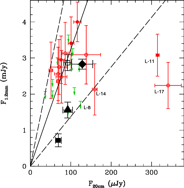
Figure 4:

Observed MAMBO 1.2 mm flux density as a function of 20 cm flux density. The large black symbols show different stacked values: the entire sample (filled triangle), all sources with > $3\sigma$ (filled diamond), the sources with > $3\sigma$ signal without the two strongest radio sources (open square), and the sources with <3 $\sigma$ signal (filled square). The filled (open) red circles are the sources that are $4\sigma$ detections ( $3\sigma$ tentative detections) at 1.2 mm. The green arrows are 2 $\sigma$ upper limits for the sources with S/N < 3 at 1.2 mm. The solid black line shows the correlation derived from Chapman et al. (2005) for $z\simeq 2$ (assuming $F_{\rm 850~\mu m}/F_{\rm 1.2~mm} = 2.5$ at $z\sim 2$ ). The dashed lines are the limits of this correlation at $\pm$ $1\sigma$ . The labelled sources are those with the highest 20 cm/1.2 mm flux density ratios (see Table 4).

Open with DEXTER

Table 3: Derived values from the stacked flux densities^a.

Table 4: 1.2 mm and radio data.

Table 5: Luminosities and star formation rates.

The radio luminosity and the FIR-radio correlation are most often expressed in term of the rest-frame luminosity at 1.4 GHz, $L_{\rm {1.4~GHz}}$ . With the same assumptions as for the SMG sample of Kovács et al. (2006), we can rewrite their Eq. (7) as

$\begin{displaymath}L_{\rm 1.4~GHz}({\rm W~Hz^{-1}})=4\pi D_{\rm L}^{2}F_{\rm 20~cm} (1+z)^{(-\alpha-1)} \end{displaymath}$

(1)

where $D_{\rm L}$ is the luminosity distance. In cases with detections at at least two radio wavelengths, we assume the derived value of $\alpha$ . When only $F_{\rm {50~cm}}$ is available, we assume a fixed $\alpha$ value equal to the average value found for our sample, $\langle \alpha\rangle =-0.64$ .

Using the flux at 610 MHz, this equation becomes

$\begin{displaymath}L_{\rm 1.4~GHz}({\rm W~Hz^{-1}})=4\pi D_{\rm L}^{2}F_{\rm 50~cm}\left(\frac{2.3}{1+z}\right)^{\alpha}\frac{1}{1+z}\cdot \end{displaymath}$

(2)

Finally, we examine the radio sizes of our sources. A large size ( $\gtrsim1\hbox{$^{\prime\prime}$ }$ ) may indicate radio jets or lobes associated with the presence of a radio loud AGN. However, it is also possible that the extended radio emission is associated with star-forming regions distributed across the galaxy, as is the case for some local ULIRGs (e.g., Murphy et al. 2001) and a large fraction of classical SMGs, e.g., $\sim$ 70% in Chapman et al. (2004) (see also Seymour et al. 2008; Richards et al. 2007; Biggs & Ivison 2008). Nine sources are extended (major axis $\gtrsim$ 5 kpc) in the VLA 20 cm images, with most sizes $\gtrsim$ 10 kpc, and the remainder are either unresolved or not detected (see Table 4). The radio luminosities of the nine extended sources range from $\sim$ 10^23.9 W Hz^-1 to $\sim$ 10^24.6 W Hz^-1.

4.4 Far-infrared luminosity

Estimates of $L_{\rm FIR}$ for our individual sources are quite uncertain due to the lack of data between 24 $\mu$ m and 1.2 mm, where most of the far-infrared energy is emitted. None of our sources are detected at 70 $\mu$ m or 160 $\mu$ m at the SWIRE sensitivities (the 3 $\sigma$ limits at 70 and 160 $\mu$ m are 18 and 108 mJy, respectively). There are not even detections in the $\sim$ 2.5 times deeper MIPS images available from GO Program 30391 (PI: Owen) in the center of the field, which is well observed at 20 cm. We thus make use of these deep MIPS data only for stacking the 70 and 160 $\mu$ m images to constrain the average $L_{\rm FIR}$ of our sample.

We estimate average flux densities from the stacked MIPS images at 24, 70, and 160 $\mu$ m, following the method described in Lo09. An initial stack based on the SWIRE MIPS images was made for the entire sample of 33 sources, but it yields only a marginally significant ( $\sim$ 2-3 $\sigma$ ) detection at 160 $\mu$ m. The average flux densities at 70 $\mu$ m and 160 $\mu$ m are almost 5 times lower than the SWIRE 3 $\sigma$ limits (Table 6). We thus use stacks made with the GO-30391 images of the 21 sources covered by these deeper MIPS observations. The results from stacks are reported in Table 6. In addition to the stacked flux densities for the entire sample, we also report stacked flux densities for two subsamples apiece: 10 sources with 1.2 mm SNR > 3, and 11 sources with SNR < 3.

The median stacked flux densities at 70 $\mu$ m and 160 $\mu$ m for the entire sample are quite faint, about 3 mJy and 13 mJy respectively. We use these median stacked flux densities in the following analysis. There is no appreciable difference in $\langle F_{\rm 160~\mu m}\rangle$ and $\langle F_{\rm 70~\mu m\rangle}$ between sources tentatively detected (>3 $\sigma$ ) and undetected (<3 $\sigma$ ) at 1.2 mm. The median 160 $\mu$ m and 70 $\mu$ m flux densities seem smaller than for the previous similar sample of Younger et al. (2009), which has higher average 24 $\mu$ m flux density (Table 6).

We combine the median flux densities at 70 $\mu$ m, 160 $\mu$ m, and 1.2 mm to build a median far-IR SED for our sample. We fit the median FIR SED assuming the average redshift of the sample (z = 2.08) with a ``graybody'' model with a fixed value of the emissivity index ( $\beta = 1.5$ , see e.g. Kovács et al. 2006; Beelen et al. 2006) to derive the temperature, $T_{\rm dust}$ , of a single dust component. The best-fit value for the whole sample is $T_{\rm dust} = 37 \pm 8~$ K. This model yields $L_{\rm FIR} = 2.5 \times 10^{12}~L_{\odot}$ , which is well in the ULIRG range and may be considered the average value for ``5.8 $\mu$ m-peakers'' with $F_{\rm 24~\mu m} > 400~\mu$ Jy and r > 23. Note that these values for $T_{\rm dust}$ and $\langle L_{\rm FIR}\rangle$ are slightly smaller than the values of Lo09, $T_{\rm dust} = 41$ K and $\langle L_{\rm FIR}\rangle = 4.6 \times 10^{12}~L_{\odot}$ and of Younger et al. (2009), $T_{\rm dust} = 41~$ K and $\langle L_{\rm FIR}\rangle = 3.8 \times 10^{12}~L_{\odot}$ .

The actual $L_{\rm FIR}$ of our sources will span some range around this value. Although it is not possible to derive accurate values of $L_{\rm FIR}$ for each source in the absence of individual detections at 160 $\mu$ m or at another wavelength close to the FIR maximum of the SED, several alternative approaches are possible for estimating individual $L_{\rm FIR}$ .

One can simply infer $L_{\rm FIR}$ from the flux density at 1.2 mm, $F_{\rm 1.2~mm}$ . The value of $F_{\rm 1.2~mm}$ can place strong constraints on $L_{\rm FIR}$ if we assume that the whole $L_{\rm FIR}$ and the radiation detected at 1.2 mm are produced by dust heated by the same mechanism. The relation between $L_{\rm FIR}$ and $F_{\rm 1.2~mm}$ can be derived assuming a thermal spectral model. A ``graybody'' model, with a single dust component and emissivity index, e.g. $\beta = 1.5$ (Beelen et al. 2006), yields:

$\begin{displaymath}L_{\rm FIR}(L_{\odot})=\kappa\times10^{12}~F_{\rm 1.2~mm}({\rm mJy}) \end{displaymath}$

(3)

where the proportionality factor, $\kappa \sim 1{-}5$ , depends mainly on $T_{\rm dust}$ but also by a factor of a few on redshift. For redshifts $\sim$ 2, $\kappa = 1.3$ for $T_{\rm dust} = 35~$ K and $\kappa = 2.14$ for $T_{\rm dust} = 40~$ K. The dust temperature, $T_{\rm dust}$ , is difficult to constrain without observations in the FIR-submm range, e.g., at 160 or 350 $\mu$ m. $T_{\rm dust}$ is known to span a large range, from 21 K to 60 K in 350 $\mu$ m-detected SMGs (Kovács et al. 2006), and from 34 K to 47 K in $z\sim 2$ Spitzer-selected and mm-detected star-forming galaxies (Younger et al. 2009). In the absence of other information, we assume the average values inferred from our stacks, $T_{\rm dust} = 37 \pm 8$ K for the whole sample, and $36 \pm 3$ K and $39 \pm 2$ K for the samples with 1.2 mm S/N > 3 and <3, respectively. Assuming a ``graybody'' model with $T_{\rm dust} = 37~{\rm K}$ , 36 K and 39 K, the values of the factor $\kappa$ are 1.57, 1.41, and 1.93, respectively. $L_{\rm FIR}$ values thus derived using Eq. (3), $L_{\rm {FIR,mm}}$ , are reported in Table 5 for the 1.2 mm $4\sigma$ detections and 3 $\sigma$ tentative detections. For the other non-detections, we report upper limits to $L_{\rm FIR}$ .

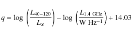
We also estimate $L_{\rm FIR}$ of each source using the available radio data and the well-known FIR-radio relation for local starbursts (Condon 1992). The original definition is based on the 60 $\mu$ m and 100 $\mu$ m flux densities, but following Sajina et al. (2008), we have adopted the definition:

$\begin{displaymath}q={\rm log}~\left(\frac{L_{40-120}}{L_{\odot}}\right)-{\rm log}~\left(\frac{L_{\rm 1.4~GHz}}{\rm W~Hz^{-1}}\right)+14.03 \end{displaymath}$

(4)

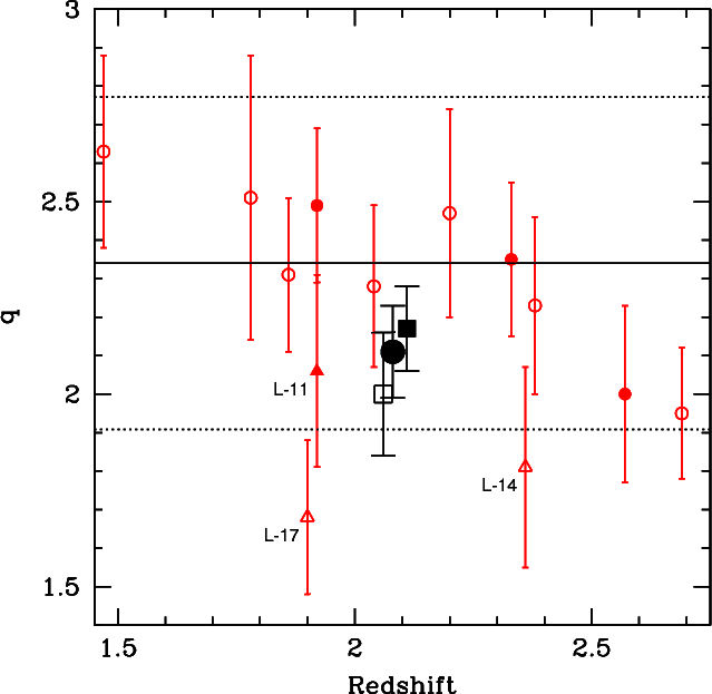
where L_40-120 is the integrated IR luminosity between 40 $\mu$ m and 120 $\mu$ m in the rest frame. We assume $L_{\rm FIR,mm} = L_{40-120}$ .

$\begin{figure} \par\resizebox{9cm}{!}{\includegraphics{12742f5.eps}}\end{figure}$

Figure 5:

The radio-FIR q factor (FIR-to-radio ratio) (Eq. (4)). The large black symbols show the stacked values of different samples: the entire sample (33 sources, filled circle), the 13 sources with S/N > 3 at 1.2 mm (filled square), and the 20 sources with S/N < 3 (open square). The solid black line shows the typical value q = 2.34 for local starbursts. The dotted black lines are the $3\sigma$ spread (Yun et al. 2001; Sajina et al. 2008). q values for individual sources are also shown for the sources with > $4\sigma$ detections at 1.2 mm (small filled symbols) and the sources with > $3\sigma$ signal (small open symbols). The red triangles show the sources identified as having the highest 20 cm/1.2 mm flux density ratios. The red circles are the sources with no 20 cm excess.

Open with DEXTER

Although Eq. (4) has been found to hold for local sources, its validity seems to be confirmed also at the redshifts of our sources (Kovács et al. 2006; Younger et al. 2009). The relation between $L_{\rm FIR}$ and the 20 cm or 50 cm flux density is thus straightforward, if we assume the typical value q = 2.34 and $L_{\rm FIR,mm} = L_{40-120}$

$\begin{displaymath}L_{\rm FIR}(L_{\odot})=2.04\times10^{-12}L_{\rm 1.4~GHz}({\rm W~Hz^{-1}}). \end{displaymath}$

(5)

However, this method is valid only if the radio emission is not significantly affected by an AGN. This expression will give an upper limit to the star-formation related $L_{\rm FIR}$ if an AGN contributes significantly to the radio emission. The $L_{\rm FIR}$ derived using Eq. (5), $L_{\rm {FIR,radio}}$ , are reported in Table 5.

The values of these two estimates of $L_{\rm FIR}$ are within a factor of 3 for most of the sample. They range from $\sim$ 0.5 to $\sim$ $10 \times 10^{12}~L_{\odot}$ , confirming that almost all our sources are ULIRGs with luminosities greater than $10^{12}~L_{\odot}$ . The average $L_{\rm FIR}$ derived from the radio flux densities is $\langle L_{\rm FIR,radio}\rangle = (4.14 \pm 0.53) \times 10^{12}~L_{\odot}$ . Since this value may be slightly overestimated because of AGN, it is consistent with $L_{\rm FIR}$ derived from fitting the median FIR SED, $\langle L_{\rm FIR} \rangle = 2.5 \times 10^{12}~L_{\odot}$ .

Alternatively, the radio-FIR relation (Eq. (5)) can be applied to identify or test for the presence of AGN-driven radio activity in our sample (similarly to Sect. 4.3 but slightly more rigorously). The agreement or deviation from this correlation can be easily expressed by the value of the q-factor, as reported in Table 5. We obtain an average value $\langle q\rangle =2.11\pm0.12$ for the whole sample.

This is not very different from the average value $\langle q \rangle = 2.34$ found for local star-forming galaxies (Yun et al. 2001). As shown in Fig. 5, the q-factors of the three sources identified as having the highest 20 cm/1.2 mm flux density ratios seem to be, on average, lower than those of most other sources. This is not surprising, since the q factor is another way to quantify the radio excess.

4.5 Stellar mass

The IRAC-based selection of our sample corresponds to a rest-frame NIR selection; therefore, if we ignore a possibly significant AGN contribution at these wavelengths, we are directly sampling the stellar component (Lo09). Applying the method developed by Berta et al. (2004), we have derived an estimation of the stellar mass for our sources. As summarized in Lo09, this derivation uses not only the IRAC data, but also optical and 24 $\mu$ m flux densities to perform a mixed stellar population spectro-photometric synthesis, and to constrain the extinction and the luminosity of young stellar populations (Berta et al. 2004). A redshift - here photometric - is also required. The stellar masses, initially computed with a 0.15-120 $M_{\odot }$ Salpeter (1955) initial mass function (IMF), are converted to a 0.10-100 $M_{\odot }$ IMF by applying a correction factor of 1.162 (Berta et al. 2003). All the stellar masses are shown in Table 5. Their values range from 0.8 to $7.2\times10^{11}$ $M_{\odot }$ , with a median value of $1.37\times10^{11}$ $M_{\odot }$ , and an average value $1.77\times 10^{11}$ $M_{\odot }$ .

As discussed in Lo09, these values may be somewhat overestimated for several reasons: our models may not fully take into account the TP-AGB contribution to infrared light (Maraston 2005); they assume a Salpeter-like IMF, which yields higher masses than other IMFs; and although the near-IR SED is dominated by stellar emission, it is possible that an AGN component is also present. Therefore, these estimates should be considered as upper limits to the true stellar masses, and may be overestimated by a small factor up to $\sim$ 2.

Using the same method, Lo09 found a median stellar mass $M_{\star}$ = $1.80\times10^{11}$ $M_{\odot }$ and an average value $2.16\times 10^{11}$ $M_{\odot }$ , about 30% larger than for our sample. This is consistent with the comparison of the average values of the 5.8 $\mu$ m flux density of both samples, which reflects the rest-frame luminosity at 1.6 $\mu$ m: 53 $\mu$ Jy for our sample and 77 $\mu$ Jy for that of Lo09. Indeed, as discussed by Lo09, the direct comparison of the NIR rest-frame luminosity at 1.6 $\mu$ m is probably the most consistent way to compare stellar masses in different samples, in order to avoid the dependence on the various methods applied to infer stellar masses from infrared fluxes. We have thus estimated the rest-frame luminosities at 1.6 $\mu$ m, $\nu L_{\nu}$ (1.6 $\mu$ m) (Table 5), by interpolating the observed IRAC fluxes as in Lo09. As expected, the average rest-frame luminosity at 1.6 $\mu$ m in Lo09, $4.1\times10^{11}$ $L_{\odot}$ , is a factor of 1.6 larger than for our sample, $2.5\times10^{11}$ $L_{\odot}$ (Table 5). The sources in our sample are as luminous as, or slightly more luminous at 1.6 $\mu$ m by a factor $\sim$ 1.5 than, submm selected SMGs, and should also be $\sim$ 1.5 times more massive than classical SMGs assuming the same mass-to-light ratio of Lo09. Our sample also shows a mass-to-light ratio consistent with the radio galaxy sample detected at 24 $\mu$ m by Seymour et al. (2007), who computed stellar masses directly from the luminosity at 1.6 $\mu$ m in the rest-frame.

4.6 Star formation rate

$\begin{figure} \par\includegraphics[width=8.8cm,clip]{12742f6.eps} \vspace*{-3mm} \end{figure}$

Figure 6:

(Adapted from Fig. 14 of Daddi et al. 2007). Star formation rate vs. stellar mass. Values of SFR deduced from radio data for the sources of our sample are represented by the red triangles (see Sects. 4.4, 4.6 and Table 5). The arrows are 2 $\sigma$ limits. The large black symbols show stacked values for different samples: all sources (radio determination = filled triangle, millimeter determination = open triangle), the sources with >3 $\sigma$ signal at 1.2 mm (radio determination = filled diamond, millimeter determination = open diamond), and the sources with <3 $\sigma$ signal at 1.2 mm (radio determination = filled circle, millimeter determination = open circle). The small black squares are for the 24 $\mu$ m BzK sources from GOODS (Daddi et al. 2007). The magenta star shows a typical value for SMGs. The large green squares trace the average SFR-mass relation in GOODS-N (160 arcmin²) determined from radio stacking of K < 20.5 galaxies in three mass bins; the blue line is SFR = 200 M₁₁^0.9 ( $M_{\odot }$ yr^-1), where M₁₁ is the stellar mass in units of 10¹¹ $M_{\odot }$ (Daddi et al. 2007).

Open with DEXTER

From the estimated $L_{\rm FIR}$ , we derive the star formation rate (SFR) of our sources assuming the relation from Kennicutt (1998) using a 0.10-100 $M_{\odot }$ Salpeter IMF:

$\begin{displaymath}{\it SFR}({\textit M}_{\odot}~{\rm yr}^{-1})\approx1.8\times10^{-10}{\textit L}_{\rm FIR}({\textit L}_{\odot}). \end{displaymath}$

(6)

The SFR values derived from $L_{\rm {FIR,mm}}$ and $L_{\rm {FIR,radio}}$ are listed in Table 5. The SFRs derived from $L_{\rm {FIR,radio}}$ for the sources with possible radio excess may be overestimated due to the possible AGN contribution to their radio emission. The mean SFR derived by averaging the radio-based estimates of all sources is $\sim$ 750 $M_{\odot }$ yr^-1; the mean derived from the average $L_{\rm FIR}$ is $\sim$ 450 $M_{\odot }$ yr^-1.

To estimate the contribution of ``5.8 $\mu$ m-peakers'' with $F_{\rm 24~\mu m}$ > 400 $\mu$ Jy to the star formation rate density (SFRD) of the universe, we consider the space density and average SFR of our sources. Assuming a redshift interval of 1.5<z<2.5, and an average SFR of 450 $M_{\odot }$ yr^-1, we derive the contribution of our sample to the (comoving) SFRD to be $\sim$ 1.5- $4\times 10^{-3}$ $M_{\odot }$ yr^-1 Mpc^-3. This value corresponds to $\sim$ 5% of the SFRD of all classical SMGs (Chapman et al. 2005; Aretxaga et al. 2007), i.e., to $\sim$ 10% of the SFRD of SMGs in the interval 1.5 <z< 2.5, and up to $\sim$ 15% in the interval of 1.7<z<2.3where ``5.8 $\mu$ m-peakers'' are mostly confined.

The specific star formation rate (SSFR), defined as SFR/ $M_{\star}$ , ranges from $\sim$ 10^-8 yr^-1 to $\sim$ 10^-9 yr^-1 for our sample. There is a tendency for the sources with the lowest stellar masses to have the highest SSFRs. This result is consistent with, e.g., Noeske et al. (2007). However, it is seen in Fig. 6 that ``5.8 $\mu$ m-peakers'' have significantly higher SSFRs than classical sBzK galaxies of comparable masses on average (Sect. 5.3).

5 Discussion

5.1 Comparison with other samples: 1) Spitzer selection (see Table 2)

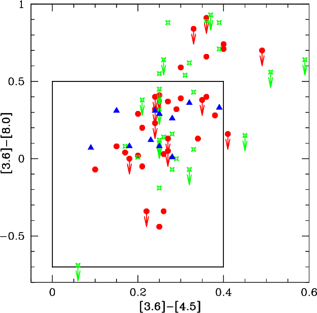
$\begin{figure} \par\resizebox{8.8cm}{!}{\includegraphics{12742f7.eps}} \end{figure}$

Figure 7:

IRAC color-color diagram for several samples. The sample of Huang et al. (2009) and Younger et al. (2009) is represented by the solid blue triangles. The red circles show our sample. The open green stars are the sample of Lonsdale et al. (2009). The arrows are 3 $\sigma$ upper limits for the difference [3.6]-[8.0]. The inset box shows the selection criteria of Huang et al. (2009). Magnitudes are on the AB scale.

Open with DEXTER

$\begin{figure} \par\resizebox{8.8cm}{!}{\includegraphics{12742f8.eps}} \end{figure}$

Figure 8:

Observed flux density ratio, $F_{\rm 1.2~mm}$ / $F_{\rm 24~\mu m}$ , versus redshift. The small filled (open) magenta circles are the $4\sigma$ detections (tentative $3\sigma$ detections) at 1.2 mm. The green arrows show the $2\sigma$ upper-limits for the other non-detections. The crosses show values for a sample of SMGs (see text). 1.2 mm flux densities for this sample were derived from $F_{\rm{850~\mu m}}$ when $F_{\rm 1.2~mm}$ is not available. The large symbols are the ratio of average flux density vs average redshift for different samples: all 33 of our sources (filled green square); all 13 of our sources with a > $3\sigma$ signal (magenta circle); the entire sample in Lo09 restricted to the Lockman Hole field (open blue triangle); the sources with signal > $3\sigma$ in Lo09 (filled blue triangle); the AGN-dominated 24 $\mu$ m bright sample of Lutz et al. (2005) (black pentagon); and the SMG literature sample (open star) (see Lo09, Ivison et al. 2007; Coppin et al. 2006). Expected values for various starburst and AGN templates are also shown (Lo09): starbursts Arp 220 (solid green line), M 82 (dot-dashed red line), and NGC 6090 (dotted magenta line); AGN-starburst composite IRAS19254-7245 South (dashed black line); and AGN ``QSO1'' (short-long-dashed blue line).

Open with DEXTER

The present work is an extension of the study presented in Lo09 on a sample of 61 sources selected in four SWIRE fields. The sources in Lo09 meet the same selection criteria and span the same redshift range, 1.4 $z_{\rm phot}$ 2.7, as our sample. However, their selection is biased toward brighter sources at 24 $\mu$ m, while the present sample is complete to a 24 $\mu$ m flux density limit of 400 $\mu$ Jy. This bias results in an average 24 $\mu$ m flux density a factor 1.5 greater than in our sample, $\langle F_{\rm {24~\mu m}}\rangle$ = 819 $\mu$ Jy vs. 566 $\mu$ Jy (see Sect. 2). Nevertheless, the 1.2 mm properties of the two samples are comparable. The average flux densities at 1.2 mm are similar: $1.56 \pm 0.22$ mJy for our entire sample, against $1.49 \pm 0.18$ mJy for the sample in Lo09.

Although the source selection in Lo09 was optimized to favor 1.2 mm bright sources, their detection rate is slightly lower than what we achieve with our complete sample, only 26% (31% in their best observed field with a sensitivity similar to ours) with ${\it S/N}>3$ $\sigma$ compared to 39% in our sample. Both samples are characterized by a similar average $L_{\rm FIR}$ determined using a thermal spectral model (see Sect. 4.4 and Eq. (3)), $\langle L_{\rm {FIR,mm}}\rangle$ = $2.5\pm 0.4\times10^{12}$ $L_{\odot}$ in this work vs. ( $2.8 \pm 0.1$ ) $\times$ 10¹² $L_{\odot}$ in Lo09 (restricted to the Lockman Hole field). Thus, in spite of the refinement implemented by Lo09 in their sample selection to increase the chance of finding mm bright sources among ``5.8 $\mu$ m peakers'', the average mm properties of their sample and our complete sample are consistent.

Younger et al. (2009) have studied the FIR properties of a similar Spitzer-selected sample, based on MIPS 70 and 160 $\mu$ m detections and MAMBO 1.2 mm observations. This sample (see also Huang et al. 2009) is selected based on IRAC colors, and 24 $\mu$ m flux densities (see Fig. 7, Table 2 and Sect. 2), yielding 12 starburst galaxies with overall properties (redshifts, IRAC colors, 1.2 mm flux densities) similar to those in Lo09 and in this work. Consequently, the $L_{\rm FIR}$ and derived star formation rates are also similar in all these samples.

Finally, Lutz et al. (2005) studied the mm properties of a Spitzer sample selected based on faint R band magnitudes, relatively bright 24 $\mu$ m flux densities ( $F_{\rm 24~\mu m}$ 1 mJy), and high $F_{\rm 24~\mu m}$ / $F_{\rm {8~\mu m}}$ ratios (Yan et al. 2007,2005; Sajina et al. 2008). This sample contains 40 sources at $z\sim 2$ exhibiting both starburst and AGN properties. They are on average fainter 1.2 mm emitters than our sources and they show significantly lower $F_{\rm 1.2~mm}$ / $F_{\rm 24~\mu m}$ flux density ratios, with $\langle F_{\rm {1.2~mm}}\rangle = 0.63 \pm 0.20$ mJy (simple average) and $\langle F_{\rm {1.2~mm}}\rangle/\langle F_{\rm {24~\mu m}}\rangle = 0.43$ (simple averages), compared to $\langle F_{\rm {1.2~mm}}\rangle =1.56 \pm 0.22$ mJy and $\langle F_{\rm {1.2~mm}}\rangle/\langle F_{\rm {24~\mu m}}\rangle =2.76\pm0.50$ for our sample (Table 3; see also Fig. 8). These differences are due to the fact that in the majority of these objects, the main source of power is an AGN rather than the powerful starburst required to produce bright mm flux, with the AGN dominating their 24 $\mu$ m emission.

5.2 Comparison with other samples: 2) Submillimetre selection

In order to characterize more quantitatively the difference in $F_{\rm 1.2~mm}$ / $F_{\rm 24~\mu m}$ flux density ratios between our sample of ``5.8 $\mu$ m-peakers'' and classical SMGs, we show them as a function of redshift in Fig. 8. The sample of classical SMGs is the sub-set of the sample used in Lo09 completed by the SHADES SMG sample from Coppin et al. (2006) and Ivison et al. (2007) detected at 24 $\mu$ m with 1.5 < z < 2.5. We also display a sub-set of ``5.8 $\mu$ m-peakers'' from Lo09. Note that most of the redshifts available for the Lo09 and the SHADES samples are photometric (Aretxaga et al. 2007). We also show in Fig. 8 the expected flux ratios for representative starburst and AGN templates. To facilitate the comparison, we also show the ratio of the average flux densities for the samples of ``5.8 $\mu$ m-peakers'' from this work and from Lo09, and for a sample of classical SMGs (the SMG sample of Lo09 augmented by those of SHADES: Ivison et al. 2007; Coppin et al. 2006). Our complete sample of ``5.8 $\mu$ m-peakers'' confirms that the ratio of the average 1.2 mm and 24 $\mu$ m flux densities for this class of sources is smaller than for SMGs. However, the difference is slightly smaller than in Lo09 because of our lower mean 24 $\mu$ m flux density. The $F_{\rm 1.2~mm}$ / $F_{\rm 24~\mu m}$ flux density ratios of our sample are also similar to one for the lensed LBG cB58, despite the fact that this lensed LBG is an order of magnitude less luminous than the average of our sample (Siana et al. 2008).

We have shown that ``5.8 $\mu$ m-peakers'' are $z\sim 2$ ULIRGs and that about 40% of them are bright mm sources. Thus, $\sim40\%$ of them also belong to the class of SMGs (Table 5), one of the main classes of high-z ULIRGs. A detailed comparison between the MIR and FIR properties of a large sample of SMGs (Hainline et al. 2009; Chapman et al. 2005; Borys et al. 2005; Frayer et al. 2004; Pope et al. 2005; Greve et al. 2004) and ``5.8 $\mu$ m-peakers'' is presented in Lo09. In this study, Lo09 find that most ``5.8 $\mu$ m-peakers'' represent a sub-class of SMGs. The differences found by Lo09 with respect to classical SMGs are mainly related to the selection criteria for the ``5.8 $\mu$ m-peakers''. More specifically, the Spitzer selection favours sources with redshifts mostly concentrated in the range $z~\sim 1.7$ -2.3, rather higher stellar masses than classical SMGs at similar redshifts, brighter 24 $\mu$ m flux densities, and thus higher $F_{\rm 1.2~mm}$ / $F_{\rm 24~\mu m}$ flux density ratios (see Fig. 9 in Lo09 and Fig. 8), and likely warmer dust temperatures. The mm-detected ``5.8 $\mu$ m-peakers'' and classical SMGs show similar mm/submm flux densities, implying that the main difference in the 1.2 mm/24 $\mu$ m ratio comes from the 24 $\mu$ m rather than the 1.2 mm intensity. This result implies that a high 24 $\mu$ m flux density does not directly translate into a high 1.2 mm flux density, and thus into high $L_{\rm FIR}$ and SFR, in starburst galaxies at $z\sim 2$ (see also Rieke et al. 2009; Pope et al. 2008a).

5.3 Nature of the sources: 1. Powerful starburst activity

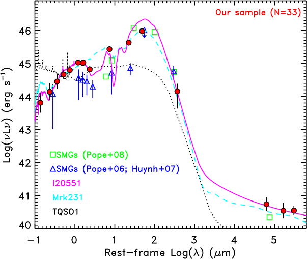
$\begin{figure} \par\resizebox{8.5cm}{!}{\includegraphics{12742f9.ps}} \end{figure}$

Figure 9:

Median optical through radio SED of all 33 ``5.8 $\mu$ m-peakers'' in our sample (red full circles). The 70 $\mu$ m and 160 $\mu$ m median values correspond to the stacked values of the central 21 sources (see Sect. 4.4). The magenta and cyan curves represent templates of IRAS 20551-4850 and Mrk 231 normalized to the rest-frame luminosity at 1.6 $\mu$ m. The black dotted curve represents a type 1 AGN template normalized at the lowest NIR data point (rest $\lambda$ = 2.4 $\mu$ m) of the median SED (Polletta et al. 2007). The blue triangles represent the average fluxes of the sample of 31 HDFN SMGs (Pope et al. 2006). The blue triangles at 70 $\mu$ m and 160 $\mu$ m correspond to the stacked fluxes for a subsample of 26 sources from the same sample (Huynh et al. 2007). The green open squares delineate the average SED of the GOODS SMGs derived by Pope et al. (2008b).

Open with DEXTER

As discussed in Sec. 2, our selection criteria are devised to distinguish starburst ULIRGs from AGN through the presence of the redshifted 1.6 $\mu$ m stellar ``bump'' which dominates over a strong AGN continuum in the near infrared. As shown by similar studies such as Weedman et al. (2006), Farrah et al. (2008), Huang et al. (2009), and Lo09, such criteria are very successful in selecting a majority of starbursts with strong mid-IR PAH features, and we have good evidence that this is also the case for the present sample from the combination of millimetre and radio data.

Although there might be some fraction of ``5.8 $\mu$ m-peakers'' that host a certain level of AGN activity, in the majority of these sources, the optical to far-IR light is likely dominated by starburst emission. This is confirmed by 1) the high detection rate at 1.2 mm and the high average value $\langle F_{\rm {1.2~mm}}\rangle$ = 1.56 mJy; and 2) the correlation between the mm and radio emission for the majority of the sources. With star formation rates ranging from a few 10² $M_{\odot }$ yr^-1to $\sim$ 10³ $M_{\odot }$ yr^-1 and a mean $\langle SFR \rangle$ $\gtrsim$ 450-750 $M_{\odot }$ yr^-1, they are powerful ULIRGs with starburst strengths similar to those of SMGs.

Significant emission in the mid-IR bands of PAHs is a common feature in starbursts (see, e.g., Desai et al. 2007; Rigopoulou et al. 1999; Farrah et al. 2009; Veilleux et al. 2009, for local galaxies). Although we are still lacking mid-IR spectroscopy for our $z\sim 2$ sample to infer the precise strength of the objects' PAH emission, there are very good reasons for thinking that it is strong and comparable to that observed in other 24 $\mu$ m-bright starburst galaxies at $z\sim 1.5{-}2$ satisfying similar criteria for selection of ``4.5 $\mu$ m-'' or ``5.8 $\mu$ m-peakers'' (Huang et al. 2009; Yan et al. 2007; Weedman et al. 2006; Murphy et al. 2009, Lonsdale et al. in prep.) or in about 30 ``4.5 $\mu$ m-peakers'' (Farrah et al. 2008). The strong PAH emission displayed in these objects accounts for the major part of the mid-IR emission in the range $\sim$ 6-12 $\mu$ m. It is thus clear that the PAHs generally contribute much of the flux detected in the Spitzer/MIPS broad 24 $\mu$ m band in such ``5.8 $\mu$ m-'' or ``4.5 $\mu$ m-peakers''. As noted, most SMGs have a much weaker 24 $\mu$ m intensity than our sources. It is not yet well understood why ``5.8 $\mu$ m-'' and ``4.5 $\mu$ m-peakers'' happen to have stronger PAH emission without a parallel enhancement of the observed mm/submm flux density, resulting in a higher 24 $\mu$ m/1.2 mm ratio than the bulk of the SMGs (Lo09). Farrah et al. (2008) suggest the possibility that star formation is extended on spatial scales of 1-4 kpc in such galaxies.

In Fig. 9, we show the median SED of our sample of ``5.8 $\mu$ m-peakers'', compared to the templates of a starburst, an obscured AGN, and an unobscured AGN. It is clear that the median observed SED is much better matched by the starburst template than by the obscured AGN SED, where the 5.8 $\mu$ m bump is absent.

$\begin{figure} \par\resizebox{8.5cm}{!}{\includegraphics{12742f10.eps}} \end{figure}$	Figure 10: BzK color-color plot for our sample. B magnitude is extrapolated from u and $g^{\prime }$ magnitudes. When z magnitude is missing, it is extrapoled from $i^{\prime }$ and J. Same symbols as Fig. 3. The black crosses are the sources with S/N < 3 at 1.2 mm. The solid black line shows the selection criterion for sBzKs of Daddi et al. (2004).
Open with DEXTER

``5.8 $\mu$ m-peakers'' (and ``4.5 $\mu$ m-peakers'') also have some relationship with other broader classes of infrared selected high-z star-forming galaxies, as judged by 24 $\mu$ m intensity. As already discussed (e.g., Table 3), there are various samples (e.g. Yan et al. 2005; Houck et al. 2005; Magliocchetti et al. 2007; Murphy et al. 2009) just selected as relatively strong at 24 $\mu$ m and weak in the optical, especially for the purpose of IRS mid-IR spectroscopy. One recent example is the so called ``Dust-Obscured Galaxies'' (DOGs) defined as having $S_{\rm {24~\mu m}}$ / $S_{\rm {R}}$ > 1000, with various limits for $S_{\rm {24~\mu m}}$ such as 300 $\mu$ Jy by Dey & The Ndwfs/MIPS Collaboration (2009); Dey et al. (2008), or 100 $\mu$ Jy by Pope et al. (2008a). However, such broad criteria select a mixture of starbursts and AGN, especially those with power-law IRAC SEDs. As seeing from Table 1, practically all sources of our sample satisfy or are close to the $S_{\rm {24~\mu m}}$ / $S_{\rm {R}}$ > 1000 flux density ratio defining DOGs.

A better established class of high-z galaxies partially selected from optical-NIR colors is the ``BzK'' galaxies (Daddi et al. 2004). This includes an ``sBzK'' sub-class of star-forming galaxies and a ``pBzK'' sub-class of passively evolving proto-ellipticals. Figure 10 shows that all sources in our sample with B, z, and K information are sBzK galaxies. ``5.8 $\mu$ m-peakers'' share the same redshift range as the bulk of BzKs (see e.g. Fig. 2 of Daddi et al. 2007). However, they are at the very top of the BzK luminosity function. This is clearly shown in Fig. 11 where we have put our sample of ``5.8 $\mu$ m-peakers'' on top of Fig. 7 of Daddi et al. (2007), which displays the rest luminosity $L_{\nu}$ (8 $\mu$ m) (roughly proportional to the bulk of $S_{\rm {24~\mu m}}$ ) and $L_{\rm {IR}}$ (deduced from $L_{\rm {1.4~GHz}}$ ) for all BzKs in the GOODS-N field.

We note that the two $z\sim 1.5$ BzKs where CO was recently detected by Daddi et al. (2008) are ``4.5 $\mu$ m-peakers'' with $S_{\rm {24~\mu m}}$ = 140 and 400 $\mu$ Jy and $L_{\rm {IR}}$ close to 10¹² $L_{\odot}$ , i.e., comparable to or below the lower end of the luminosity distribution of our sample (Fig. 11). This probably means that CO should be easily detectable in most of our ``5.8 $\mu$ m-peakers'' with the current sensitivity of the IRAM Plateau de Bure Interferometer (PdBI), as shown by Yan et al. (in prep.), who detected strong CO emission in two ``5.8 $\mu$ m-peakers'' of Sajina et al. (2008).

Since sBzK sources are major contributors to star formation at $z\sim 2$ , it is interesting to compare their star formation properties with those of our ``5.8 $\mu$ m-peakers''. Figure 6 shows that the average SFR of ``5.8 $\mu$ m-peakers'' is significantly greater than the average for sBzKs at $z\sim 2$ (Daddi et al. 2007). Even their SSFRs are significantly higher than those of sBzKs with comparable masses. This figure confirms that our ``5.8 $\mu$ m-peakers'' represent as significant a fraction of the most massive and star-forming sBzKs as Fig. 11 implies. On the other hand, as the average SFR of ``5.8 $\mu$ m-peakers'' is significantly lower than those of the bulk of classical SMGs, and their stellar mass slightly higher, it is not surprising that the mean SSFR of ``5.8 $\mu$ m-peakers'' is markedly smaller than one of SMGs (Fig. 6).

$\begin{figure} \par\includegraphics[width=8.5cm,clip]{12742f11.eps} \end{figure}$

Figure 11:

(Adapted from Fig. 7 of Daddi et al. 2007). Luminosity at 1.4 GHz rest frame vs. luminosity at 8 $\mu$ m rest frame. ``5.8 $\mu$ m-peakers'' from our sample are displayed as large red triangles. Data for all 24 $\mu$ m BzK sources of the GOODS-N field (Daddi et al. 2007) are shown for comparison as small black symbols; the three large green squares show the average trend vs. 8 $\mu$ m luminosity, including both radio-detected and radio-undetected sources from Daddi et al. (2007). The green stars are the two BzK sources with CO detections from Daddi et al. (2008).

Open with DEXTER

Another class of powerful starburst galaxies are the so called ``submillimetre faint radio galaxies'' (SFRGs; Chapman et al. 2008,2004; Blain et al. 2004). They are defined as radio sources with radio fluxes similar to those of SMGs which are not detected in typical SCUBA surveys. In addition to AGN, this class of sources may contain star-forming galaxies characterized by slightly hotter temperatures than typically observed in submillimetre galaxies. It is also possible that the radio properties and the hotter dust temperatures in these sources might be due to the presence of AGN activity, but clear evidence is still lacking for the relative fractions of AGN and hotter starbursts (Chapman et al. 2008; Casey et al. 2008,2009). It is thus interesting to consider whether our sources undetected at 1.2 mm and lying outside or at the outskirts of the radio-1.2 mm correlation might belong to the class of SFRG. More precisely, Chapman et al. (2008) propose to reserve the name of SFRG for radio sources with $L_{\rm {1.4~GHz}}$ > 10²⁴ W Hz^-1. As SFRGs must also not be detected in 850 $\mu$ m surveys with typical sensitivity 4 mJy, we assume that SFRGs in our sample may be defined by $L_{\rm {1.4~GHz}}$ > 10²⁴ W Hz^-1 and $F_{\rm 1.2~mm}$ < 1.6 mJy. SFRGs are identified with these criteria in Table 5. There are 3 confirmed SFRGs and 3 tentative SFRGs (together with 4 confirmed SMGs and 9 tentative SMGs defined as satisfying the limit $F_{\rm 1.2~mm}$ > 1.6 mJy, and 7 sources too weak in radio to be SFRG and at 1.2 mm to be SMG). We may thus estimate that among ``5.8 $\mu$ m-peakers'', at least $\sim$ 40% are SMGs, $\sim$ 10-20% may be SFRGs, and $\sim$ 15-20% are weak radio and mm sources.

5.4 Nature of the sources: 2. Weak AGN activity

Our selection criteria were designed to select starburst ULIRGs over AGN through the presence of the redshifted 1.6 $\mu$ m stellar ``bump''. However, similar studies have shown that the discrimination against AGN with such criteria is not perfect and that a small fraction has a weak but significant AGN contribution in their mid-IR SED. Since AGNs are powerful NIR emitters due to their ability to heat dust up to its sublimation temperature, we expect that such emission may smear out the 1.6 $\mu$ m stellar ``bump'', flatten it, or move to longer observed wavelengths (Daddi et al. 2007; Berta et al. 2007a). However, some AGNs can satisfy our selection criteria. Indeed, about 8 radio-galaxies from the sample of Seymour et al. (2007) follow our criteria. But these sources show a significant radio excess (Archibald et al. 2001; Reuland et al. 2004) due to the AGN.

To identify, quantify, and characterize any AGN activity which might be present in our sample it would be useful to have mid-IR spectroscopic data (see, e.g., Farrah et al. 2008; Weedman et al. 2006), optical/NIR spectroscopic data (Berta et al. 2007b; Chapman et al. 2005), morphological data from high angular resolution radio observations (see, e.g., Richards et al. 2007; Muxlow et al. 2005; Biggs & Ivison 2008), or deep X-ray data (see, e.g., Alexander et al. 2005). Only limited observations of this kind are available for our sample. A spectroscopic observation from Keck/LRIS is available for source L-25 (LH_574364 in Berta et al. 2007b). Based on one emission line identified as MgII, this source is classified as a type 2 AGN, although its radio/1.2 mm flux density ratio is not one of the highest and its radio spectral index instead point to a starburst-dominated IR SED (Table 4).

X-ray data of moderate depth (70 ks exposures) from Chandra are also available for all our sources (Polletta et al. 2006). None of them is detected by Chandra to a 0.3-8 keV flux limit of $3\times 10^{-15}$ erg cm^-2 s^-1. We stacked the X-ray images of all 33 sources, but no significant detection was obtained. We can only set an upper limit to the average 0.3-8 keV flux of 10^-16 erg cm^-2 s^-1 which corresponds to an average X-ray luminosity of 2 $\times$ 10⁴² erg s^-1. Such a low signal does not allow us to make any claim about the AGN contribution and X-ray properties of our sample.

The multi-frequency radio observations available for the majority of our sources may also allow us to investigate the AGN contribution. As discussed in Sect. 4.3, we can find some indication of AGN activity based on the 1.2 mm/radio flux density ratio complemented by the spectral index and the radio size; however, an extension may as easily reflect well an extended starburst as an AGN lobe.

Two 20 cm radio sources, L-17 and L-11, are specially strong ( $F_{\rm {20~cm}}> 300$ $\mu$ Jy). The 20 cm flux density of L-17 is slightly greater than 300 $\mu$ Jy, implying a 1.4 GHz luminosity close to 10²⁵ W Hz^-1 (see Fig. 12) which is close to the radio loudness limit at $z\sim 2$ (Jiang et al. 2007; Sajina et al. 2007). L-11, despite its high 20 cm flux, is not strictly radio loud according to this definition. Neither source is resolved in the radio; however, this might be not very meaningful, since both sources are in regions with limited sensitivity at 20 cm. Their spectral indices are -0.76 and -0.45, respectively, which is not very discriminating. Interestingly, both sources are rather strong and well detected at 1.2 mm (S/N = 3.5 and 5.3 respectively), implying that, if they are AGN, they might experience both starburst and accretion activity.

The two other sources with evidence of possible AGN-driven radio activity based on a high 20 cm/1.2 mm flux density ratio, L-8 and L-14, are not detected at 1.2 mm (S/N < 1 and S/N = 3, respectively), L-8 could be an SFRG, and L-14 either an SMG or an SFRG. L-8 is also extended in its radio image.

$\begin{figure} \par\resizebox{8.8cm}{!}{\includegraphics{12742f12.eps}} \end{figure}$	Figure 12: 1.4 GHz luminosity as function of redshift. Same symbols as Figs. 3 and 10. The solid black line shows the radio loudness limit for 1.4 GHz luminosity (Sajina et al. 2007).
Open with DEXTER

Table 6: Results from the co-added MIPS images.

6 Summary and conclusion

The aim of this project was to determine the average properties of a complete 24 $\mu$ m flux limited sample of bright Spitzer sources selected to be starburst dominated at $z\sim 2$ , using multi-wavelength data. The sample of 33 $z\sim 2$ SMG candidates was built with all the optically faint sources in a $\sim$ 0.5 deg² area of the Lockman Hole SWIRE field meeting selection criteria based on MIPS/IRAC fluxes. These criteria are $F_{\rm 24~\mu m}$ 400 mJy, a peak in the 5.8 $\mu$ m IRAC band due to redshifted 1.6 $\mu$ m stellar emission, and $r^\prime_{\rm Vega}$ > 23. The J1046+59 field was selected because of the availability of very deep radio observations at 20 cm and 90 cm with the VLA and at 50 cm with the GMRT. All sources in our sample are detected at 50 cm.

The entire sample has an average 1.2 mm flux density of 1.56 $\pm$ 0.22 mJy. However, the limited sensitivity allowed only four confirmed 4 $\sigma$ detections, plus nine tentative 3 $\sigma$ detections. Since the average 1.2 mm flux density, 1.56 mJy, corresponds to a 850 $\mu$ m flux density close to 4 mJy, about half of the sources may be considered SMGs. However, their redshifts range from $z\sim 1.7$ -2.3, similarly to the sample in Huang et al. (2009), but smaller than the redshift range covered by SMGs. The sample selected here is characterized by brighter 24 $\mu$ m flux densities, on average, than those of SMGs, and consequently shows systematically lower $F_{\rm 1.2~mm}$ / $F_{\rm 24~\mu m}$ ratios than classical SMGs. It is quite likely that our selection favours the SMGs with the brightest 24 $\mu$ m flux densities, due probably to enhanced PAH emission.

From stacking individual images of the sources, we are able to build the median FIR SED of our sample and estimate the corresponding $L_{\rm FIR}$ , SFR and $T_{\rm dust}$ assuming a single temperature ``greybody'' model. The inferred values are $T_{\rm dust}$ = 37 $\pm$ 8 K, $L_{\rm FIR}$ = 2.5 $\times$ 10¹² $L_{\odot}$ , and SFR = 450 $M_{\odot }$ yr^-1. These estimates indicate that most of the sources are ULIRGs. However, estimates of $L_{\rm FIR}$ for individual sources deduced from the IR-mm SED are highly uncertain due to the lack of flux measurements between 100 $\mu$ m and 500 $\mu$ m. The high quality radio data provide important complementary information on $L_{\rm FIR}$ and the star formation rate, since the 1.2 mm/radio flux density ratio of the majority of individual sources is consistent with the FIR/radio correlation, which allows a derivation of $L_{\rm FIR}$ and SFR from the radio flux, providing further confirmation that most of the selected sources are ULIRGs. The average value of $L_{\rm FIR}$ inferred from the FIR-radio correlation is $4.1\times 10^{12}$ $L_{\odot}$ ; however, this value may be overestimated because of an AGN contribution.

Stellar masses are estimated by modelling the optical-IR SED with stellar population synthesis models. They are of order a few 10¹¹ $M_{\odot }$ . Roughly scaling with the observed 5.8 $\mu$ m fluxes, they are similar to those of other samples of 24 $\mu$ m-bright, $z\sim 2$ Spitzer starbursts, and slightly higher than those of classical SMGs.

Overall, this sample appears similar to other samples of Spitzer $z\sim 2$ SMGs (Lo09; Younger et al. 2009) in terms of millimetre emission, $L_{\rm FIR}$ , and SFR.

The complete radio detection of all sources provides a good estimate of the total star formation rate of such sources. They represent a significant fraction of all SMGs in the redshift range $z\sim 1.7$ -2.3 ( $\sim$ 10-15%). Most of these ``5.8 $\mu$ m-peakers'' are star-forming BzK galaxies with luminosities at the top of the luminosity distribution of sBzKs.

The surface density of ``5.8 $\mu$ m-peakers'' has been found to be 61 deg^-2 by Farrah et al. (2006). This is consistent with 33 sources in the 0.49 deg² of our field. We may thus estimate that 40-60 similar ``5.8 $\mu$ m-peakers'' per square degree could be identified in the full SWIRE survey (49 deg²). Most of them should be $z\sim 2$ starburst ULIRGs. At least half of them may be considered to be SMGs, including a small fraction of composite obscured AGN/starburst objects. Another significant fraction may be considered as SFRGs.

These results illustrate the power of deep multi- $\lambda$ studies, especially with complete radio data, for analysing populations of powerful high-z IR and submm sources. Such deep radio data are essential for disentangling starbursts and infrared-bright AGN, and for easily providing estimates of their star formation rates. We note especially the impressive complete detection of relatively weak $z\sim 2$ SMGs over 0.5 deg² in a single pointing of the GMRT at 610 MHz. As already proved by the analysis of SCUBA sources (e.g., Ivison et al. 2002), radio data are essential for identifying optical/near-IR counterparts and analysing submm surveys. This will be even more crucial for future surveys at the confusion limits of instruments like Herschel at 300-500 $\mu$ m and SCUBA2 at 850 $\mu$ m. Even as we wait for EVLA and the new generation of SKA precursors, our results show that the GMRT at 610 MHz and even 325 MHz can already currently provide sensitivity well matched to wide Herschel surveys.

It would be interesting to explore further whether the main properties which characterize this sample, i.e. strong MIR emission, radio activity, and high stellar mass, are related. Some of these properties are likely the result of biases introduced by our selection; however, this is unlikely to be the case for all of them, especially for the radio properties. In particular, a comparison between the starburst morphology (traced by young stars, dust, PAHs or CO emission, as measured by ALMA or JWST) and the radio size would probe whether the radio emission is produced by the starburst or by an AGN, and whether the parameters of the starburst are different from those of most classical SMGs and reveal a different star formation regime.

We have several multi-wavelength observations planned or in progress for this sample to obtain better estimates of redshifts, dust temperatures, star formation rates, PAH luminosities, and AGN contributions, and thus constrain the dominant emission processes, and investigate the evolution and clustering properties of these sources.

Acknowledgements

We thank Roy Kilgard, Jacqueline Bergeron, Attila Kovács and Helmut Dannerbauer for their helpful contribution. This work includes observations made with IRAM, which is supported by INSU/CNRS (France), MPG (Germany) and IGN (Spain). Thanks to the staff of IRAM for their support and the anonymous observers of the MAMBO pool for observations presented here. This work is based in part on observations made within the context of SWIRE survey with the Spitzer Space Telescope, which is operated by the Jet Propulsion Laboratory, California Institute of Technology under a contract with NASA. The VLA is operated by NRAO, the National Radio Astronomy Observatory, a facility of the National Science Foundation operated under cooperative agreement by Associated Universities, Inc. We thank the staff of the GMRT who have made these observations possible. GMRT is run by the National Centre for Radio Astrophysics of the Tata Institute of Fundamental Research. The optical data come from KPNO (Kitt Peak National Observatory), National Optical Astronomy Observatory, which is operated by the Association of Universities for Research in Astronomy (AURA) under cooperative agreement with the National Science Foundation. This work includes observations made with WFCAM/UKIRT. The UKIRT is operated by the Joint Astronomy Centre on behalf of the UK's Science and Technology Facilities Council.

References

Alexander, D. M., Bauer, F. E., Chapman, S. C., et al. 2005, ApJ, 632, 736 [NASA ADS] [CrossRef]
Archibald, E. N., Dunlop, J. S., Hughes, D. H., et al. 2001, MNRAS, 323, 417 [NASA ADS] [CrossRef]
Aretxaga, I., Hughes, D. H., Coppin, K., et al. 2007, MNRAS, 379, 1571 [NASA ADS] [CrossRef]
Beelen, A., Cox, P., Benford, D. J., et al. 2006, ApJ, 642, 694 [NASA ADS] [CrossRef]
Berta, S., Fritz, J., Franceschini, A., Bressan, A., & Pernechele, C. 2003, A&A, 403, 119 [NASA ADS] [CrossRef] [EDP Sciences]
Berta, S., Fritz, J., Franceschini, A., Bressan, A., & Lonsdale, C. 2004, A&A, 418, 913 [NASA ADS] [CrossRef] [EDP Sciences]
Berta, S., Lonsdale, C. J., Polletta, M., et al. 2007a, A&A, 476, 151 [NASA ADS] [CrossRef] [EDP Sciences]
Berta, S., Lonsdale, C. J., Siana, B., et al. 2007b, A&A, 467, 565 [NASA ADS] [CrossRef] [EDP Sciences]
Biggs, A. D., & Ivison, R. J. 2008, MNRAS, 385, 893 [NASA ADS] [CrossRef]
Blain, A. W., Smail, I., Ivison, R. J., Kneib, J.-P., & Frayer, D. T. 2002, Phys. Rep., 369, 111 [NASA ADS] [CrossRef]
Blain, A. W., Chapman, S. C., Smail, I., & Ivison, R. 2004, ApJ, 611, 52 [NASA ADS] [CrossRef]
Bolzonella, M., Miralles, J.-M., & Pelló, R. 2000, A&A, 363, 476 [NASA ADS]
Borys, C., Smail, I., Chapman, S. C., et al. 2005, ApJ, 635, 853 [NASA ADS] [CrossRef]
Casey, C. M., Impey, C. D., Trump, J. R., et al. 2008, ApJS, 177, 131 [NASA ADS] [CrossRef]
Casey, C. M., Chapman, S. C., Beswick, R. J., et al. 2009, MNRAS, 1097
Chapman, S. C., Smail, I., Windhorst, R., Muxlow, T., & Ivison, R. J. 2004, ApJ, 611, 732 [NASA ADS] [CrossRef]
Chapman, S. C., Blain, A. W., Smail, I., & Ivison, R. J. 2005, ApJ, 622, 772 [NASA ADS] [CrossRef]
Chapman, S. C., Neri, R., Bertoldi, F., et al. 2008, ApJ, 689, 889 [NASA ADS] [CrossRef]
Ciliegi, P., Vignali, C., Comastri, A., et al. 2003, MNRAS, 342, 575 [NASA ADS] [CrossRef]
Condon, J. J. 1992, ARA&A, 30, 575 [NASA ADS] [CrossRef]
Coppin, K., Chapin, E. L., Mortier, A. M. J., et al. 2006, MNRAS, 372, 1621 [NASA ADS] [CrossRef]
Crawford, T., Marr, J., Partridge, B., & Strauss, M. A. 1996, ApJ, 460, 225 [NASA ADS] [CrossRef]
Daddi, E., Cimatti, A., Renzini, A., et al. 2004, ApJ, 617, 746 [NASA ADS] [CrossRef]
Daddi, E., Dickinson, M., Morrison, G., et al. 2007, ApJ, 670, 156 [NASA ADS] [CrossRef]
Daddi, E., Dannerbauer, H., Elbaz, D., et al. 2008, ApJ, 673, L21 [NASA ADS] [CrossRef]
De Breuck, C., van Breugel, W., Röttgering, H. J. A., & Miley, G. 2000, A&AS, 143, 303 [NASA ADS] [CrossRef] [EDP Sciences]
De Breuck, C., van Breugel, W., Röttgering, H., et al. 2001, AJ, 121, 1241 [NASA ADS] [CrossRef]
Desai, V., Armus, L., Spoon, H. W. W., et al. 2007, ApJ, 669, 810 [NASA ADS] [CrossRef]
Dey, A., Soifer, B. T., Desai, V., et al. 2008, ApJ, 677, 943 [NASA ADS] [CrossRef]
Dey, A., & The Ndwfs/MIPS Collaboration 2009, ed. W. Wang, Z. Yang, Z. Luo, & Z. Chen, ASP Conf. Ser., 408, 411
Downes, A. J. B., Peacock, J. A., Savage, A., & Carrie, D. R. 1986, MNRAS, 218, 31 [NASA ADS]
Dye, S., Eales, S. A., Aretxaga, I., et al. 2008, MNRAS, 386, 1107 [NASA ADS] [CrossRef]
Farrah, D., Lonsdale, C. J., Borys, C., et al. 2006, ApJ, 641, L17 [NASA ADS] [CrossRef]
Farrah, D., Lonsdale, C. J., Weedman, D. W., et al. 2008, ApJ, 677, 957 [NASA ADS] [CrossRef]
Farrah, D., Connolly, B., Connolly, N., et al. 2009, ApJ, 700, 395 [NASA ADS] [CrossRef]
Frayer, D. T., Chapman, S. C., Yan, L., et al. 2004, ApJS, 154, 137 [NASA ADS] [CrossRef]
Greve, T. R., Ivison, R. J., Bertoldi, F., et al. 2004, MNRAS, 354, 779 [NASA ADS] [CrossRef]
Hainline, L. J., Blain, A. W., Smail, I., et al. 2009, ApJ, 699, 1610 [NASA ADS] [CrossRef]
Hambly, N. C., Collins, R. S., Cross, N. J. G., et al. 2008, MNRAS, 384, 637 [NASA ADS] [CrossRef]
Helou, G., Soifer, B. T., & Rowan-Robinson, M. 1985, ApJ, 298, L7 [NASA ADS] [CrossRef]
Henry, D. M., Atad-Ettedgui, E., Casali, M. M., et al. 2000, in SPIE Conf. Ser., ed. M. Iye, & A. F. Moorwood, 4008, 1325
Holland, W. S., Robson, E. I., Gear, W. K., et al. 1999, MNRAS, 303, 659 [NASA ADS] [CrossRef]
Houck, J. R., Soifer, B. T., Weedman, D., et al. 2005, ApJ, 622, L105 [NASA ADS] [CrossRef]
Huang, J., Faber, S. M., Daddi, E., et al. 2009, ApJ, 700, 183 [NASA ADS] [CrossRef]
Huynh, M. T., Pope, A., Frayer, D. T., & Scott, D. 2007, ApJ, 659, 305 [NASA ADS] [CrossRef]
Ibar, E., Cirasuolo, M., Ivison, R., et al. 2008, MNRAS, 386, 953 [NASA ADS] [CrossRef]
Ivison, R. J., Greve, T. R., Smail, I., et al. 2002, MNRAS, 337, 1 [NASA ADS] [CrossRef]
Ivison, R. J., Greve, T. R., Dunlop, J. S., et al. 2007, MNRAS, 380, 199 [NASA ADS] [CrossRef]
Jiang, L., Fan, X., Ivezic, Z., et al. 2007, ApJ, 656, 680 [NASA ADS] [CrossRef]
Kennicutt, Jr., R. C. 1998, ARA&A, 36, 189 [NASA ADS] [CrossRef]
Kovács, A., Chapman, S. C., Dowell, C. D., et al. 2006, ApJ, 650, 592 [NASA ADS] [CrossRef]
Kreysa, E., Gemuend, H.-P., Gromke, J., et al. 1998, in Advanced Technology MMW, Radio, and Terahertz Telescopes, Presented at the SPIE Conf. Ser., ed. T. G. Phillips, Proc. SPIE, 3357, 319
Lawrence, A., Warren, S. J., Almaini, O., et al. 2007, MNRAS, 379, 1599 [NASA ADS] [CrossRef]
Le Floc'h, E., Papovich, C., Dole, H., et al. 2005, ApJ, 632, 169 [NASA ADS] [CrossRef]
Lonsdale, C. J., Smith, H. E., Rowan-Robinson, M., et al. 2003, PASP, 115, 897 [NASA ADS] [CrossRef]
Lonsdale, C. J., Omont, A., Polletta, M. D. C., et al. 2006, BAAS, 38, 1171 [NASA ADS]
Lonsdale, C. J., Polletta, M. D. C., Omont, A., et al. 2009, ApJ, 692, 422 [NASA ADS] [CrossRef] [Lo09]
Lutz, D., Yan, L., Armus, L., et al. 2005, ApJ, 632, L13 [NASA ADS] [CrossRef]
Magliocchetti, M., Silva, L., Lapi, A., et al. 2007, MNRAS, 375, 1121 [NASA ADS] [CrossRef]
Maraston, C. 2005, MNRAS, 362, 799 [NASA ADS] [CrossRef]
Muller, G. P., Reed, R., Armandroff, T., Boroson, T. A., & Jacoby, G. H. 1998, in SPIE Conf. Ser., 3355, 577
Murphy, E. J., Chary, R.-R., Alexander, D. M., et al. 2009, ApJ, 698, 1380 [NASA ADS] [CrossRef]
Murphy, Jr., T. W., Soifer, B. T., Matthews, K., & Armus, L. 2001, ApJ, 559, 201 [NASA ADS] [CrossRef]
Muxlow, T. W. B., Richards, A. M. S., Garrington, S. T., et al. 2005, MNRAS, 358, 1159 [NASA ADS] [CrossRef]
Noeske, K. G., Faber, S. M., Weiner, B. J., et al. 2007, ApJ, 660, L47 [NASA ADS] [CrossRef]
Owen, F. N., & Morrison, G. E. 2008, AJ, 136, 1889 [NASA ADS] [CrossRef]
Owen, F. N., Morrison, G. E., Klimek, M. D., & Greisen, E. W. 2009, AJ, 137
Polletta, M., Courvoisier, T. J.-L., Hooper, E. J., & Wilkes, B. J. 2000, A&A, 362, 75 [NASA ADS]
Polletta, M., Wilkes, B. J., Siana, B., et al. 2006, ApJ, 642, 673 [NASA ADS] [CrossRef]
Polletta, M., Tajer, M., Maraschi, L., et al. 2007, ApJ, 663, 81 [NASA ADS] [CrossRef]
Pope, A., Borys, C., Scott, D., et al. 2005, MNRAS, 358, 149 [NASA ADS] [CrossRef]
Pope, A., Scott, D., Dickinson, M., et al. 2006, MNRAS, 370, 1185 [NASA ADS] [CrossRef]
Pope, A., Bussmann, R. S., Dey, A., et al. 2008a, ApJ, 689, 127 [NASA ADS] [CrossRef]
Pope, A., Chary, R.-R., Alexander, D. M., et al. 2008b, ApJ, 675, 1171 [NASA ADS] [CrossRef]
Reuland, M., Röttgering, H., van Breugel, W., & De Breuck, C. 2004, MNRAS, 353, 377 [NASA ADS] [CrossRef]
Richards, A. M. S., Muxlow, T. W. B., Beswick, R., et al. 2007, A&A, 472, 805 [NASA ADS] [CrossRef] [EDP Sciences]
Rieke, G. H., Alonso-Herrero, A., Weiner, B. J., et al. 2009, ApJ, 692, 556 [NASA ADS] [CrossRef]
Rigopoulou, D., Spoon, H. W. W., Genzel, R., et al. 1999, AJ, 118, 2625 [NASA ADS] [CrossRef]
Rowan-Robinson, M., Babbedge, T., Oliver, S., et al. 2008, MNRAS, 386, 697 [NASA ADS] [CrossRef]
Sajina, A., Yan, L., Armus, L., et al. 2007, ApJ, 664, 713 [NASA ADS] [CrossRef]
Sajina, A., Yan, L., Lutz, D., et al. 2008, ApJ, 683, 659 [NASA ADS] [CrossRef]
Salpeter, E. E. 1955, ApJ, 121, 161 [NASA ADS] [CrossRef]
Sanders, D. B., & Mirabel, I. F. 1996, ARA&A, 34, 749 [NASA ADS] [CrossRef]
Seymour, N., Stern, D., De Breuck, C., et al. 2007, ApJS, 171, 353 [NASA ADS] [CrossRef]
Seymour, N., Dwelly, T., Moss, D., et al. 2008, MNRAS, 386, 1695 [NASA ADS] [CrossRef]
Siana, B., Teplitz, H. I., Chary, R.-R., Colbert, J., & Frayer, D. T. 2008, ApJ, 689, 59 [NASA ADS] [CrossRef]
Siringo, G., Kreysa, E., Kovács, A., et al. 2009, A&A, 497, 945 [NASA ADS] [CrossRef] [EDP Sciences]
Smail, I., Ivison, R. J., Blain, A. W., & Kneib, J.-P. 2002, MNRAS, 331, 495 [NASA ADS] [CrossRef]
Solomon, P. M., & Vanden Bout, P. A. 2005, ARA&A, 43, 677 [NASA ADS] [CrossRef]
Spergel, D. N., Verde, L., Peiris, H. V., et al. 2003, ApJS, 148, 175 [NASA ADS] [CrossRef]
Surace, J. A., Shupe, D. L., Fang, F., et al. 2005, Data Delivery Document (Spitzer Science Center, California Institute of Technology, Pasadena, CA)
Veilleux, S., Rupke, D. S. N., Kim, D.-C., et al. 2009, ApJS, 182, 628 [NASA ADS] [CrossRef]
Warren, S. J., Hambly, N. C., Dye, S., et al. 2007, MNRAS, 375, 213 [NASA ADS] [CrossRef]
Weedman, D., Polletta, M., Lonsdale, C. J., et al. 2006, ApJ, 653, 101 [NASA ADS] [CrossRef]
Wilson, J. C., Eikenberry, S. S., Henderson, C. P., et al. 2003, in SPIE Conf. Ser., ed. M. Iye, & A. F. M. Moorwood, 4841, 451
Yan, L., Chary, R., Armus, L., et al. 2005, ApJ, 628, 604 [NASA ADS] [CrossRef]
Yan, L., Sajina, A., Fadda, D., et al. 2007, ApJ, 658, 778 [NASA ADS] [CrossRef]
Younger, J. D., Omont, A., Fiolet, N., et al. 2009, MNRAS, 394, 1685 [NASA ADS] [CrossRef]
Yun, M. S., & Carilli, C. L. 2002, ApJ, 568, 88 [NASA ADS] [CrossRef]
Yun, M. S., Reddy, N. A., & Condon, J. J. 2001, ApJ, 554, 803 [NASA ADS] [CrossRef]

Online Material

Appendix A: SED fits and photometric redshifts

The optical (Ugriz), NIR (JHK), and MIR (3.6-24 $\mu$ m) SEDs of each source have been fitted with a library of 18 star-forming galaxy templates (Polletta et al. 2007) using the H YPER-Z code (Bolzonella et al. 2000) and the same procedure described in Lonsdale et al. (2009). In Fig. A.1, we show the optical-IR SED and the best-fit template and corresponding photometric redshift of each source. In seven cases we also report a secondary solution corresponding to a second minimum in the $\chi ^2$ distribution if associated with a different template than the primary solution. In case a spectroscopic redshift is available (source L-25), the best-fit template at the spectroscopic redshift is also reported.

$\begin{figure} \par\includegraphics{12742ap1.ps} \end{figure}$

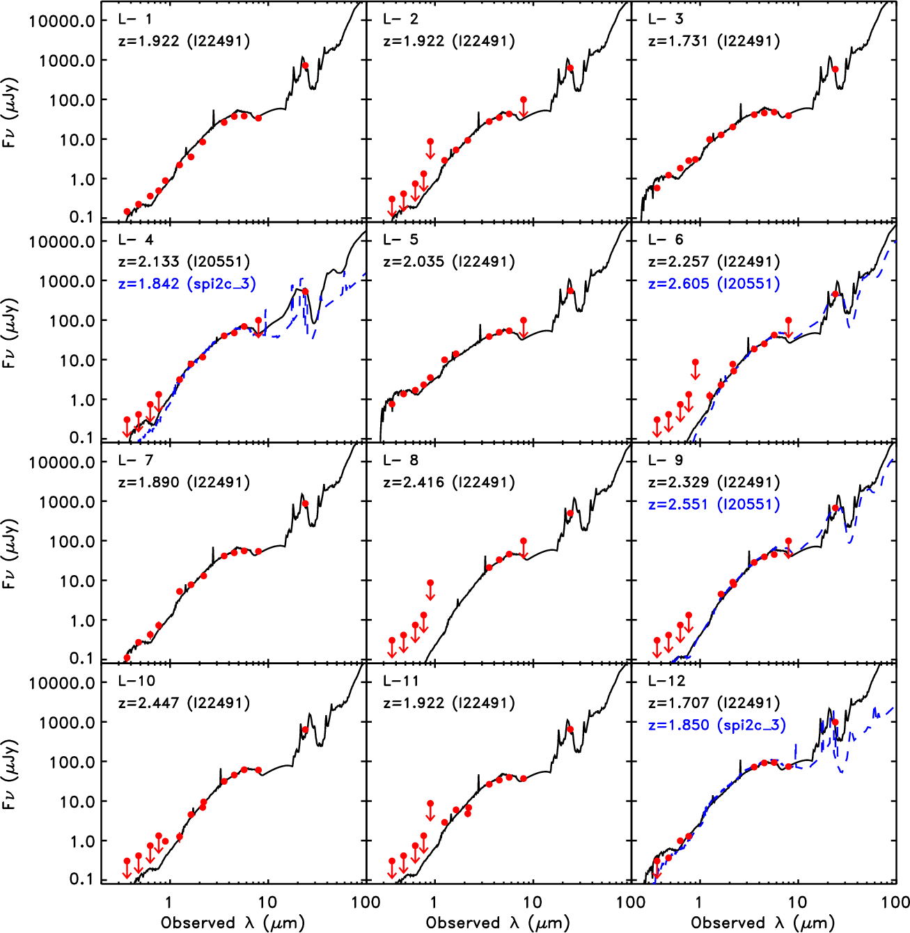
Figure A.1:

Optical-IR SEDs of our sources. The solid curves represent the best-fit template of the optical-MIR data (up to 24 $\mu$ m). The dashed blue curves correspond to fits with increasing $\chi ^2$ . The template name and photometric redshifts of each fit are annotated. For L-25, the dotted curve corresponds to the best-fit template plotted at the spectroscopic redshift. The source ID number is reported in each panel. Downward arrows represent 5 $\sigma$ upper limits at optical and infrared wavelengths.

Open with DEXTER

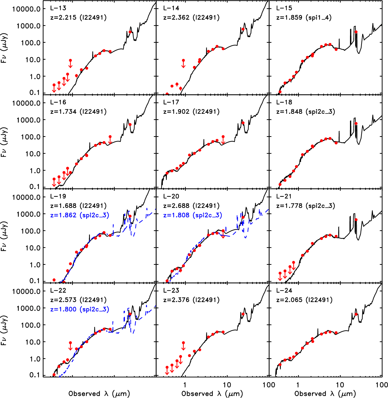
$\begin{figure} \includegraphics{12742ap2.ps} \end{figure}$	Figure A.1: continued.
Open with DEXTER

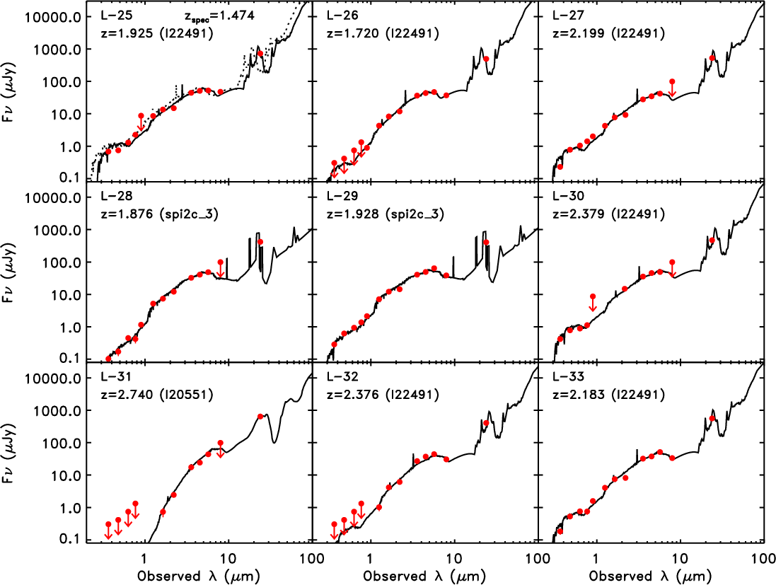
$\begin{figure} \includegraphics{12742ap3.ps} \end{figure}$	Figure A.1: continued.
Open with DEXTER

Footnotes

...z $\sim$ 2: Color figures and the Appendix A are only available in the electronic form via http://www.aanda.org
... package: Documentation by Zylka is available at http://www.iram.es/IRAMES/mainWiki/CookbookMopsic
... CA): http://swire.irac.caltech.edu/swire/astronomers/publications/SWIRE2_doc_083105.pdf

All Tables

Table 1: Optical, Near-IR and Spitzer mid-IR data of the selected sample.

Table 2: Related Spitzer-selected $z\sim 2$ ULIRGs samples.

Table 3: Derived values from the stacked flux densities^a.

Table 4: 1.2 mm and radio data.

Table 5: Luminosities and star formation rates.

Table 6: Results from the co-added MIPS images.

All Figures

$\begin{figure} \par\resizebox{8.5cm}{!}{\includegraphics{12742f1.eps}} \end{figure}$	Figure 1: Positions of the 33 sources of our sample ( $42^\prime \times 42^\prime$ J1046+59 field, centred at the VLA position observed by Owen & Morrison (2008), $\alpha _{2000}=10$ h46m00s, $\delta_{2000}=+59\degr01\hbox{$^\prime$ }00\hbox{$^{\prime\prime}$ }$ ). The red filled triangles are the $4\sigma$ detections at 1.2 mm. The green filled circles are the $3\sigma$ tentative detections at 1.2 mm. The blue squares are sources with a signal at 1.2 mm lower than $3\sigma$ . The sizes of symbols are proportional to 1.2 mm strengths. The open symbols show no detection at 20 cm (Owen & Morrison 2008).
Open with DEXTER
In the text

$\begin{figure} \par\resizebox{8.8cm}{!}{\includegraphics{12742f2.eps}} \end{figure}$	Figure 2: Histogram of redshifts for our sample (photometric, thick solid red line), the full sample from Lo09 (photometric and spectroscopic, dotted black line), and the sample from Younger et al. (2009) (spectroscopic, long-short-dashed blue line).
Open with DEXTER
In the text

$\begin{figure} \par\resizebox{8.8cm}{!}{\includegraphics{12742f3.eps}} \end{figure}$	Figure 3: Observed MAMBO 1.2 mm flux density as a function of 24 $\mu$ m flux density. The black squares show the average flux densities for the first $F_{\rm 24~\mu m}$ quartile (8 sources) and for the 25 other sources, respectively. The filled (open) red circles are the sources that are $4\sigma$ detections ( $3\sigma$ tentative detections) at 1.2 mm. The green arrows are 2 $\sigma$ upper limits for the sources that are not detected at 1.2 mm.
Open with DEXTER
In the text

$\begin{figure} \par\resizebox{8.8cm}{!}{\includegraphics{12742f4.eps}} \end{figure}$	Figure 4: Observed MAMBO 1.2 mm flux density as a function of 20 cm flux density. The large black symbols show different stacked values: the entire sample (filled triangle), all sources with > $3\sigma$ (filled diamond), the sources with > $3\sigma$ signal without the two strongest radio sources (open square), and the sources with <3 $\sigma$ signal (filled square). The filled (open) red circles are the sources that are $4\sigma$ detections ( $3\sigma$ tentative detections) at 1.2 mm. The green arrows are 2 $\sigma$ upper limits for the sources with S/N < 3 at 1.2 mm. The solid black line shows the correlation derived from Chapman et al. (2005) for $z\simeq 2$ (assuming $F_{\rm 850~\mu m}/F_{\rm 1.2~mm} = 2.5$ at $z\sim 2$ ). The dashed lines are the limits of this correlation at $\pm$ $1\sigma$ . The labelled sources are those with the highest 20 cm/1.2 mm flux density ratios (see Table 4).
Open with DEXTER
In the text

$\begin{figure} \par\resizebox{9cm}{!}{\includegraphics{12742f5.eps}}\end{figure}$	Figure 5: The radio-FIR q factor (FIR-to-radio ratio) (Eq. (4)). The large black symbols show the stacked values of different samples: the entire sample (33 sources, filled circle), the 13 sources with S/N > 3 at 1.2 mm (filled square), and the 20 sources with S/N < 3 (open square). The solid black line shows the typical value q = 2.34 for local starbursts. The dotted black lines are the $3\sigma$ spread (Yun et al. 2001; Sajina et al. 2008). q values for individual sources are also shown for the sources with > $4\sigma$ detections at 1.2 mm (small filled symbols) and the sources with > $3\sigma$ signal (small open symbols). The red triangles show the sources identified as having the highest 20 cm/1.2 mm flux density ratios. The red circles are the sources with no 20 cm excess.
Open with DEXTER
In the text

$\begin{figure} \par\includegraphics[width=8.8cm,clip]{12742f6.eps} \vspace*{-3mm} \end{figure}$	Figure 6: (Adapted from Fig. 14 of Daddi et al. 2007). Star formation rate vs. stellar mass. Values of SFR deduced from radio data for the sources of our sample are represented by the red triangles (see Sects. 4.4, 4.6 and Table 5). The arrows are 2 $\sigma$ limits. The large black symbols show stacked values for different samples: all sources (radio determination = filled triangle, millimeter determination = open triangle), the sources with >3 $\sigma$ signal at 1.2 mm (radio determination = filled diamond, millimeter determination = open diamond), and the sources with <3 $\sigma$ signal at 1.2 mm (radio determination = filled circle, millimeter determination = open circle). The small black squares are for the 24 $\mu$ m BzK sources from GOODS (Daddi et al. 2007). The magenta star shows a typical value for SMGs. The large green squares trace the average SFR-mass relation in GOODS-N (160 arcmin²) determined from radio stacking of K < 20.5 galaxies in three mass bins; the blue line is SFR = 200 M₁₁^0.9 ( $M_{\odot }$ yr^-1), where M₁₁ is the stellar mass in units of 10¹¹ $M_{\odot }$ (Daddi et al. 2007).
Open with DEXTER
In the text

$\begin{figure} \par\resizebox{8.8cm}{!}{\includegraphics{12742f7.eps}} \end{figure}$	Figure 7: IRAC color-color diagram for several samples. The sample of Huang et al. (2009) and Younger et al. (2009) is represented by the solid blue triangles. The red circles show our sample. The open green stars are the sample of Lonsdale et al. (2009). The arrows are 3 $\sigma$ upper limits for the difference [3.6]-[8.0]. The inset box shows the selection criteria of Huang et al. (2009). Magnitudes are on the AB scale.
Open with DEXTER
In the text

$\begin{figure} \par\resizebox{8.8cm}{!}{\includegraphics{12742f8.eps}} \end{figure}$	Figure 8: Observed flux density ratio, $F_{\rm 1.2~mm}$ / $F_{\rm 24~\mu m}$ , versus redshift. The small filled (open) magenta circles are the $4\sigma$ detections (tentative $3\sigma$ detections) at 1.2 mm. The green arrows show the $2\sigma$ upper-limits for the other non-detections. The crosses show values for a sample of SMGs (see text). 1.2 mm flux densities for this sample were derived from $F_{\rm{850~\mu m}}$ when $F_{\rm 1.2~mm}$ is not available. The large symbols are the ratio of average flux density vs average redshift for different samples: all 33 of our sources (filled green square); all 13 of our sources with a > $3\sigma$ signal (magenta circle); the entire sample in Lo09 restricted to the Lockman Hole field (open blue triangle); the sources with signal > $3\sigma$ in Lo09 (filled blue triangle); the AGN-dominated 24 $\mu$ m bright sample of Lutz et al. (2005) (black pentagon); and the SMG literature sample (open star) (see Lo09, Ivison et al. 2007; Coppin et al. 2006). Expected values for various starburst and AGN templates are also shown (Lo09): starbursts Arp 220 (solid green line), M 82 (dot-dashed red line), and NGC 6090 (dotted magenta line); AGN-starburst composite IRAS19254-7245 South (dashed black line); and AGN ``QSO1'' (short-long-dashed blue line).
Open with DEXTER
In the text

$\begin{figure} \par\resizebox{8.5cm}{!}{\includegraphics{12742f9.ps}} \end{figure}$	Figure 9: Median optical through radio SED of all 33 ``5.8 $\mu$ m-peakers'' in our sample (red full circles). The 70 $\mu$ m and 160 $\mu$ m median values correspond to the stacked values of the central 21 sources (see Sect. 4.4). The magenta and cyan curves represent templates of IRAS 20551-4850 and Mrk 231 normalized to the rest-frame luminosity at 1.6 $\mu$ m. The black dotted curve represents a type 1 AGN template normalized at the lowest NIR data point (rest $\lambda$ = 2.4 $\mu$ m) of the median SED (Polletta et al. 2007). The blue triangles represent the average fluxes of the sample of 31 HDFN SMGs (Pope et al. 2006). The blue triangles at 70 $\mu$ m and 160 $\mu$ m correspond to the stacked fluxes for a subsample of 26 sources from the same sample (Huynh et al. 2007). The green open squares delineate the average SED of the GOODS SMGs derived by Pope et al. (2008b).
Open with DEXTER
In the text

$\begin{figure} \par\resizebox{8.5cm}{!}{\includegraphics{12742f10.eps}} \end{figure}$	Figure 10: BzK color-color plot for our sample. B magnitude is extrapolated from u and $g^{\prime }$ magnitudes. When z magnitude is missing, it is extrapoled from $i^{\prime }$ and J. Same symbols as Fig. 3. The black crosses are the sources with S/N < 3 at 1.2 mm. The solid black line shows the selection criterion for sBzKs of Daddi et al. (2004).
Open with DEXTER
In the text

$\begin{figure} \par\includegraphics[width=8.5cm,clip]{12742f11.eps} \end{figure}$	Figure 11: (Adapted from Fig. 7 of Daddi et al. 2007). Luminosity at 1.4 GHz rest frame vs. luminosity at 8 $\mu$ m rest frame. ``5.8 $\mu$ m-peakers'' from our sample are displayed as large red triangles. Data for all 24 $\mu$ m BzK sources of the GOODS-N field (Daddi et al. 2007) are shown for comparison as small black symbols; the three large green squares show the average trend vs. 8 $\mu$ m luminosity, including both radio-detected and radio-undetected sources from Daddi et al. (2007). The green stars are the two BzK sources with CO detections from Daddi et al. (2008).
Open with DEXTER
In the text

$\begin{figure} \par\resizebox{8.8cm}{!}{\includegraphics{12742f12.eps}} \end{figure}$	Figure 12: 1.4 GHz luminosity as function of redshift. Same symbols as Figs. 3 and 10. The solid black line shows the radio loudness limit for 1.4 GHz luminosity (Sajina et al. 2007).
Open with DEXTER
In the text

$\begin{figure} \par\includegraphics{12742ap1.ps} \end{figure}$	Figure A.1: Optical-IR SEDs of our sources. The solid curves represent the best-fit template of the optical-MIR data (up to 24 $\mu$ m). The dashed blue curves correspond to fits with increasing $\chi ^2$ . The template name and photometric redshifts of each fit are annotated. For L-25, the dotted curve corresponds to the best-fit template plotted at the spectroscopic redshift. The source ID number is reported in each panel. Downward arrows represent 5 $\sigma$ upper limits at optical and infrared wavelengths.
Open with DEXTER
In the text

$\begin{figure} \includegraphics{12742ap2.ps} \end{figure}$	Figure A.1: continued.
Open with DEXTER
In the text

$\begin{figure} \includegraphics{12742ap3.ps} \end{figure}$	Figure A.1: continued.
Open with DEXTER
In the text

Current usage metrics show cumulative count of Article Views (full-text article views including HTML views, PDF and ePub downloads, according to the available data) and Abstracts Views on Vision4Press platform.

Data correspond to usage on the plateform after 2015. The current usage metrics is available 48-96 hours after online publication and is updated daily on week days.

Initial download of the metrics may take a while.