


| Issue |
A&A
Volume 712, August 2026
|
|
|---|---|---|
| Article Number | A58 | |
| Number of page(s) | 16 | |
| Section | Planets, planetary systems, and small bodies | |
| DOI | https://doi.org/10.1051/0004-6361/202660641 | |
| Published online | 03 August 2026 | |
Three-dimensional temporal evolution of photochemical hazes in exoplanet atmospheres
I. Description and test application to HD 189733b
1
Center for Space and Habitability, University of Bern,
Gesellschaftsstrasse 6,
3012
Bern,
Switzerland
2
Department of Astronomy & Astrophysics, University of Chicago,
Chicago,
IL
60637,
USA
3
Division of Science, National Astronomical Observatory of Japan,
2-21-1 Osawa, Mitaka-shi,
Tokyo,
Japan
4
Department of Earth and Planetary Sciences, University of California,
Santa Cruz,
CA
95064,
USA
★ Corresponding author: This email address is being protected from spambots. You need JavaScript enabled to view it.
Received:
27
April
2026
Accepted:
17
June
2026
Abstract
Context. The formation and global spatial distribution of photochemically produced haze particles in exoplanet atmospheres remain key processes for understanding their observed properties.
Aims. We aim to develop a flexible haze particle formation and evolution model suitable for time-dependent exoplanet atmosphere simulations.
Methods. Inspired by recent 2D photochemical modelling efforts, we include a simple activation timescale mechanism in our model to emulate a delayed formation of solid haze particles. We couple our new microphysical haze formation scheme, mini-haze, to the Exo-FMS general circulation model and simulated an idealised HD 189733b case study to examine the 3D spatial distribution and sizes of haze particles.
Results. Our results suggest that for our chosen haze formation efficiency, particles do not grow beyond ~30 nm, in line with previous detailed 1D modelling. We find the haze spatial distribution follows the vertical velocity structure of the atmosphere, with equatorial convergence patterns of material deeper in the atmosphere at ~10−2 bar. The resulting global distribution leads to enhanced haze opacity in the east and west limbs of the atmosphere. In our test cases, radiative feedback from haze opacity can strongly affect the temperature-pressure structures in the upper atmosphere, depending on the production rate. Our synthetic spectra results suggest that longer haze-production timescales give rise to stronger haze opacity effects on the observed transmission spectra compared to short timescale dayside formation, but the stronger thermal feedback from nightside formation leads to an overall larger dayside emission flux.
Conclusions. Our current simulations represent a step towards investigating self-consistent haze formation and evolution with chemical feedback effects in 3D and can be readily applied to other objects of interest, such as sub-Neptune atmospheres.
Key words: planets and satellites: atmospheres / planets and satellites: individual: HD 189733b
© The Authors 2026
 Open Access article, published by EDP Sciences, under the terms of the Creative Commons Attribution License (https://creativecommons.org/licenses/by/4.0), which permits unrestricted use, distribution, and reproduction in any medium, provided the original work is properly cited.
This article is published in open access under the Subscribe to Open model. This email address is being protected from spambots. You need JavaScript enabled to view it. to support open access publication.
1 Introduction
The presence of photochemically produced aerosol particles is ubiquitous in Solar System objects with an appreciable atmosphere. For exoplanet science, understanding the formation and spatial distribution of photochemically produced haze particles remains a key challenge for the characterisation of the physical and chemical processes that occur in these objects. In exoplanet literature, generally, ‘aerosol’ refers to a generic atmospheric particle, ‘cloud’ refers to a particle that derives from condensation of material, and ‘haze’ refers to a particle that originates from photochemical processes.
Increasing evidence from observations of sub-Neptune-sized planets suggests that many of these planets exhibit strong cloudiness and haziness characteristics. Kreidberg et al. (2014) discovered that the canonical sub-Neptune GJ 1214b had a very flat transmission spectrum in the HST WFC3 near-infrared wavelength range, indicative of a thick high-altitude cloud or photochemical haze component at the transmission limbs. Recently, GJ 1214b was the target of several JWST observational campaigns. Kempton et al. (2023) used MIRI LRS to observe a thermal phase curve of GJ 1214b. They found a highly reflective atmosphere, with Bond albedo AB ~ 0.51, and low thermal flux on the nightside, suggesting a thick global haze or cloud component. Malsky et al. (2025) re-analysed the GJ 1214b MIRI phase curve data and performed general circulation model (GCM) simulations that included a haze and cloud component. They found that a slightly lower Bond albedo of 0.42 best fits their phase-curve data. Schlawin et al. (2024) used NIRSpec G395H to measure two transits of GJ 1214b. They found tentative evidence of CH4 and CO2 absorption, able to be detectable above the strong aerosol component. Both of these studies suggested a highly super-solar metallicity atmosphere (~100–3000 × solar) with a high molecular weight atmosphere. Recent JWST observations of sub-Neptunes that have evidence of haze particles in their atmospheres include TOI-836c (Wallack et al. 2024), GJ 3090b (Ahrer et al. 2025), and TOI-776c (Teske et al. 2025). Brande et al. (2024) collated the available HST WFC3 transmission spectrum data for exo-Neptunes. They suggested a continuum of haze and cloudy atmospheres between Teq = 200 K and 1000 K, with clear models preferred at lower (<500 K) and higher (>700 K) equilibrium temperature objects and an aerosol component in the atmosphere between this range.
Significant effort has gone into simulating the effects of photochemically produced haze in 1D vertical column modelling. Morley et al. (2013) and Morley et al. (2015) examined the haze structures of GJ 1214b and sub-Neptunes, respectively. They found that models that convert around 10% of the precursor species mass into haze particles can qualitatively reproduce the flat transmission spectra of GJ 1214b seen by Kreidberg et al. (2014). Lavvas & Koskinen (2017) applied their kinetic chemistry and haze formation scheme to the hot Jupiter HD 189733b. They found that small, nanometre-sized haze particles could explain the super-Rayleigh slope seen in the HST transmission spectrum (e.g. Sing et al. 2016). Kawashima & Ikoma (2018) coupled a photochemical kinetics model to a haze monomer production scheme and collisional growth bin model and investigated the effect of the size distributions on the transmission spectra of warm-Neptunes. Gao et al. (2020) suggested a regime shift between cloud-dominated and haze-dominated opacity features in transmission spectra occurring at approximately Teff ≈ 950 K. Ohno & Kawashima (2020) systematically investigated the impacts of hazes on optical spectral slopes and found that hazes could produce super-Rayleigh slopes under strong eddy diffusion. Arfaux & Lavvas (2024) combined haze and condensate microphysical processes to model the different transmission spectra produced on the limbs of the hot-Saturn WASP-39b. Ohno (2024) investigated the possibility of the formation of hazes composed of diamonds in hot exoplanetary atmospheres by utilising the theory of carbon vapour deposition established in the industry community. Owen & Murray-Clay (2025) studied the influence of radiative pressure on the dynamics of haze particles using a 2D equatorial band model.
Due to the newly released JWST data on GJ 1214b (Kempton et al. 2023; Schlawin et al. 2024), recent modelling studies have focused on exploring the haze properties of this sub-Neptune. Gao et al. (2023) investigated super-solar and steam atmospheric environment scenarios for GJ 1214b, using the CARMA microphysical model to produce haze size distribution profiles for each scenario. Lavvas et al. (2024) used a coupled chemistry-haze formation scheme and found that efficient haze formation on GJ 1214b can best explain the transmission and emission properties of the planet. Ohno et al. (2025) performed a suite of forward models across a wide range of metallicities and found a metal enhanced atmosphere with photochemically produced haze can well fit the JWST measurements.
Haze particles have also been produced in laboratory settings that emulate hydrogen-rich exoplanet atmospheres. Examples include Hörst et al. (2018) and He et al. (2018), who measured haze production rates in conditions suitable for sub-Neptune atmospheric environments with various initial gas mixtures. Fleury et al. (2019) observed the formation of hazes in high-temperature photochemistry experiments in the case of an atmosphere with a high C/O ratio. Moran et al. (2020) measured the complex composition of these laboratory-produced hazes using mass spectrometry, finding a multitude of nitrogenated-hydrocarbon components. Yu et al. (2021) measured and calculated the surface tension of these laboratory made hazes, examining the potential for condensates to form on their surfaces. Corrales et al. (2023) and He et al. (2024) provided measurements of optical properties of laboratory hazes produced under conditions relevant to exoplanets, and Huseby et al. (2025) and Pesciotta et al. (2026) studied how exposure to UV radiation and water changes these optical properties.
Despite progress in modelling hazes in 1D, only a few studies have investigated the global spatial distribution of haze particles in 3D using GCM simulations. For Solar System objects, GCM simulations including a haze component have been performed for Titan (Lebonnois et al. 2012; Larson et al. 2015), Pluto (Bertrand & Forget 2017), and Archean Earth (Mak et al. 2023). For Earth studies, sophisticated chemical-aerosol interaction schemes have been developed for GCMs, for example the GLOMAP model (e.g. Mann et al. 2010). For exoplanet atmospheres in 3D, Cohen et al. (2024) applied a simple haze formation model to a GCM to simulate haze distributions on super-Earth planets. Mak et al. (2024) simulated haze particle distributions on TRAPPIST-1e using GCM simulations. Hot Jupiter GCM haze studies by Steinrueck et al. (2021) and Steinrueck et al. (2023) suggested the size properties of the haze particles drastically affects their spatial 3D distribution and radiative-feedback effects, which alter the haze opacity features in transmission spectra in a complex manner. Mak et al. (2025) further studied the impacts of different haze compositions on the atmospheric dynamics for a broader sample of hot Jupiters. Steinrueck et al. (2025) also simulated atmospheric dynamics on hazy sub-Neptunes to examine the possible degeneracy between hazes and atmospheric metallicity when interpreting thermal phase curves.
HD 189733A is an active K2V dwarf star. Bouchy et al. (2005) discovered it hosts a hot Jupiter, HD 189733b, with radius Rp ≈ 1.12RJup and mass Mp ≈ 1.17MJup (Addison et al. 2019). Its favourable transmission spectroscopy metric (TSM; Kempton et al. 2018) has made it one of the most studied canonical hot Jupiters, with extensive transmission, emission, and phase curve coverage from HST STIS and WFC3 (e.g. Pont et al. 2013; Sing et al. 2016) and Spitzer (e.g. Grillmair et al. 2007; Agol et al. 2010; Désert et al. 2011; Knutson et al. 2012). The active nature of the host star has, however, made characterisation of the optical scattering slope, and hence the aerosol component of the atmosphere, a challenge (e.g. Pont et al. 2013). In the JWST era, HD 189733b continues to be characterised in detail in both transmission (e.g. Fu et al. 2024) and dayside emission (e.g. Inglis et al. 2024), motivating its use as the test case for our 3D haze modelling.
One limitation of previous studies is that they applied fixed haze properties, such as particle sizes, in GCM simulations, although atmospheric dynamics and haze evolution properties would interact with each other in reality. With interest in understanding the formation and distribution of haze particles in exoplanet atmospheres, boosted by the release of recent JWST data on sub-Neptunes, a 3D holistic microphysical approach to the evolution of haze particles is highly warranted in order to understand the effects of haze on their atmospheric properties and observables. To further invest in this important topic, we developed ‘mini-haze’, a generalised, microphysical time-dependent haze production, coagulation, and coalescence scheme for use in 1D-3D exoplanet atmosphere simulations. In this first test case study, we couple our new module to an idealised canonical hot Jupiter HD 189733b case and investigate the 3D distribution of haze particles in the atmosphere and their impact on observational properties. In Section 2, we present details on the haze particle two-moment scheme. In Section 2.4, we detail our parameterised haze production scheme, including our proposed haze formation timescale scheme. In Sections 3 and 3.3, we couple the new module to the Exo-FMS GCM and simulate two canonical HD 189733b hot Jupiter test cases with different assumptions on the haze formation timescales. In Section 3.7, we post-process our GCM results, producing synthetic transmission and dayside emission spectra. Section 4 contains a discussion of our results. Section 5 contains the conclusion of our study.
2 The mini-haze model
In this section, we describe the ‘mini-haze’ photochemical haze evolution model for exoplanet atmosphere simulations. Similar to other models in the ‘mini-’ series, mini-chem (Tsai et al. 2022) and mini-cloud (Lee 2023), the philosophy behind mini-haze is to enable time-dependent, fully coupled microphysical processes to be used in large-scale 3D hydrodynamic simulations, such as GCMs, while retaining computational feasibility. mini-haze, and other mini- codes, aim to be intermediate complexity models, trading off the computational expense of more complete models, for example, large chemical kinetic networks (Tsai et al. 2021), while retaining good accuracy. This enables GCMs to be performed for longer timescales, allowing multi-scale timescale feedback mechanisms to be assessed and explored. mini-haze is written in Fortran 90, following standard coding conventions, with DLSODE (Radhakrishnan & Hindmarsh 1993) as the stiff ordinary differential equation (ODE) solver. The source code for mini-haze is publicly available online on GitHub1.
2.1 Two-moment haze evolution method
The moment method, also known as the bulk method, evolves integrated moments of the size distribution. Typically, this only involves one to four moments (e.g. Ohno & Okuzumi 2017), or more if different phases or mixed particle compositions are simulated (e.g. Helling et al. 2008). This is in contrast to bin or spectral models that directly calculate the fluxes into and out of pre-defined particle size or mass bins, which can comprise up to ~40 bins or more (e.g. Gao & Benneke 2018; Adams et al. 2019; Lavvas et al. 2024). This makes the moment method computationally efficient and generally more suitable for coupling to large-scale 3D atmospheric models, such as GCMs, with current computational resources. The moments, M(k) [gk cm−3], of the particle mass distribution are given by
![Mathematical equation: $\[M^{(k)}=\int_0^{\infty} m^k f(m) d m,\]$](/articles/aa/full_html/2026/08/aa60641-26/aa60641-26-eq1.png) (1)
(1)
where k is the integer or non-integer moment power, m [g] the mass of the particle and f(m) [cm−3 g−1] the particle mass distribution.
In this study, we use the diagnostic variables, total number density nh [cm−3] (k = 0; zeroth moment) of the haze particles and the mass density ρh [g cm−3] (k = 1; first moment) as the two moments, following closely the approach of Ohno & Okuzumi (2018), Ohno et al. (2020) and Lee & Ohno (2025). We assume compact spheres for the haze particles, avoiding modifications to the rate equations from fluffy aggregate or fractal geometries (e.g. Ohno et al. 2020). We do not include any interaction between haze particles and potential condensate cloud materials in the current model.
The local time evolution equations for the moments are given as
![Mathematical equation: $\[\frac{d n_{\mathrm{h}}}{d t}=\dot{P}_{\mathrm{h}}\left(\frac{\rho_{\mathrm{a}}}{V_0 \rho_{\mathrm{d}}}\right)+\dot{L}_{\text {coll }}+\dot{L}_{\text {deco}},\]$](/articles/aa/full_html/2026/08/aa60641-26/aa60641-26-eq2.png) (2)
(2)
and
![Mathematical equation: $\[\frac{d \rho_{\mathrm{h}}}{d t}=\dot{P}_{\mathrm{h}} \rho_{\mathrm{a}}+m_{\mathrm{h}} \dot{L}_{\mathrm{deco}},\]$](/articles/aa/full_html/2026/08/aa60641-26/aa60641-26-eq3.png) (3)
(3)
where ![Mathematical equation: $\[\dot{P}_{\mathrm{h}}\left[\mathrm{g} ~\mathrm{g}^{-1} \mathrm{~s}^{-1} \equiv \mathrm{~s}^{-1}\right]\]$](/articles/aa/full_html/2026/08/aa60641-26/aa60641-26-eq4.png) is the mass mixing ratio production rate of haze particle monomers, ρa [g cm−3] the atmospheric mass density, V0 [cm3] the volume of the haze particle monomers derived from a monomer radius r0 [cm], ρd [g cm−3] the bulk density of the haze particle,
is the mass mixing ratio production rate of haze particle monomers, ρa [g cm−3] the atmospheric mass density, V0 [cm3] the volume of the haze particle monomers derived from a monomer radius r0 [cm], ρd [g cm−3] the bulk density of the haze particle, ![Mathematical equation: $\[\dot{L}_{\text {coll}}\left[\mathrm{cm}^{-3} \mathrm{~s}^{-1}\right]\]$](/articles/aa/full_html/2026/08/aa60641-26/aa60641-26-eq5.png) the loss of particle number density due to particle-particle collisions and
the loss of particle number density due to particle-particle collisions and ![Mathematical equation: $\[\dot{L}_{\text {deco}}\left[\mathrm{cm}^{-3} \mathrm{~s}^{-1}\right]\]$](/articles/aa/full_html/2026/08/aa60641-26/aa60641-26-eq6.png) , the loss due to thermal decomposition of haze particles. Total mass is conserved during collisions, and so the first moment does not contain a collisional loss term. Our formulation assumes ‘hit-and-stick’ collisions, ignoring other effects such as bouncing or collisions that can fragment haze particles. In addition, we do not consider charged surface effects that can alter the effective collision rates (e.g. Lavvas et al. 2010).
, the loss due to thermal decomposition of haze particles. Total mass is conserved during collisions, and so the first moment does not contain a collisional loss term. Our formulation assumes ‘hit-and-stick’ collisions, ignoring other effects such as bouncing or collisions that can fragment haze particles. In addition, we do not consider charged surface effects that can alter the effective collision rates (e.g. Lavvas et al. 2010).
Representative mean values of the mass distribution can be derived from the moment values. The number-weighted mean mass of the haze particles, mh [g], is given by
![Mathematical equation: $\[m_{\mathrm{h}}=\frac{\rho_{\mathrm{h}}}{n_{\mathrm{h}}},\]$](/articles/aa/full_html/2026/08/aa60641-26/aa60641-26-eq7.png) (4)
(4)
which is the ratio between the first and zeroth moment. The representative radius for this number-weighted mass, rh [cm], is
![Mathematical equation: $\[r_{\mathrm{h}}=\left(\frac{3 m_{\mathrm{h}}}{4 \pi \rho_{\mathrm{d}}}\right)^{1 / 3}.\]$](/articles/aa/full_html/2026/08/aa60641-26/aa60641-26-eq8.png) (5)
(5)
The representative radius is typically used in the calculation of settling velocity of the size distribution (e.g. Ackerman & Marley 2001), which we assume for the particle settling scheme in mini-haze. In the GCM, the two moments are advected in the atmosphere with the dynamical core and a vertical settling routine is used to calculate the settling rate of the moments. As in Lee et al. (2024), we apply mixing length theory to perform dry convective evolution of the temperature gradient in convective regions. A vertical diffusion scheme using the resulting Kzz profile from mixing length theory is then used to transport tracers to mimic the effects of tracer transport from convective motions. A minimum Kzz = 105 cm2 s−1 background eddy diffusion rate is applied following Ackerman & Marley (2001) and Christie et al. (2022). The quantities that are evolved in the GCM are the particle number mixing ratio of the zeroth moment, q0 [cm3 cm−3], and mass mixing ratio of the first moment, q1 [g g−1], which are
![Mathematical equation: $\[q_0=\frac{n_{\mathrm{h}}}{n_{\mathrm{a}}},\]$](/articles/aa/full_html/2026/08/aa60641-26/aa60641-26-eq9.png) (6)
(6)
and
![Mathematical equation: $\[q_1=\frac{\rho_{\mathrm{h}}}{\rho_{\mathrm{a}}},\]$](/articles/aa/full_html/2026/08/aa60641-26/aa60641-26-eq10.png) (7)
(7)
respectively, where na [cm−3] is the atmospheric number density.
2.2 Particle-particle collisions
Particle–particle collisional growth is the main evolutionary process for the haze particle size distribution in mini-haze. We include collisions through Brownian motion (coagulation) and differential gravitational collisions (coalescence) following the scheme developed by Lee & Ohno (2025). The total collisional rate is given by the sum of the two processes,
![Mathematical equation: $\[\dot{L}_{\text {coll }}=\left(\frac{d n_{\mathrm{h}}}{d t}\right)_{\text {coag }}+\left(\frac{d n_{\mathrm{h}}}{d t}\right)_{\text {coal }},\]$](/articles/aa/full_html/2026/08/aa60641-26/aa60641-26-eq11.png) (8)
(8)
which we briefly describe below.
In our two-moment haze model, following arguments by Rossow (1978), the collisional rate equations are derived assuming the size distribution follows a delta-peak (i.e. a monodisperse size distribution) and the dominant collisions are between same-sized particles (Lee & Ohno 2025). First, we define quantities that represent the local properties of the atmosphere and dynamical state of the haze particles. The atmospheric dynamical viscosity, ηa [g cm−1 s−1], is given here by the Rosner (2012) fitting function:
![Mathematical equation: $\[\eta_{\mathrm{a}}=\frac{5}{16} \frac{\left(\pi m k_{\mathrm{b}} T\right)^{1 / 2}}{\pi d^2} \frac{\left(k_{\mathrm{b}} T / \epsilon_{\mathrm{LJ}}\right)^{0.16}}{1.22},\]$](/articles/aa/full_html/2026/08/aa60641-26/aa60641-26-eq12.png) (9)
(9)
where the parameters for the molecular diameter, d [cm], mass, m [g], and Lennard-Jones potential, ϵLJ, for H2, He, and H the main components of hydrogen-rich atmospheres are listed in Lee et al. (2023). However, in mini-haze we include values taken from Rosner (2012) to account for all gas species used in the mini-chem chemical kinetics scheme (Tsai et al. 2022). To mix the viscosity of different background gas species, we use the Davidson (1993) mixing law, which takes into account the mixing ratio and momentum exchange between gas species.
The Knudsen number, Kn, is the ratio of the atmospheric mean free path, λa [cm], to particle size:
![Mathematical equation: $\[K n=\frac{\lambda_{\mathrm{a}}}{r_{\mathrm{h}}},\]$](/articles/aa/full_html/2026/08/aa60641-26/aa60641-26-eq13.png) (10)
(10)
with the mean free path given by (Jacobson 2005)
![Mathematical equation: $\[\lambda_{\mathrm{a}}=\frac{2 \eta_{\mathrm{a}}}{\rho_{\mathrm{a}}}\left(\frac{\pi \bar{\mu}}{8 R T}\right)^{1 / 2},\]$](/articles/aa/full_html/2026/08/aa60641-26/aa60641-26-eq14.png) (11)
(11)
where ![Mathematical equation: $\[\bar{\mu}\left[\mathrm{g} ~\mathrm{mol}^{-1}\right]\]$](/articles/aa/full_html/2026/08/aa60641-26/aa60641-26-eq15.png) is the local atmospheric mean molecular weight. The settling velocity in the Stokes regime (Kn ≪ 1), vf,Stokes [cm s−1], of the haze particles is given by the expression (Ohno & Okuzumi 2018)
is the local atmospheric mean molecular weight. The settling velocity in the Stokes regime (Kn ≪ 1), vf,Stokes [cm s−1], of the haze particles is given by the expression (Ohno & Okuzumi 2018)
![Mathematical equation: $\[v_{\mathrm{f}, \text {Stokes}}=\frac{2 \beta g r_{\mathrm{h}}^2\left(\rho_{\mathrm{d}}-\rho_{\mathrm{a}}\right)}{9 \eta_{\mathrm{a}}}\left[1+\left(\frac{0.45 g r_{\mathrm{h}}^3 \rho_{\mathrm{a}} \rho_{\mathrm{d}}}{54 \eta_{\mathrm{a}}^2}\right)^{2 / 5}\right]^{-5 / 4},\]$](/articles/aa/full_html/2026/08/aa60641-26/aa60641-26-eq16.png) (12)
(12)
where we have reintroduced the contribution from the buoyancy term (ρd − ρa), g [cm s−2] is the gravity, and β is the Cunningham slip factor given by (Kim et al. 2005)
![Mathematical equation: $\[\beta=1+K n\left[1.165+0.483 e^{-0.997 / K n}\right].\]$](/articles/aa/full_html/2026/08/aa60641-26/aa60641-26-eq17.png) (13)
(13)
However, in the Kn ≫ 1 regime, which is commonly a regime where small particles such as haze in exoplanet atmospheres are found, the Epstein drag law should be used. For this, we can follow Woitke & Helling (2003), who used the Schaaf (1963) drag coefficients in the limiting case for settling velocities well below the atmospheric thermal velocity, vf ≪ cT, to derive
![Mathematical equation: $\[v_{\mathrm{f}, \mathrm{Epstein}}=\frac{(\pi)^{1 / 2} g \rho_{\mathrm{d}} r_{\mathrm{h}}}{2 \rho_{\mathrm{a}} c_{\mathrm{T}}},\]$](/articles/aa/full_html/2026/08/aa60641-26/aa60641-26-eq18.png) (14)
(14)
where cT = (2kbT/ma)1/2 [cm s−1] is the thermal velocity of the atmosphere, with ma [g] the mean mass of the atmosphere.
To interpolate between the Stokes and Epstein regimes, we use a simple tanh function to smoothly interpolate between the two limiting expressions:
![Mathematical equation: $\[f\left(K n^{\prime}\right)=\frac{1}{2}\left[1-\tanh \left(a ~\log~ K n^{\prime}\right)\right],\]$](/articles/aa/full_html/2026/08/aa60641-26/aa60641-26-eq19.png) (15)
(15)
where Kn′ = Kn/Kncr with Kncr a critical transition Knudsen number. The settling velocity is then the linear combination of this function between the limiting regimes:
![Mathematical equation: $\[v_{\mathrm{f}}=f\left(K n^{\prime}\right) v_{\mathrm{f}, \text {Stokes}}+\left[1-f\left(K n^{\prime}\right)\right] v_{\mathrm{f}, \text {Epstein}}.\]$](/articles/aa/full_html/2026/08/aa60641-26/aa60641-26-eq20.png) (16)
(16)
Woitke & Helling (2003) found a critical value of Kncr = 1/3 using their derivations, but here we use the values from Lee (2025), who found that Kncr = 1 with a scaling factor of a = 2 gives a good balance and smooth transition between the Stokes and Epstein regimes for the above tanh scheme.
Following the methods by Lee & Ohno (2025), in the two-moment monodisperse scheme, we include collisional growth through Brownian motion of the particles. First, we define the particle diffusion factor, D(r) [cm2 s−1],
![Mathematical equation: $\[D(r)=\frac{k_{\mathrm{b}} T \beta}{6 \pi \eta_{\mathrm{a}} r},\]$](/articles/aa/full_html/2026/08/aa60641-26/aa60641-26-eq21.png) (17)
(17)
(Chandrasekhar 1943), and particle thermal velocity, V(m) [cm s−1],
![Mathematical equation: $\[V(m)=\left(\frac{8 k_{\mathrm{b}} T}{\pi m}\right)^{1 / 2},\]$](/articles/aa/full_html/2026/08/aa60641-26/aa60641-26-eq22.png) (18)
(18)
where m [g] is the mass of the particle.
In Morán (2022), a simple and accurate interpolation function between the continuum (Kn ≪ 1) and free-molecular (Kn ≫ 1) regime is theoretically derived. This is a function of the diffusive Knudsen number, KnD, which for a monodisperse size distribution is given as (Morán 2022)
![Mathematical equation: $\[K n_{\mathrm{D}}=\frac{8 D\left(r_{\mathrm{h}}\right)}{\pi V\left(m_{\mathrm{h}}\right) r_{\mathrm{h}}}.\]$](/articles/aa/full_html/2026/08/aa60641-26/aa60641-26-eq23.png) (19)
(19)
The interpolation function, g(KnD), derived by Morán (2022), is stated as
![Mathematical equation: $\[g\left(K n_{\mathrm{D}}\right)=\left(1+\frac{\pi^2}{8} K n_D^2\right)^{-1 / 2},\]$](/articles/aa/full_html/2026/08/aa60641-26/aa60641-26-eq24.png) (20)
(20)
which varies between a value of 1 and 0 for the continuum regime (KnD → 0) and recovers the free molecular regime kernel when KnD → ∞. The rate of change of the haze particle number density from coagulation is then given as the monodisperse rate in the Kn ≪ 1 regime (e.g. Lee & Ohno 2025) modified by the Morán (2022) interpolation function
![Mathematical equation: $\[\left(\frac{d n_{\mathrm{h}}}{d t}\right)_{\text {coag }} \approx-\frac{4 k_{\mathrm{b}} T \beta}{3 \eta_{\mathrm{a}}} n_{\mathrm{h}}^2 g\left(K n_{\mathrm{D}}\right).\]$](/articles/aa/full_html/2026/08/aa60641-26/aa60641-26-eq25.png) (21)
(21)
The gravitational coalescence term is given by (Rossow 1978; Ohno & Okuzumi 2018)
![Mathematical equation: $\[\left(\frac{d n_{\mathrm{h}}}{d t}\right)_{\text {coal }} \approx-2 \pi r_{\mathrm{h}}^2 \epsilon v_{\mathrm{f}} E n_{\mathrm{h}}^2,\]$](/articles/aa/full_html/2026/08/aa60641-26/aa60641-26-eq26.png) (22)
(22)
where ϵ is a parameter that estimates the relative velocity of the particles to the mean particle size settling velocity, vf [cm s−1] (i.e. Δvf = ϵvf). This is taken as ϵ = 0.5 following the results of Sato et al. (2016), who found this value to best reproduce the results of a collisional bin-resolving model for protoplanetary disk simulations.
The collisional efficiency factor, E, is dependent on the Stokes number, Stk,
![Mathematical equation: $\[S t k=\frac{\Delta v_{\mathrm{f}} v_{\mathrm{f}}\left(r_{\mathrm{h}}\right)}{g r_{\mathrm{h}}}=\frac{\epsilon v_{\mathrm{f}}^2\left(r_{\mathrm{h}}\right)}{g r_{\mathrm{h}}}.\]$](/articles/aa/full_html/2026/08/aa60641-26/aa60641-26-eq27.png) (23)
(23)
E is then given by (Guillot et al. 2014)
![Mathematical equation: $\[E= \begin{cases}\max \left[0,1-0.42 S t k^{-0.75}\right], & K n<1 \\ 1, & K n \geq 1.\end{cases}\]$](/articles/aa/full_html/2026/08/aa60641-26/aa60641-26-eq28.png) (24)
(24)
The effect of particle collisions on the particle size distribution is to reduce the particle number density, as collisional growth is a sink term for the zeroth moment, which then increases the average radius of the distribution through Eqs. (4) and (5). The first moment is not affected by collisions as the total mass is conserved in each collision. This then physically accounts for the correct behaviour of collisional growth processes on the size distribution in the moment method, in line with bin-resolving models (e.g. Gao et al. 2023).
2.3 Haze particle thermal decomposition
For this study, we use a simple thermal loss timescale, τloss [s], to estimate the thermal decomposition rate of haze particles. For simplicity, we assume thermal decomposition occurs for haze particles that fall below a certain pressure level, ploss [bar], (e.g. Steinrueck et al. 2023). For the zeroth moment, this is given by
![Mathematical equation: $\[\dot{L}_{\text {deco }}= \begin{cases}-n_{\mathrm{h}} / \tau_{\text {loss }}, & p \geq p_{\text {loss }} \\ 0, & p<p_{\text {loss }}.\end{cases}\]$](/articles/aa/full_html/2026/08/aa60641-26/aa60641-26-eq29.png) (25)
(25)
For the first moment the corresponding decomposition loss is −ρh/τloss, equivalent to ![Mathematical equation: $\[m_{\mathrm{h}} \dot{L}_{\text {deco}}\]$](/articles/aa/full_html/2026/08/aa60641-26/aa60641-26-eq30.png) . We follow Steinrueck et al. (2021, 2023) and adopt a decomposition pressure of ploss = 0.1 bar in the GCM simulations. This choice is in line with the results of Ohno (2024), who explicitly calculated the decomposition of haze particles by oxidation and atomic hydrogen attack.
. We follow Steinrueck et al. (2021, 2023) and adopt a decomposition pressure of ploss = 0.1 bar in the GCM simulations. This choice is in line with the results of Ohno (2024), who explicitly calculated the decomposition of haze particles by oxidation and atomic hydrogen attack.
2.4 Haze production scheme
The photochemical conditions and chemical kinetic reaction network that give rise to formation of photochemical haze particles are complex and highly uncertain, containing many steps that build up from the initial precursor molecules (e.g. Pentsak et al. 2024). For example, the experimental results of Moran et al. (2020) that emulated the chemical conditions of a hydrogen-rich exoplanet atmosphere suggest a complex mixture of heavy oxygenated and nitrogenated hydrocarbon composition for the haze. Due to this complexity and uncertainty, we have designed mini-haze to be flexible with the origin of the precursor molecules and the mechanism that forms haze particles. For the two-moment method, different production schemes provide additional source terms to both moment time evolution equations. We initially include only a simple pressure-dependent scheme below, leaving more complex formation mechanisms to future studies.
2.5 Pressure-dependent formation rate
A common way to parameterise the haze mass formation rate is to use a log-normal distribution in pressure around a median value representing the region of maximal production of precursor molecules. This is typically given by a mass mixing ratio production rate, ![Mathematical equation: $\[\dot{P}_{\text {pre }}\left[\mathrm{g} ~\mathrm{g}^{-1} \mathrm{~s}^{-1} \equiv \mathrm{~s}^{-1}\right]\]$](/articles/aa/full_html/2026/08/aa60641-26/aa60641-26-eq31.png) , expression (e.g. Steinrueck et al. 2023):
, expression (e.g. Steinrueck et al. 2023):
![Mathematical equation: $\[\dot{P}_{\mathrm{pre}}=\mu_* P_0 \frac{g}{(2 \pi)^{1 / 2} p \sigma} e^{-\frac{\ln ^2\left(p / p_{\mathrm{m})}\right.}{2 \sigma^2}},\]$](/articles/aa/full_html/2026/08/aa60641-26/aa60641-26-eq32.png) (26)
(26)
where μ* is the stellar zenith cosine angle, P0 [g cm−2 s−1] is the column integrated mass production rate of the haze particle precursor species at the substellar point, g [cm s−2] the atmospheric gravity, p [dyne cm−2] the local pressure, σ the standard deviation and pm [dyne cm−2] the median pressure value of haze precursor production. It is important to note that, in this study, we use the above equation to represent the formation rate of haze particle precursor species, rather than the solid haze particle formation rate directly as by Steinrueck et al. (2021, 2023). For example, a conversion rate of ≈1% for a precursor production rate of 2.5 · 10−10 g cm−2 s−1 would be similar to a haze particle production rate of 2.5 · 10−12 g cm−2 s−1, assuming instantaneous conversion. For comparison, Lavvas et al. (2010) used a column mass production rate of ~3.0 · 10−14 g cm−2 s−1 for Titan haze modelling, two orders of magnitude less than that used here.
2.6 Delayed formation rate
Recently, Tsai et al. (2023b) presented 2D photochemical kinetics modelling of WASP-39b, suggesting the dynamical transport of photochemical products and radicals such as S and OH from their dayside formation regions to the nightside, which then recombine into larger species such as SO2. This mechanism changes the limb-to-limb chemical structure and transmission spectra when compared to a 1D modelling approach (e.g. Tsai et al. 2023a). In addition, Powell & Zhang (2024) presented a pseudo-2D version of the CARMA microphysical condensate cloud model applied to a set of hot Jupiter models, finding that the global cloud structure strongly depends on the dynamical formation of cloud species on the nightside regions of the planet, which are then advected across into the dayside.
To emulate a similar nightside formation process, we propose a ‘delayed formation timescale’ for the haze particles from their initial gas-phase precursor species. This has been examined in a similar manner by Bertrand & Forget (2017), who assumed an exponential formation time of τ ≈ 107 s for their precursor material in Pluto haze GCM simulations, and also performed some sensitivity studies for the parameter.
Inspired by the results of Tsai et al. (2023b) and Powell & Zhang (2024), we develop a simple timescale-based parameterisation, where haze precursor molecules form on the dayside, but the end state formation of the solid haze particles can be delayed. Through the balance of timescale choices, we can examine, for example, a scenario where precursors form on the dayside of the atmosphere, but the haze formation process itself is not confined to the dayside of the planet.
We propose a coupled set of chemical timescale equations, where we differentiate between a generic inactive precursor, qpre, and activated precursor tracer, qact, that is then able to go on and form haze monomers. To describe the evolution of the generic precursor tracer, we used
![Mathematical equation: $\[\frac{d q_{\mathrm{pre}}}{d t}=\dot{P}_{\mathrm{pre}}-\frac{q_{\mathrm{pre}}}{\tau_{\mathrm{act}}}-\frac{q_{\mathrm{pre}}}{\tau_{\mathrm{d}, \mathrm{pre}}},\]$](/articles/aa/full_html/2026/08/aa60641-26/aa60641-26-eq33.png) (27)
(27)
where ![Mathematical equation: $\[\dot{P}_{\text {pre }}\left[\mathrm{g} ~\mathrm{g}^{-1} \mathrm{~s}^{-1}\right]\]$](/articles/aa/full_html/2026/08/aa60641-26/aa60641-26-eq34.png) is the production rate mass mixing ratio of precursor molecules, τact [s] the precursor activation chemical timescale and τd,pre [s] the precursor species decay timescale, representing an exponential-in-time decrease where the precursor species evolves into non-precursor species. In this study, we use a pressure-dependent, parameterised
is the production rate mass mixing ratio of precursor molecules, τact [s] the precursor activation chemical timescale and τd,pre [s] the precursor species decay timescale, representing an exponential-in-time decrease where the precursor species evolves into non-precursor species. In this study, we use a pressure-dependent, parameterised ![Mathematical equation: $\[\dot{P}_{\text {pre}}\]$](/articles/aa/full_html/2026/08/aa60641-26/aa60641-26-eq35.png) from Eq. (26); however, different production rate schemes can be used, such as coupling a precursor rate from a chemical network. The evolution of activated species follows
from Eq. (26); however, different production rate schemes can be used, such as coupling a precursor rate from a chemical network. The evolution of activated species follows
![Mathematical equation: $\[\frac{d q_{\mathrm{act}}}{d t}=\frac{q_{\mathrm{pre}}}{\tau_{\mathrm{act}}}-\frac{q_{\mathrm{act}}}{\tau_{\mathrm{form}}}-\frac{q_{\mathrm{act}}}{\tau_{\mathrm{d}, \mathrm{act}}},\]$](/articles/aa/full_html/2026/08/aa60641-26/aa60641-26-eq36.png) (28)
(28)
where again a decay timescale, τd,act [s], is given, representing an exponential-in-time decay of activated precursor species. In this study, we assume the same decay timescale for the precursors and activated species, but this can be readily altered in future studies where chemical models can inform on how the timescales differ, which may be temperature and pressure dependent. The haze monomer formation rate, ![Mathematical equation: $\[\dot{P}_{\mathrm{h}}\left[\mathrm{g} ~\mathrm{g}^{-1} \mathrm{~s}^{-1} \equiv \mathrm{~s}^{-1}\right]\]$](/articles/aa/full_html/2026/08/aa60641-26/aa60641-26-eq37.png) , is then simply
, is then simply
![Mathematical equation: $\[\dot{P}_{\mathrm{h}}=\frac{q_{\text {act }}}{\tau_{\text {form }}},\]$](/articles/aa/full_html/2026/08/aa60641-26/aa60641-26-eq38.png) (29)
(29)
where τform [s] is the timescale required to convert activated precursors into the solid phase.
In our framework, the net efficiency of the conversion of precursor material to solid haze particles is set through the relative ratios between the formation, activation and decay timescales of the system. In a steady state, the relation between ![Mathematical equation: $\[\dot{P}_{\mathrm{h}}\]$](/articles/aa/full_html/2026/08/aa60641-26/aa60641-26-eq39.png) and
and ![Mathematical equation: $\[\dot{P}_{\text {pre}}\]$](/articles/aa/full_html/2026/08/aa60641-26/aa60641-26-eq40.png) is given as
is given as
![Mathematical equation: $\[\dot{P}_{\mathrm{h}}=\dot{P}_{\mathrm{pre}} \frac{1}{\left(1+\tau_{\mathrm{act}} / \tau_{\mathrm{d}, \mathrm{pre}}\right)\left(1+\tau_{\mathrm{form}} / \tau_{\mathrm{d}, \mathrm{act}}\right)}.\]$](/articles/aa/full_html/2026/08/aa60641-26/aa60641-26-eq41.png) (30)
(30)
For example, to activate approximately 1% of the precursor material before precursor decay, we require τact ≈ 100 τd,pre, assuming the formation stage is efficient. To recover a near-instantaneous conversion between precursor molecules and haze particles, the activation and formation timescales can be set to a small value such as ~1–10s at the required efficiency ratio. To delay a portion of the haze formation chain process, the activation timescale can be set to around a quarter to a half the advective timescale with a short formation timescale. The decay timescale can then be tuned to only allow a certain fraction of the precursor material to survive the transport from the dayside to the nightside. In practice, for this system, an equilibrium should eventually form between the decay of precursors and the rate of precursor formation across the global domain, which would then be in balance with the rate of the haze formation sequence timescales.
3 Test application
3.1 HD 189733b GCM simulation
In this initial study, we couple mini-haze to the Exo-FMS GCM (e.g. Lee et al. 2021) and simulate a hazy hot Jupiter HD 189733b scenario, using a similar setup to Steinrueck et al. (2023). Haze formation in the atmosphere of HD 189733b has been examined in previous 1D studies (e.g. Lavvas & Koskinen 2017) and invoked as a possible mechanism to explain the strong Rayleigh slope-like feature seen in HST transmission spectra data (e.g. Pont et al. 2013; Sing et al. 2016). Our HD 189733b GCM study presents a useful test case in order to examine how the moment approach, with time-dependent haze evolution, affects the global atmospheric structures and leads to vertical and horizontal haze particle inhomogeneities in haze particle mass mixing ratio and particle sizes.
To integrate the ODE system for the moments and precursor tracers, we use the implicit, stiff ODE solver DLSODE2 (Radhakrishnan & Hindmarsh 1993). Overall, four tracers are required to be evolved in the GCM simulation to couple mini-haze: the volume mixing ratio of the zeroth moment, the mass mixing ratio of the first moment, the mass mixing ratio of precursor molecules and the mass mixing ratio of activated precursor molecules. For our HD 189733b simulations, we assume a haze monomer radius of r0 = 1 nm and a soot-like bulk density of ρd = 1 g cm−3. We find that small chemical and haze time steps (60 s), and dynamical and radiative time steps on the order of 15 s, are required to keep the simulation stable, similar to that found in the Steinrueck et al. (2023) simulations.
Recent observations of HD 189733b suggest a super-solar metallicity atmosphere for the hot Jupiter. From analysis of JWST NIRCam transmission spectra data, Fu et al. (2024) suggested an atmospheric metallicity of 2–5× solar. From analysis of high-resolution K-band emission spectra, Finnerty et al. (2024) suggested a super-solar C/H and O/H ratios. We therefore use the [M/H] = 1.0 dex set of net forward chemical rates from mini-chem (Tsai et al. 2022; Lee et al. 2023). This may overestimate the metallicity of the atmosphere, but is the closest parameter match in the current mini-chem chemical database.
A significant difference between the Steinrueck et al. (2021, 2023) methodology and the present work is the value of the haze particle formation rates. In Steinrueck et al. (2021, 2023) the variable F0 [kg m−2 s−1] represents directly the haze particle formation rate. However, instead of the Steinrueck et al. (2021, 2023) scheme, in the current study we parameterise the formation of haze particle precursor species using the mass mixing ratio production variable, ![Mathematical equation: $\[\dot{P}_{\text {pre}}\]$](/articles/aa/full_html/2026/08/aa60641-26/aa60641-26-eq42.png) , which represents the gas-phase precursor production rate, rather than direct solid haze particle formation. This additional step attempts to broadly emulate a photochemical haze formation process driven by an initial reservoir of precursor gas materials (e.g. Morley et al. 2015) that goes through additional chemical processing, which eventually leads to some fraction of the precursor material being incorporated into the solid haze product. Table 1 presents the GCM parameters used for each simulation.
, which represents the gas-phase precursor production rate, rather than direct solid haze particle formation. This additional step attempts to broadly emulate a photochemical haze formation process driven by an initial reservoir of precursor gas materials (e.g. Morley et al. 2015) that goes through additional chemical processing, which eventually leads to some fraction of the precursor material being incorporated into the solid haze product. Table 1 presents the GCM parameters used for each simulation.
3.2 Haze opacity feedback
We use the same scheme as Lee & Ohno (2025) to perform the radiative feedback of the haze particles onto the atmospheric temperature-pressure structure inside the GCM simulations. In summary, for small size parameters (x < 0.01) we apply the Rayleigh limit expressions (Bohren & Huffman 1983) and for large size parameters (x > 10) we use modified anomalous diffraction theory following Moosmüller & Sorensen (2018). For intermediate size parameters, we use the LX-MIE code from Kitzmann & Heng (2018). This scheme avoids using Mie theory for large size parameters which can be computationally expensive, while retaining good accuracy that captures the salient effects of haze opacity feedback. We include the calculation of the single-scattering albedo and asymmetry factor within the Mie theory calculation, passing these values through the GCM n-stream multiple-scattering radiative-transfer routine based on Toon et al. (1989).
For the input real, n, and imaginary, k, optical constants, we assume carbon soot particles, taking data from Lavvas & Koskinen (2017). However, mini-haze can use any tabulated literature optical constants, for example Titan tholins (e.g. Khare et al. 1984; He et al. 2022) and exoplanet atmospheric condition hazes (e.g. Corrales et al. 2023; He et al. 2024).
Adopted Exo-FMS simulation parameters for the hazy HD 189733b hot Jupiter scenario.
3.3 Coupling Exo-FMS and mini-haze
In our first GCM simulation of a hazy HD 189733b scenario, we investigate a near-instantaneous formation timescale of haze particles where precursors are formed. We assume an activation timescale, τact = 10 s, a formation timescale of τform = 10 s and decay timescales of τd,pre = 1 s and τd,act = 1 s. This enables a quick transformation between the precursors and haze particles at a modest ≈1% efficiency rate. This simulation is given the label ‘short timescale formation’.
As opposed to the first GCM simulation, we assume a delayed haze formation sequence in our second simulation. For this, we assume that the activation timescale is equal to one half the advective timescale of the atmosphere, to ensure a portion of the overall haze formation occurs on the nightside hemisphere of the planet. From the GCM results, the zonal mean velocity in the upper atmosphere is u ~ 4500 m s−1, which results in an advective timescale of τad ~ 1.12 · 105 s. This leads to an activation timescale, τact = 56 000 s and we assume a formation timescale of τform = 100 s. We increase the decay timescales to τd = 560 s, to ensure an overall net 1% of precursor material forms the haze particles. Since τform < τd in this case, activated material can easily form with minimal loss, mimicking an efficient haze formation zone once precursor material enters the nightside. In our scheme, the transport of materials to the nightside therefore also naturally reduces the activation efficiency as more materials decay during the time it takes to transport to the nightside, rather than form directly at the precursor production sites. This simulation is given the label ‘long timescale formation’.
We include non-equilibrium chemistry at 10× solar metallicity using the mini-chem miniature thermokinetic network scheme (Tsai et al. 2022; Lee et al. 2023), and take into account the changing chemical composition and subsequent gas-phase opacity in the radiative-transfer model using the adaptive equivalent extinction method presented by Amundsen et al. (2017). We use a correlated-k scheme with 11 bands the same as Kataria et al. (2013) and produce k-tables for the mini-chem species: OH (Hargreaves et al. 2019), H2O (Polyansky et al. 2018), CO (Li et al. 2015), CO2 (Yurchenko et al. 2020), CH4 (Hargreaves et al. 2020), C2H2 (Chubb et al. 2020), NH3 (Coles et al. 2019), and HCN (Harris et al. 2006), where the citation for each species is the source of line-list data used to produce the gas-phase opacities for that species. We include collision-induced absorption opacity of H2-H2, H2-He, H2-H, and He-H collisional pairs using the HITRAN database (Karman et al. 2019) and include Rayleigh scattering opacity from H2, He, and H. In addition, we include the gas-phase opacity of Na and K, assuming they are quenched at constant volume mixing ratio values of 10−5 and 10−6 respectively, which is approximately 10× their solar abundance (Woitke et al. 2018).
We perform both simulations for 2000 Earth days without radiative feedback from the haze particles, but including the dynamical evolution of the haze, after which we include haze opacity for another 500 days. This spin-up strategy is chosen to avoid the very small dynamical and radiative timesteps, ~15 s, required by the GCM to remain stable when radiative feedback of the haze is turned on. Our simulations more quickly reach a statistically stable state using dynamical and radiative timesteps of ~ 60 s, including the global haze physical processes, before the thermal feedback slows down the computation significantly. We take the averaged values across the final 100 days as the final result.
In Fig. 1, we present the temperature-pressure (T-p) profiles for each simulation at the equatorial region and a polar profile. Our results show that the T-p profiles are altered significantly between the short and long timescale formation assumptions. For the long timescale case, at very low pressures (p < 10−5 bar), a temperature inversion is formed, which persists onto the nightside of the planet, while for the short timescale simulation the haze opacity has less impact. The mid-atmosphere shows a more isothermal structure leading up to the inverted upper atmosphere, which is most clear in the long timescale formation case. The effects on the T–p profiles are similar to those found in the soot particle cases by Steinrueck et al. (2023), who also found an increase in the upper atmosphere temperatures, inversions on the dayside and nightside, as well as the more isothermal mid-atmosphere structure due to haze particle radiative feedback. Overall, our results suggest that the delayed formation of haze has a larger radiative-feedback effect on the global T-p structures compared to instantaneous formation.
Figure 1 also shows the zonal mean zonal velocity plot for the short and long formation timescale models. This shows a typical hot Jupiter zonal wind structure in the atmosphere, with a strong equatorial jet being the dominant dynamical driver of the system. The overall mean structures of the jet and wind speeds are not altered significantly between the two assumptions.
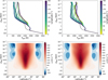 |
Fig. 1 Temperature-pressure (T-p) profiles (top row) at the equatorial region as a function of longitude (colour bar) for the short (left) and long (right) timescale formation simulation. The dashed line shows a polar T–p profile. Zonal mean zonal velocity (bottom row) of the HD 189733b simulation for the short (left) and long (right) timescale formation simulation. |
3.4 Haze production rate
In Fig. 2, we show the solid haze formation rate, ![Mathematical equation: $\[\dot{P}_{\mathrm{h}}\left[\mathrm{g} ~\mathrm{g}^{-1} \mathrm{~s}^{-1}\right]\]$](/articles/aa/full_html/2026/08/aa60641-26/aa60641-26-eq43.png) at the 10−5 bar pressure level for each GCM simulation. Here the effect of the delayed timescale scheme is apparent, with the short timescale assumption confining the haze formation to the dayside of the planet, while the delayed scheme allows a significant portion of the haze particles to form on the nightside hemisphere. The maximum regions of haze formation are also changed, with the short timescale scheme producing maximum haze near the sub-stellar point, while the long timescale haze has its maximum near the western terminator. This is probably due to the western terminator downwelling region advecting precursor material to this pressure layer before it is converted to solid haze.
at the 10−5 bar pressure level for each GCM simulation. Here the effect of the delayed timescale scheme is apparent, with the short timescale assumption confining the haze formation to the dayside of the planet, while the delayed scheme allows a significant portion of the haze particles to form on the nightside hemisphere. The maximum regions of haze formation are also changed, with the short timescale scheme producing maximum haze near the sub-stellar point, while the long timescale haze has its maximum near the western terminator. This is probably due to the western terminator downwelling region advecting precursor material to this pressure layer before it is converted to solid haze.
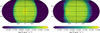 |
Fig. 2 2D latitude-longitude map of the solid haze particle mass mixing ratio formation rate, |
![Mathematical equation: $\[\dot{P}_{\mathrm{h}}\left[\mathrm{g} ~\mathrm{g}^{-1} \mathrm{~s}^{-1} \equiv \mathrm{~s}^{-1}\right]\]$](/articles/aa/full_html/2026/08/aa60641-26/aa60641-26-eq44.png)
3.5 Short formation timescale
In Fig. 3, we present vertical profiles of the moment mixing ratios, haze number density and particle size for the short formation timescale simulation. Our mass mixing ratio results show a similar structure to that of Steinrueck et al. (2023), with values starting from the initial mixing ratios at the formation regions and decreasing with increasing pressure. Our haze formation scheme produces a significant number density of nh > 102 cm−3 at pressures p < 0.1 bar, but small particle sizes of a maximum of ~ 20 nm near the parameterised thermal decomposition pressure.
Figure A.1 shows the 2D latitude-longitude maps of the haze mass mixing ratio and particle sizes at various isobar pressures in the simulation. This shows a very similar 3D global distribution of haze particles to that of Steinrueck et al. (2023), where the mass mixing ratio of the particles follows closely the vertical velocity structure of the atmosphere, with significant regions of higher mass mixing ratio at the western limb of the planet where downwelling from higher altitude occurs (Steinrueck et al. 2023). The particle sizes follow a similar dynamical pattern to the mass mixing ratio, with larger particles generally present in regions of larger mixing ratio and vice versa. This behaviour lines up with Fig. 3, where the number density and particle sizes are inversely related with height. However, this is not always the case, particularly in the upper atmosphere (p < 10−4 bar), where larger mass mixing ratios are correlated with smaller particles. At very low pressures, the collisional timescale is longer and the particle size is influenced more by whether the local flow is upwelling or downwelling. In regions of downwelling, smaller particles from lower pressures are being mixed downwards, and thus the particle size decreases. In regions of upwelling, larger particles from higher pressures are being transported upwards and the average particle size increases. In contrast, deeper in the atmosphere, the collisional timescale is shorter and in regions of enhanced mass mixing ratio, particles will grow faster, leading to a greater correlation between mass mixing ratio and particle size. Overall, our results suggest that the collisional behaviour and overall global structure of the haze particles are a result of a complex interaction of the flow patterns, settling rates and local collisional rates.
3.6 Long formation timescale
In Fig. 4, we present vertical profiles of the moment mixing ratios, haze number density and particle size for the long formation timescale simulation. Here, similar profiles to the short timescale case are seen, but with enhancements of mixing ratios on the nightside of the planet, especially at the western limb regions compared to the short timescale structures. The overall number density profiles are similar between the two cases, but the longer formation timescale produces larger particles, up to ~30 nm in the atmosphere compared to the short timescale ~20 nm.
Figure A.2 shows the latitude-longitude maps of the haze mass mixing ratio and particle sizes at various isobar pressures in the simulation. These show a highly similar pattern to the short timescale results, but with generally more enhancement of particles on the nightside hemisphere, and typically larger particles at each isobar pressure level.
Overall, the long timescale results suggest a generally faster coagulation rate compared to the short timescale simulations and a longer residence time allowing the haze to grow larger before settling out. For the faster coagulation explanation, the increased particle sizes are likely due to an increase in the overall mass mixing ratios at the dynamically convergent east and west limb regions of the atmosphere, which leads to a larger coagulation rate and therefore larger particles. For the longer residence explanation, the delayed formation timescale scheme naturally allows the smallest particles to spread across the globe before colliding and growing, retaining more material before they are dynamically converged and allowed to grow. However, both mechanisms are not fast enough to overcome the natural dynamical timescales of the planet and decouple strongly from the flow, with haze particles still in the nanometre regime.
Our long timescale simulations produce an equatorial banding pattern of the largest particles (≈30 nm), similar to the banding of mass mixing ratio seen by Steinrueck et al. (2021) at 10−2 bar. From our GCMs and the results of Steinrueck et al. (2021), this region dynamically converges the mixing ratio of the haze particles, which in our model enables a larger particle size to be produced. This banding is also seen in the short timescale simulations, but to a lesser extent, suggesting a link between the settling rate of particles and the dynamical structures at this pressure. This is confirmed by Steinrueck et al. (2021), who found larger particles increased the overall mass mixing ratio in this equatorial band compared to smaller particles.
In addition, the correlation between the mass mixing ratio and particle size occurs to a much greater extent at 10−2 bar compared to the lower pressure regions in both the short and long timescale simulations, especially at the equatorial regions. This suggests a dynamical convergence of both moment quantities when haze enters this dynamical layer. This is seen by Steinrueck et al. (2021) and Mak et al. (2025), who also found a strong convergence of the mass mixing ratio of haze at these pressure levels.
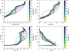 |
Fig. 3 Short formation timescale vertical profiles of the zeroth moment volume mixing ratio, q0 [cm3 cm−3] (top left); first moment mass mixing ratio, q1 [g g−1] (top right); haze particle number density, nh [cm−3] (bottom left); and haze particle radius, rh [nm] (bottom right). Coloured lines denote the longitude (colour bar) at the equatorial region, while the dashed black line denotes a polar region. |
3.7 Post-processing
In this section, we post-process the results of the GCM simulations using the 3D radiative-transfer model gCMCRT (Lee et al. 2022). We produce synthetic transmission spectra and dayside emission spectra to explore the impact of the 3D haze distributions. We assume a well-peaked, lognormal, distribution with geometric standard deviation of σg = 1.05, taking the mean haze particle size (Eq. (5)) in each cell as the median value for the distribution. This helps smooth the Mie theory calculations to avoid strong resonance bump features that can occur when assuming a single particle size.
Figure 5 presents the transmission spectra of our GCM simulation output. In transmission, both our haze timescales simulation results add appreciable opacity to the atmosphere, resulting in muted spectral features across the infrared wavelength regime. The long timescale results produce a more significant source of haze opacity, greatly flattening the spectra. This is expected from our GCM results, where we found that larger thermal feedback effects were present for the long timescale simulation compared to the short timescale, suggesting a large overall haze opacity component. This is probably due to the generally larger particle sizes in the long timescale simulation present across the globe. However, similar to Steinrueck et al. (2023) and Mak et al. (2025), we find that soot particles, without tuning the vertical mixing profiles, cannot fit the observed strong Rayleigh-like slope at optical wavelengths.
Figure 5 also shows the dayside emission spectra in the midinfrared regime, compared to the Inglis et al. (2024) JWST MIRI LRS measurements. We find that the haze particles generally increase the planetary flux due to the increased temperatures on the dayside of the atmosphere from thermal feedback of the haze opacity (Fig. 1). The short timescale simulations show only a slight increase in the dayside emission, showing that the temperature structures are generally similar with and without haze feedback. However, the long timescale simulations show a stronger thermal response, raising the emission spectra by 100–200 ppm across the MIRI LRS wavelength regime. This feedback places the spectrum generally too high compared to the MIRI LRS data from Inglis et al. (2024).
Figure 6 shows the 3D dayside-averaged fractional contribution function for both the short and long timescale simulations for the MIRI LRS wavelength range. Both simulations show similar contribution function contours, with most flux emanating between 0.1 and 0.01 bar. This region is where the maximum haze particle sizes are found (Figs. 3 and 4), so that the dayside emission probes the same pressure range over which the haze opacity and its thermal feedback are strongest. This explains why the long timescale simulation, with its larger particles and stronger upper-atmosphere heating (Fig. 1), produces the elevated dayside flux seen in Fig. 5, while the contribution function itself remains largely unchanged between the two cases: the haze alters the temperature at these levels rather than shifting the levels from which the flux emerges.
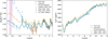 |
Fig. 5 Transmission spectra (left), and dayside emission spectra (right) of our GCM simulations, for the short (blue solid line), and long (orange solid line) haze formation timescales. Dotted green lines show the spectrum before the radiative-feedback from haze was introduced. We include the available transmission spectra for HD 189733b from Cubillos et al. (2023), Sing et al. (2016), and Fu et al. (2024), as well as the MIRI LRS dayside emission data from Inglis et al. (2024) for illustration. |
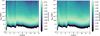 |
Fig. 6 Dayside-averaged 3D contribution functions of the GCM simulations for short (left) and long (right) haze formation timescale simulations. The regions contributing to the emission spectra are similar between each simulation. |
4 Discussion
In this study, we have parameterised the production rate of precursor molecules and a timescale-dependent activation and haze formation scheme. Several laboratory studies have now produced haze formation rates and compositions for sets of exoplanetary conditions (e.g. Hörst et al. 2018; He et al. 2020; Moran et al. 2020; Thompson 2026). Future modelling efforts can attempt to simulate atmospheres that contain similar compositions, but with the haze formation timescales estimated from the available experimental data. This may be more feasible for sub-Neptune modelling where haze formation experiments in sub-Neptune-like atmospheric environments have already been performed in detail (e.g. Hörst et al. 2018). This would be a good test of the modelling approach and provide a useful synergy between laboratory studies and theory.
In this study, we have assumed constant, highly parameterised activation and decay timescales for a generic precursor set of molecules. Deriving temperature- and pressure-dependent rates for a set of precursors using photochemical models (e.g. Tsai et al. 2021), possibly using simplifying methods such as chemical relaxation timescales (e.g. Tsai et al. 2018) may be warranted in the future. These efforts would produce a more chemically consistent haze formation timescale for 3D simulations. Most naturally, chemically consistent 3D kinetic-chemistry models such as mini-chem (Lee et al. 2023) or the Drummond et al. (2020); Zamyatina et al. (2023) scheme, as well as current 2D photochemical modelling efforts (e.g. Tsai et al. 2023b) could be coupled to mini-haze to investigate the effect of 2D/3D precursor molecule distributions on haze particle formation rates. However, for the 3D models, photochemical processes would have to be included before a more fully consistent 3D approach would be feasible.
Lavvas & Koskinen (2017) applied a haze evolution model originally designed for Titan studies (Lavvas et al. 2010) to the atmosphere of HD 209458b and HD 189733b. This uses a 1D bin evolution model to evolve the haze particle size distribution, including collisional growth processes and a similar parameterisation for the height dependent haze formation rate to that used here. Although it is not straightforward to compare 1D simulations with 3D simulations, our results are in good agreement with the structures and particle sizes found by Lavvas & Koskinen (2017) at similar haze particle formation rates. For example, the Lavvas & Koskinen (2017) HD 189733b simulation produces haze particle sizes up to ~20–30 nm for their 10−12 g cm−2 s−1, 0.1 Kzz profile case, which is in line with the GCM results which have an overall similar haze particle formation rate. We suggest that since the particle sizes remain relatively small in this particular haze formation scenario, the monodisperse approximation of the moment method holds well and strong polydisperse components are not important in altering the growth rates significantly. The results from the bin model Gao et al. (2023) suggest some polydisperse behaviour can occur but the bulk of the haze mass is retained in the small particle sizes of <0.1 μm. Overall, the similarity between the vertical haze structures and particle sizes in the complex Lavvas & Koskinen (2017) bin model and our GCM moment approach suggests that our moment method is accurately capturing the salient haze collisional growth processes in the atmosphere.
5 Conclusions
In this study, we presented ‘mini-haze’, a flexible two-moment photochemical haze formation scheme designed for ease of use in time-dependent exoplanet atmosphere simulations. mini-haze evolves the haze particle number density and particle size properties self-consistently, using a coagulation-coalescence approach, going beyond the previous single-sized haze particle studies used by Steinrueck et al. (2021) and Steinrueck et al. (2023). mini-haze is available online on GitHub3.
Inspired by recent 2D kinetic chemistry (Tsai et al. 2023b) and cloud particle condensation models (Powell & Zhang 2024), we proposed a simple activation and decay chemical timescale method to emulate the time evolution and efficiency of precursor molecule conversion into solid haze particles. Through choosing the balance between these timescales, the appropriate conversion efficiency between precursor molecules and haze particles can be naturally included in the model. Our current model used a simple parameterised pressure-dependent haze production rate similar to previous modelling efforts. Our scheme is flexible for future efforts that may self-consistently calculate a production rate based on the 3D time-dependent chemical structure.
In an initial test, we applied our model to simulate a hazy hot Jupiter HD 189733b atmosphere scenario using mini-haze coupled to the Exo-FMS GCM. We examined differences between assuming an instantaneous haze formation timescale and a delayed timescale, approximately half the advective timescale, to allow a component of the haze to form on the nightside hemisphere of the planet. Our chosen precursor formation rate results in maximum haze particle sizes of ~ 2–30 nm, with the 3D distribution of hazes closely following the dominant horizontal dynamical structures and vertical velocity profiles of the atmosphere, as seen in previous 3D hot Jupiter haze particle studies (Steinrueck et al. 2023).
Our transmission spectra results showed muting of spectral features from the presence of haze particles, with the long formation timescale haze producing appreciably more opacity than the short timescale haze formation results. We found the emission spectrum is not affected significantly by the presence of haze particle opacity itself, but the stronger thermal feedback present in the long timescale simulation compared to the short timescale simulation leads to an overall greater planetary flux.
Our current model conforms well with previous 1D studies that used a complex bin haze formation model on the same planet (Lavvas & Koskinen 2017), reproducing similar particle number densities and particle sizes at comparable haze formation rates. The coupled mini-haze and GCM models reproduce well the global haze distribution of studies that used parameterised haze particle sizes (Steinrueck et al. 2021, 2023), with the 3D distribution of haze particles following the similar vertical velocity structures, vertical mixing ratios, thermal feedback effects and overall effect on transmission and emission spectra. While our results are complementary and concordant with Steinrueck et al. (2021), Steinrueck et al. (2023) and Mak et al. (2025), the key advance of mini-haze is that the particle sizes are evolved self-consistently through collisional growth rather than fixed a priori, and that the haze precursor production and conversion efficiency are set by a physically motivated timescale scheme rather than a prescribed solid formation rate.
Overall, mini-haze offers a general, flexible and efficient way of including a haze formation component in time-dependent models of exoplanet atmospheres. mini-haze uses a two-moment method, as well as a simple precursor material to haze particle timescale scheme, to model the production of haze monomers and their subsequent collisional growth across the atmosphere. mini-haze is highly complementary to current and future photochemical models that aim to add a haze formation component to their kinetic chemistry models. Our current methodology including haze formation and evolution, kinetic chemistry and thermal-feedback effects represents a step towards full self-consistency in understanding chemical and haze interactions in exoplanet atmospheres. In a forthcoming paper (Paper II), we will extend the mini-haze framework to cooler sub-Neptune atmospheres and explore how different haze compositions and formation efficiencies shape their 3D spatial distributions and observable spectra.
Acknowledgements
We thank P. Lavvas for making available soot particle optical constants. E.K.H. Lee is supported by the CSH Bernoulli Fellowship. M.E. Steinrueck is supported by a 51 Pegasi b fellowship from the Heising-Simons Foundation. K. Ohno acknowledges support from the JSPS KAKENHI grant numbers JP23K19072 and JP21H01141. X. Zhang acknowledges support from the NSF grant (AST2307463), NASA Exoplanet Research grant (80NSSC22K0236), and the NASA Interdisciplinary Consortia for Astrobiology Research grant (80NSSC21K0597). This work benefited from the 2024 Exoplanet Summer Program in the Other Worlds Laboratory (OWL) at the University of California, Santa Cruz, a program funded by the Heising-Simons Foundation and NASA.
References
- Ackerman, A. S., & Marley, M. S. 2001, ApJ, 556, 872 [Google Scholar]
- Adams, D., Gao, P., de Pater, I., & Morley, C. V. 2019, ApJ, 874, 61 [NASA ADS] [CrossRef] [Google Scholar]
- Addison, B., Wright, D. J., Wittenmyer, R. A., et al. 2019, PASP, 131, 115003 [NASA ADS] [CrossRef] [Google Scholar]
- Agol, E., Cowan, N. B., Knutson, H. A., et al. 2010, ApJ, 721, 1861 [Google Scholar]
- Ahrer, E.-M., Radica, M., Piaulet-Ghorayeb, C., et al. 2025, ApJ, 985, L10 [Google Scholar]
- Amundsen, D. S., Tremblin, P., Manners, J., Baraffe, I., & Mayne, N. J. 2017, A&A, 598, A97 [NASA ADS] [CrossRef] [EDP Sciences] [Google Scholar]
- Arfaux, A., & Lavvas, P. 2024, MNRAS, 530, 482 [NASA ADS] [CrossRef] [Google Scholar]
- Bertrand, T., & Forget, F. 2017, Icarus, 287, 72 [Google Scholar]
- Bohren, C. F., & Huffman, D. R. 1983, Absorption and Scattering of Light by Small Particles (New York: John Wiley & Sons) [Google Scholar]
- Bouchy, F., Udry, S., Mayor, M., et al. 2005, A&A, 444, L15 [EDP Sciences] [Google Scholar]
- Brande, J., Crossfield, I. J. M., Kreidberg, L., et al. 2024, ApJ, 961, L23 [NASA ADS] [CrossRef] [Google Scholar]
- Chandrasekhar, S. 1943, Rev. Mod. Phys., 15, 1 [CrossRef] [Google Scholar]
- Christie, D. A., Mayne, N. J., Gillard, R. M., et al. 2022, MNRAS, 517, 1407 [NASA ADS] [CrossRef] [Google Scholar]
- Chubb, K. L., Tennyson, J., & Yurchenko, S. N. 2020, MNRAS, 493, 1531 [NASA ADS] [CrossRef] [Google Scholar]
- Cohen, M., Palmer, P. I., Paradise, A., Bollasina, M. A., & Tiranti, P. I. 2024, AJ, 167, 97 [NASA ADS] [CrossRef] [Google Scholar]
- Coles, P. A., Yurchenko, S. N., & Tennyson, J. 2019, MNRAS, 490, 4638 [CrossRef] [Google Scholar]
- Corrales, L., Gavilan, L., Teal, D. J., & Kempton, E. M. R. 2023, ApJ, 943, L26 [Google Scholar]
- Cubillos, P. E., Fossati, L., Koskinen, T., et al. 2023, A&A, 671, A170 [NASA ADS] [CrossRef] [EDP Sciences] [Google Scholar]
- Davidson, T. 1993, A Simple and Accurate Method for Calculating Viscosity of Gaseous Mixtures, Report of investigations (Amarillo, TX: U.S. Department of the Interior, Bureau of Mines) [Google Scholar]
- Désert, J.-M., Sing, D., Vidal-Madjar, A., et al. 2011, A&A, 526, A12 [NASA ADS] [CrossRef] [EDP Sciences] [Google Scholar]
- Drummond, B., Hébrard, E., Mayne, N. J., et al. 2020, A&A, 636, A68 [NASA ADS] [CrossRef] [EDP Sciences] [Google Scholar]
- Finnerty, L., Xuan, J. W., Xin, Y., et al. 2024, AJ, 167, 43 [NASA ADS] [CrossRef] [Google Scholar]
- Fleury, B., Gudipati, M. S., Henderson, B. L., & Swain, M. 2019, ApJ, 871, 158 [NASA ADS] [CrossRef] [Google Scholar]
- Fu, G., Welbanks, L., Deming, D., et al. 2024, Nature, 632, 752 [Google Scholar]
- Gao, P., & Benneke, B. 2018, ApJ, 863, 165 [CrossRef] [Google Scholar]
- Gao, P., Thorngren, D. P., Lee, E. K. H., et al. 2020, Nat. Astron., 4, 951 [NASA ADS] [CrossRef] [Google Scholar]
- Gao, P., Piette, A. A. A., Steinrueck, M. E., et al. 2023, ApJ, 951, 96 [NASA ADS] [CrossRef] [Google Scholar]
- Grillmair, C. J., Charbonneau, D., Burrows, A., et al. 2007, ApJ, 658, L115 [NASA ADS] [CrossRef] [Google Scholar]
- Guillot, T., Ida, S., & Ormel, C. W. 2014, A&A, 572, A72 [NASA ADS] [CrossRef] [EDP Sciences] [Google Scholar]
- Hargreaves, R., Gordon, I., Kochanov, R., & Rothman, L. 2019, in EPSC-DPS Joint Meeting 2019, EPSC-DPS2019-919 [Google Scholar]
- Hargreaves, R. J., Gordon, I. E., Rey, M., et al. 2020, ApJS, 247, 55 [NASA ADS] [CrossRef] [Google Scholar]
- Harris, G. J., Tennyson, J., Kaminsky, B. M., Pavlenko, Y. V., & Jones, H. R. A. 2006, MNRAS, 367, 400 [Google Scholar]
- He, C., Hörst, S. M., Lewis, N. K., et al. 2018, AJ, 156, 38 [Google Scholar]
- He, C., Hörst, S. M., Lewis, N. K., et al. 2020, Planet. Sci. J., 1, 51 [Google Scholar]
- He, C., Hörst, S. M., Radke, M., & Yant, M. 2022, Planet. Sci. J., 3, 25 [NASA ADS] [CrossRef] [Google Scholar]
- He, C., Radke, M., Moran, S. E., et al. 2024, Nat. Astron., 8, 182 [Google Scholar]
- Helling, C., Woitke, P., & Thi, W. F. 2008, A&A, 485, 547 [NASA ADS] [CrossRef] [EDP Sciences] [Google Scholar]
- Hörst, S. M., He, C., Lewis, N. K., et al. 2018, Nat. Astron., 2, 303 [Google Scholar]
- Huseby, L., Moran, S. E., Pearson, N., et al. 2025, Planet. Sci. J., 6, 145 [Google Scholar]
- Inglis, J., Batalha, N. E., Lewis, N. K., et al. 2024, ApJ, 973, L41 [NASA ADS] [CrossRef] [Google Scholar]
- Jacobson, M. Z. 2005, Fundamentals of Atmospheric Modeling, 2nd edn. (Cambridge: Cambridge University Press) [Google Scholar]
- Karman, T., Gordon, I. E., van der Avoird, A., et al. 2019, Icarus, 328, 160 [Google Scholar]
- Kataria, T., Showman, A. P., Lewis, N. K., et al. 2013, ApJ, 767, 76 [NASA ADS] [CrossRef] [Google Scholar]
- Kawashima, Y., & Ikoma, M. 2018, ApJ, 853, 7 [NASA ADS] [CrossRef] [Google Scholar]
- Kempton, E. M.-R., Bean, J. L., Louie, D. R., et al. 2018, PASP, 130, 114401 [CrossRef] [Google Scholar]
- Kempton, E. M. R., Zhang, M., Bean, J. L., et al. 2023, Nature, 620, 67 [NASA ADS] [CrossRef] [Google Scholar]
- Khare, B. N., Sagan, C., Arakawa, E. T., et al. 1984, Icarus, 60, 127 [CrossRef] [Google Scholar]
- Kim, J., Mulholland, G., Kukuck, S., & Pui, D. 2005, J. Res. Natl. Inst. Standards Technol., 110, 1 [Google Scholar]
- Kitzmann, D., & Heng, K. 2018, MNRAS, 475, 94 [NASA ADS] [CrossRef] [Google Scholar]
- Knutson, H. A., Lewis, N., Fortney, J. J., et al. 2012, ApJ, 754, 22 [NASA ADS] [CrossRef] [Google Scholar]
- Kreidberg, L., Bean, J. L., Désert, J.-M., et al. 2014, Nature, 505, 69 [Google Scholar]
- Larson, E. J. L., Toon, O. B., West, R. A., & Friedson, A. J. 2015, Icarus, 254, 122 [NASA ADS] [CrossRef] [Google Scholar]
- Lavvas, P., & Koskinen, T. 2017, ApJ, 847, 32 [NASA ADS] [CrossRef] [Google Scholar]
- Lavvas, P., Yelle, R. V., & Griffith, C. A. 2010, Icarus, 210, 832 [NASA ADS] [CrossRef] [Google Scholar]
- Lavvas, P., Paraskevaidou, S., & Arfaux, A. 2024, arXiv e-prints [arXiv:2410.09981] [Google Scholar]
- Lebonnois, S., Burgalat, J., Rannou, P., & Charnay, B. 2012, Icarus, 218, 707 [CrossRef] [Google Scholar]
- Lee, E. K. H. 2023, MNRAS, 524, 2918 [NASA ADS] [CrossRef] [Google Scholar]
- Lee, E. K. H. 2025, A&A, 698, A220 [NASA ADS] [CrossRef] [EDP Sciences] [Google Scholar]
- Lee, E. K. H., & Ohno, K. 2025, A&A, 695, A111 [NASA ADS] [CrossRef] [EDP Sciences] [Google Scholar]
- Lee, E. K. H., Parmentier, V., Hammond, M., et al. 2021, MNRAS, 506, 2695 [NASA ADS] [CrossRef] [Google Scholar]
- Lee, E. K. H., Wardenier, J. P., Prinoth, B., et al. 2022, ApJ, 929, 180 [NASA ADS] [CrossRef] [Google Scholar]
- Lee, E. K. H., Tsai, S.-M., Hammond, M., & Tan, X. 2023, A&A, 672, A110 [NASA ADS] [CrossRef] [EDP Sciences] [Google Scholar]
- Lee, E. K. H., Tan, X., & Tsai, S.-M. 2024, MNRAS, 529, 2686 [NASA ADS] [CrossRef] [Google Scholar]
- Li, G., Gordon, I. E., Rothman, L. S., et al. 2015, ApJS, 216, 15 [NASA ADS] [CrossRef] [Google Scholar]
- Mak, M. T., Mayne, N. J., Sergeev, D. E., et al. 2023, J. Geophys. Res. (Atmos.), 128, e2023JD039343 [Google Scholar]
- Mak, M. T., Sergeev, D. E., Mayne, N., et al. 2024, MNRAS, 529, 3971 [Google Scholar]
- Mak, M. T., Sergeev, D. E., Mayne, N. J., et al. 2025, MNRAS, 542, 1873 [Google Scholar]
- Malsky, I., Rauscher, E., Stevenson, K., et al. 2025, AJ, 169, 221 [Google Scholar]
- Mann, G. W., Carslaw, K. S., Spracklen, D. V., et al. 2010, Geosci. Model Dev.t, 3, 519 [Google Scholar]
- Moosmüller, H., & Sorensen, C. M. 2018, J. Quant. Spec. Radiat. Transf., 219, 333 [CrossRef] [Google Scholar]
- Moran, S. E., Hörst, S. M., Vuitton, V., et al. 2020, Planet. Sci. J., 1, 17 [NASA ADS] [CrossRef] [Google Scholar]
- Morley, C. V., Fortney, J. J., Kempton, E. M. R., et al. 2013, ApJ, 775, 33 [CrossRef] [Google Scholar]
- Morley, C. V., Fortney, J. J., Marley, M. S., et al. 2015, ApJ, 815, 110 [NASA ADS] [CrossRef] [Google Scholar]
- Morán, J. 2022, Fractal Fract., 6, 529 [Google Scholar]
- Ohno, K. 2024, ApJ, 977, 188 [Google Scholar]
- Ohno, K., & Kawashima, Y. 2020, ApJ, 895, L47 [NASA ADS] [CrossRef] [Google Scholar]
- Ohno, K., & Okuzumi, S. 2017, ApJ, 835, 261 [NASA ADS] [CrossRef] [Google Scholar]
- Ohno, K., & Okuzumi, S. 2018, ApJ, 859, 34 [Google Scholar]
- Ohno, K., Okuzumi, S., & Tazaki, R. 2020, ApJ, 891, 131 [Google Scholar]
- Ohno, K., Schlawin, E., Bell, T. J., et al. 2025, ApJ, 979, L7 [Google Scholar]
- Owen, J. E., & Murray-Clay, R. A. 2025, MNRAS, 543, 587 [Google Scholar]
- Pentsak, E. O., Murga, M. S., & Ananikov, V. P. 2024, ACS Earth Space Chem., 8, 798 [Google Scholar]
- Pesciotta, C., Hörst, S. M., Radke, M. J., et al. 2026, ApJ, 1002, 221 [Google Scholar]
- Polyansky, O. L., Kyuberis, A. A., Zobov, N. F., et al. 2018, MNRAS, 480, 2597 [NASA ADS] [CrossRef] [Google Scholar]
- Pont, F., Sing, D. K., Gibson, N. P., et al. 2013, MNRAS, 432, 2917 [NASA ADS] [CrossRef] [Google Scholar]
- Powell, D., & Zhang, X. 2024, ApJ, 969, 5 [NASA ADS] [CrossRef] [Google Scholar]
- Radhakrishnan, K., & Hindmarsh, A. C. 1993, Description and use of LSODE, the Livemore Solver for Ordinary Differential Equations, Tech. rep., Lawrence Livermore National Laboratory (LLNL), Livermore, CA [Google Scholar]
- Rosner, D. E. 2012, Transport Processes in Chemically Reacting Flow Systems (New York: Dover Publications) [Google Scholar]
- Rossow, W. B. 1978, Icarus, 36, 1 [NASA ADS] [CrossRef] [Google Scholar]
- Sato, T., Okuzumi, S., & Ida, S. 2016, A&A, 589, A15 [NASA ADS] [CrossRef] [EDP Sciences] [Google Scholar]
- Schaaf, S. A. 1963, Handb. Phys., 3, 591 [Google Scholar]
- Schlawin, E., Ohno, K., Bell, T. J., et al. 2024, ApJ, 974, L33 [Google Scholar]
- Sing, D. K., Fortney, J. J., Nikolov, N., et al. 2016, Nature, 529, 59 [Google Scholar]
- Steinrueck, M. E., Showman, A. P., Lavvas, P., et al. 2021, MNRAS, 504, 2783 [NASA ADS] [CrossRef] [Google Scholar]
- Steinrueck, M. E., Koskinen, T., Lavvas, P., et al. 2023, ApJ, 951, 117 [NASA ADS] [CrossRef] [Google Scholar]
- Steinrueck, M. E., Parmentier, V., Kreidberg, L., et al. 2025, ApJ, 985, 98 [Google Scholar]
- Teske, J., Batalha, N. E., Wallack, N. L., et al. 2025, AJ, 169, 249 [Google Scholar]
- Thompson, M. A. 2026, Ap&SS, 371, 33 [Google Scholar]
- Toon, O. B., McKay, C. P., Ackerman, T. P., & Santhanam, K. 1989, J. Geophys. Res., 94, 16287 [Google Scholar]
- Tsai, S.-M., Kitzmann, D., Lyons, J. R., et al. 2018, ApJ, 862, 31 [NASA ADS] [CrossRef] [Google Scholar]
- Tsai, S.-M., Malik, M., Kitzmann, D., et al. 2021, ApJ, 923, 264 [NASA ADS] [CrossRef] [Google Scholar]
- Tsai, S.-M., Lee, E. K. H., & Pierrehumbert, R. 2022, A&A, 664, A82 [NASA ADS] [CrossRef] [EDP Sciences] [Google Scholar]
- Tsai, S.-M., Lee, E. K. H., Powell, D., et al. 2023a, Nature, 617, 483 [CrossRef] [Google Scholar]
- Tsai, S.-M., Moses, J. I., Powell, D., & Lee, E. K. H. 2023b, ApJ, 959, L30 [NASA ADS] [CrossRef] [Google Scholar]
- Wallack, N. L., Batalha, N. E., Alderson, L., et al. 2024, AJ, 168, 77 [NASA ADS] [CrossRef] [Google Scholar]
- Woitke, P., & Helling, C. 2003, A&A, 399, 297 [NASA ADS] [CrossRef] [EDP Sciences] [Google Scholar]
- Woitke, P., Helling, C., Hunter, G. H., et al. 2018, A&A, 614, A1 [NASA ADS] [CrossRef] [EDP Sciences] [Google Scholar]
- Yu, X., He, C., Zhang, X., et al. 2021, Nat. Astron., 5, 822 [NASA ADS] [CrossRef] [Google Scholar]
- Yurchenko, S. N., Mellor, T. M., Freedman, R. S., & Tennyson, J. 2020, MNRAS, 496, 5282 [NASA ADS] [CrossRef] [Google Scholar]
- Zamyatina, M., Hébrard, E., Drummond, B., et al. 2023, MNRAS, 519, 3129 [Google Scholar]
Appendix A Longitude-latitude maps
In this Appendix, we present the latitude-longitude maps of each simulation at various pressure levels for the short (Fig. A.1) and long (Fig. A.2) haze formation timescales.
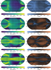 |
Fig. A.1 Haze mass mixing ratio, q1 [g g−1] (left column); and haze particle size, rh [nm] (right column); for the short formation timescale simulation at 10−5 bar (top row), 10−4 bar (second row), 10−3 bar (third row) and 10−2 bar (bottom row) pressure levels. The sub-stellar point is located at (0°, 0°). |
All Tables
Adopted Exo-FMS simulation parameters for the hazy HD 189733b hot Jupiter scenario.
All Figures
|
Fig. 1 Temperature-pressure (T-p) profiles (top row) at the equatorial region as a function of longitude (colour bar) for the short (left) and long (right) timescale formation simulation. The dashed line shows a polar T–p profile. Zonal mean zonal velocity (bottom row) of the HD 189733b simulation for the short (left) and long (right) timescale formation simulation. |
| In the text | |
|
Fig. 2 2D latitude-longitude map of the solid haze particle mass mixing ratio formation rate, |
| In the text | |
|
Fig. 3 Short formation timescale vertical profiles of the zeroth moment volume mixing ratio, q0 [cm3 cm−3] (top left); first moment mass mixing ratio, q1 [g g−1] (top right); haze particle number density, nh [cm−3] (bottom left); and haze particle radius, rh [nm] (bottom right). Coloured lines denote the longitude (colour bar) at the equatorial region, while the dashed black line denotes a polar region. |
| In the text | |
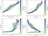 |
Fig. 4 Same as Fig. 3 but for the long haze formation timescale. |
| In the text | |
|
Fig. 5 Transmission spectra (left), and dayside emission spectra (right) of our GCM simulations, for the short (blue solid line), and long (orange solid line) haze formation timescales. Dotted green lines show the spectrum before the radiative-feedback from haze was introduced. We include the available transmission spectra for HD 189733b from Cubillos et al. (2023), Sing et al. (2016), and Fu et al. (2024), as well as the MIRI LRS dayside emission data from Inglis et al. (2024) for illustration. |
| In the text | |
|
Fig. 6 Dayside-averaged 3D contribution functions of the GCM simulations for short (left) and long (right) haze formation timescale simulations. The regions contributing to the emission spectra are similar between each simulation. |
| In the text | |
|
Fig. A.1 Haze mass mixing ratio, q1 [g g−1] (left column); and haze particle size, rh [nm] (right column); for the short formation timescale simulation at 10−5 bar (top row), 10−4 bar (second row), 10−3 bar (third row) and 10−2 bar (bottom row) pressure levels. The sub-stellar point is located at (0°, 0°). |
| In the text | |
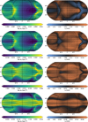 |
Fig. A.2 Same as Fig. A.1 but for the long haze formation timescale. |
| In the text | |
Current usage metrics show cumulative count of Article Views (full-text article views including HTML views, PDF and ePub downloads, according to the available data) and Abstracts Views on Vision4Press platform.
Data correspond to usage on the plateform after 2015. The current usage metrics is available 48-96 hours after online publication and is updated daily on week days.
Initial download of the metrics may take a while.