| Issue |
A&A
Volume 709, May 2026
|
|
|---|---|---|
| Article Number | L15 | |
| Number of page(s) | 9 | |
| Section | Letters to the Editor | |
| DOI | https://doi.org/10.1051/0004-6361/202660217 | |
| Published online | 12 May 2026 | |
Letter to the Editor
A tidally detached super Neptune on a strongly misaligned retrograde orbit
1
Centro di Ateneo di Studi e Attività Spaziali “G. Colombo” – Università degli Studi di Padova, Via Venezia 15, IT-35131 Padova, Italy
2
INAF – Osservatorio Astronomico di Padova, Vicolo dell’Osservatorio 5, IT-35122 Padova, Italy
3
Dipartimento di Fisica e Astronomia “Galileo Galilei”, Università di Padova, Vicolo dell’Osservatorio 3, IT-35122 Padova, Italy
4
INAF – Osservatorio Astrofisico di Catania, Via Santa Sofia 78, IT-95123 Catania, Italy
5
Dipartimento di Fisica e Astronomia, Università di Padova, Via Marzolo 8, IT-35121 Padova, Italy
6
INAF – Osservatorio Astronomico di Roma, Monte Porzio Catone, IT-00043, Roma, Italy
7
Fundación Galileo Galilei-INAF, Rambla José Ana Fernandez Pérez 7, ES-38712 Breña Baja, Spain
8
INAF – Osservatorio Astronomico di Palermo, Piazza del Parlamento 1, IT-90134 Palermo, Italy
9
INAF – Osservatorio Astrofisico di Torino, Via Osservatorio 20, IT-10025 Pino Torinese, Italy
10
Carnegie Science Observatories, CA 91101 Pasadena, USA
11
Department of Astronomy, University of Wisconsin, 475 N. Charter Str., WI 53706 Madison, USA
12
Dipartimento di Matematica e Fisica, Università Roma Tre, Via della Vasca Navale 84, IT-00146 Roma, Italy
13
Department of Physics and Kavli Institute for Astrophysics and Space Research, MIT, MA 02139 Cambridge, USA
★ Corresponding author: This email address is being protected from spambots. You need JavaScript enabled to view it.
Received:
2
April
2026
Accepted:
20
April
2026
Abstract
The obliquity between a planet’s orbital axis and its host star’s spin axis provides crucial insights into planetary formation and migration. Planets with scaled semi-major axes (a/R★) large enough to be unaffected by tidal alterations (‘tidally detached’) offer a unique opportunity to study the original obliquity in which the system formed. We therefore observed TOI-1710 b (a/R★ ≈ 36) in transit using HARPS-N + GIANO-B, collecting high-precision radial velocities to measure the Rossiter-McLaughlin effect. Spectral analysis of the Hα and HeI triple lines was also pursued to evaluate atmospheric photoevaporation. Using our knowledge of the star rotation period (21.5 ± 0.2 d), we estimated a true obliquity of ψ = 149+11−10 deg, which indicates a retrograde motion, thus placing TOI-1710 b among the most misaligned systems – and making it the only one known to orbit a cool star in retrograde motion. The strong misalignment favours a high-eccentricity migration (HEM) origin for this low-density super-Neptune planet in the savanna region, challenging previous findings that claimed a minor role of HEM in this period-radius(-density) domain. Moreover, the strong misalignment and lack of a detected close stellar companion suggest a purely planetary post-migration misalignment, likely due to planet-planet scattering followed by planet-planet Kozai-Lidov oscillations and tidal circularisation.
Key words: techniques: radial velocities / planets and satellites: dynamical evolution and stability / planet-star interactions
© The Authors 2026
 Open Access article, published by EDP Sciences, under the terms of the Creative Commons Attribution License (https://creativecommons.org/licenses/by/4.0), which permits unrestricted use, distribution, and reproduction in any medium, provided the original work is properly cited.
This article is published in open access under the Subscribe to Open model. This email address is being protected from spambots. You need JavaScript enabled to view it. to support open access publication.
1. Introduction
The architecture of planetary systems encodes information about their formation and migration histories. In this context, measuring the orbital obliquity – the angle between a planet’s orbital angular momentum and its host star spin angular momentum – has proven to be fundamental. The sky-projected obliquity (λ) can be detected with in-transit radial velocities (RVs) via the Rossiter-McLaughlin (RM) effect (e.g. Queloz et al. 2000). This can be translated into the 3D orbital obliquity (ψ) with respect to the stellar rotation axis thanks to the knowledge of a reliable stellar rotation period, projected rotational velocity, and stellar radius, hence stellar inclination (i★). Star-planet tidal interactions may alter the obliquity, and close-in planets orbiting stars a few gigayears old with sizeable convective envelopes are expected to show aligned configurations, making the formation mechanism inaccessible. By observing systems with scaled orbital semi-major axes (a/R★) large enough to avoid tidal alterations to their obliquity, we can access the original obliquity configuration in which the system formed (e.g. Wright et al. 2023). These systems are categorised as ‘tidally detached’ (Rice et al. 2021), as the tidal alignment timescale is longer than the age of the system (Lai 2012).
Super-Neptune exoplanets (4 R⊕ ≲ Rp ≲ 8 R⊕) are an intriguing population for studies of planetary formation and evolution. While the dearth of short-period (P ≲ 3 d) super-Neptune exoplanets is well-known as the ‘Neptune desert’ (e.g. Mazeh et al. 2016, and references therein), only recent studies have shown additional structures on the Neptune planet distribution. Neptunes pile up in a ‘ridge’ (3 − 6 d, Castro-González et al. 2024a) before falling off into the ‘savanna’ (P ≳ 6 d, Bourrier et al. 2023). Properties such as bulk densities, eccentricities, and host-star metallicities change significantly within the desert, ridge, and savanna, indicating that these sub-populations likely have different formation and migration histories (e.g. Armstrong et al. 2020; Naponiello et al. 2023; Vissapragada & Behmard 2025). To validate a complete theory, it is necessary to determine not only the role of different migration pathways but also that of atmospheric evaporation. It is still unknown whether the transition from quiescent to hydrodynamical escape occurs within the desert or the ridge or further out into the savanna (Bourrier et al. 2025).
We present a new study of the ∼24-day orbit super-Neptune TOI-1710 b (König et al. 2022; Polanski et al. 2024; Orell-Miquel et al. 2024, K22, OM24) located in the savanna. The large a/R★ (≈36) makes it tidally detached, which means that we can access the original unaltered obliquity configuration and investigate the processes that led to its current architecture.
2. Observations and data reduction
We observed TOI-1710 (mV = 9.5) with the TNG telescope in the GIARPS observing mode (Claudi et al. 2017, and references therein), which enabled simultaneous measurement of high-resolution spectra in the optical (0.39 − 0.69 μm, R ∼ 115 000, HARPS-N) and the near-infrared (0.95 − 2.45 μm, R ∼ 50 000, GIANO-B). We collected in-transit (5.2 hours) and suitable off-transit (2 hours) observations on February 2, 2024, obtaining 42 spectra with texp= 600 s. We used the ESPRESSO Data Reduction Software (DRS; Pepe et al. 2021) v3.2.0, optimised for HARPS-N (Dumusque et al. 2021), and computed the RVs using the cross-correlation function (CCF) method (Pepe et al. 2002) with a G2 mask. We proceeded in this way to extract the RVs (including the literature data), rather than using a template matching pipeline, because our RM model simulates the CCF anomaly caused by the transiting planet.
The Transiting Exoplanet Survey Satellite (TESS) observed TOI-1710 at 2 min cadence in sectors 19, 20, 26, 40, 53, 60, 73, and 79. We extracted light curves using the PATHOS approach (Nardiello et al. 2020). The TESS sectors 73 and 79, previously unpublished, were essential for refining the transit ephemeris of TOI-1710 b (uncertainty of about 1 min on the night of February 2) required for the RM modelling.
3. Analysis
We simultaneously modelled each TESS sector with all the HARPS-N off-transit RVs (from König et al. 2022; Orell-Miquel et al. 2024, and Sect. 2) and our in-transit RV anomaly. A detailed description of our analysis can be found in Appendix A. The best-fit RM and RV models are shown in Figs. 1 and A.1, and the fitting values are provided in Tables H.1 and H.3. We also did a transmission spectroscopy analysis to search for signs of atmospheric photoevaporation; the results and methodology are summarised in Appendix G.
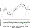 |
Fig. 1. Rossiter-McLaughlin fit to the in-transit RV of TOI-1710 b. Top: Best-fit (line) over the RVs data, corrected for the Keplerian RV curve and systemic RV. Bottom: Residuals of the fit. |
3.1. Transit ephemeris and planet parameters refinement
We refined the planetary radius, mass, and bulk density, achieving precisions of 2%, 22%, and 22%, respectively. The radius value agrees with all previous studies, whereas our mass is 1σ lower. This could be attributed to an improved treatment of stellar parameters and activity, as K22 did not account for its presence, OM24 used an incorrect stellar density value in the modelling, and Polanski et al. (2024) mentioned their methodology may provide inaccurate mass estimates for active stars. Such precisions are necessary to constrain the planetary composition, i.e. the planet mass fraction of rock, gas, and water, and to enable comparative atmospheric studies across the Neptune desert, ridge, and savanna. The low bulk density (ρb = 0.50 ± 0.11 g cm−3) of TOI-1710 b is consistent with the trend noted in Castro-González et al. (2024b), where planets in the savanna typically have ρb < 1 g cm−3. Based on this threshold, the authors identified a dichotomy in the Neptunian population, separating low-density ‘fluffy’ planets, such as TOI-1710 b, from higher density (‘dense’) planets.
3.2. Rossiter-McLaughlin effect
From the Bayesian modelling of the RM effect, we obtained a sky-projected obliquity of  deg. Then thanks to the estimation of a reliable stellar rotation period (Prot = 21.5 ± 0.2 d,
  km s−1; see Appendix B and v sin i★ extraction details in K22, where the HARPS-N and SOPHIE spectra indicate v sin i★ > 2 km s−1), we translated λ into the true 3D orbital obliquity (ψ). We did so by sampling from the posterior distributions of λ, of stellar inclination (i★) and of planetary orbital inclination (ip) and by using Eq. (7) from Winn et al. (2007) (cos ψ = sin i★ cos λ sin ip + cos i★ cos ip) to estimate
  deg. This result confirms the retrograde motion, and it favours a strongly misaligned orbit (see Fig. 1).
4. Discussion
4.1. The retrograde orbit of TOI-1710 b
The 3D obliquity of TOI-1710 b stands in the top 1% of all obliquity measurements when compared alongside those of each known system with a ψ measurement (cf. TEPCat, Southworth 2011) in a polar plot (Fig. 2). Moreover, among the planets orbiting cool stars (Teff < 6250 K, the Kraft break, Kraft 1967), TOI-1710 b has the largest ψ – and it is the only one orbiting a cool star known indicating a retrograde motion with certainty. TOI-1710 b is located slightly above the group of misaligned systems with polar orbits that have ψ in the range 80–125 deg (Albrecht et al. 2021; Attia et al. 2023), and it supports the trend noted in Mantovan et al. (2024) that all planets orbiting cool stars in polar (or larger misalignment) orbits have scaled distances of a/R★ > 10. This trend may support that only such cool star, tidally detached systems have preserved their original misalignments, while those with small a/R★ (orbiting cool stars) have either been tidally realigned or aligned from birth.
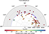 |
Fig. 2. True obliquity of known exoplanets vs. host star effective temperature. TOI-1710 b is indicated by a star. The a/R★ is colour-coded. The shaded region denotes Teff > 6250 K. Data: TEPCat and the NASA Exoplanet Archive as of February 2026. |
The highly misaligned retrograde orbit of TOI-1710 b favours a high-eccentricity migration (HEM, Rasio & Ford 1996; Wu & Murray 2003; Marzari et al. 2006) scenario for this fluffy super-Neptune in the savanna (Fig. 3). This finding seems to disfavour previous hypotheses (Castro-González et al. 2024b; Bourrier et al. 2025) that most fluffy planets – i.e. those in the savanna – reached their locations via disc-driven migrations (Lin et al. 1996), whereas the HEM primarily happened in dense Neptunes, bringing them to the ridge and desert. The characteristics of TOI-1710 b instead suggest that fluffy planets formed beyond the ice line may undergo HEM, possibly triggered by a phase of planet–planet scattering, and reach misaligned orbits without losing their envelopes. This scenario could indicate that HEM may play a role in planetary migration across the entire Neptune period range and over a wider density range. TOI-1710 b is also the longest-period Neptune with a known ψ.
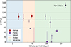 |
Fig. 3. True obliquity of super-Neptunes vs. orbital period. Planetary densities are differentiated by colour and eccentricities by size. The shaded areas separate the desert, ridge, and savanna. |
4.2. Wide binary companion and dynamical implications
Previous high-resolution imaging studies have revealed no close companions within 1.2″ (and from the diffraction limit of 20 mas) and down to contrast limits of Δmag = 5.5–7 2024AA...684A..96O. This corresponds to physical separations of approximately 1.6–97 au, considering the distance of TOI-1710 from the Earth (d = 81 pc). On the other hand, OM24 and González-Payo et al. (2024) confirmed the presence of a wide binary companion located 44.5″ away – originally reported in Mason et al. (2001). Using the Gaia DR3 parallax (Gaia Collaboration 2023), this angular separation translates to a projected distance of about 3600 au. We followed Sozzetti et al. (2023) and conducted a sensitivity analysis of Gaia DR3 astrometry for companions based on the re-normalised unit weight error statistic (RUWE; Lindegren et al. 2021). Such companions would have produced excess residuals in Gaia DR3 astrometry, resulting in a RUWE larger than that measured for TOI-1710 (0.94, compatible with a single-star model). We can rule out brown dwarf companions within 8–10 au, while the sensitivity to super-Jovian companions is limited to 3–4 au. However, the latter can be excluded due to the low peak-to-peak RV residuals (∼4 m s−1), which would only translate to sub-Jovian masses at 4 au (see Appendices F and H).
These findings are crucial to placing constraints on the formation and dynamical history of TOI-1710 b. Highly misaligned retrograde orbits typically originate from dynamical mechanisms involving a close stellar companion (e.g. Marzari & Thebault 2019; Albrecht et al. 2022). As a consequence, we can likely rule out primordial misalignment scenarios for TOI-1710 b since only a protoplanetary disc tilt induced by a close companion (see e.g. Hjorth et al. 2021) would produce the observed ψ. It is worth noting that, provided there is a significant mutual inclination between the disc and the binary orbit, even distant stellar companions can misalign the orbital plane of a disc in less than its lifetime (Batygin 2012). However, the nodal recession period of the disc scales approximately as τdisc ∝ a′3/M′, with a′ being the binary separation and M′ as the companion mass. Therefore, scaling the result of Batygin (2012) for a′ = 500 au and M′ = 1 M⊙ (i.e. 1.8 Myr) to the parameters of TOI-1710 B (a′ = 3600 au and M′≈0.4 M⊙) would imply a much longer timescale (> 500 Myr) than the disc lifetime.
We therefore investigated post-formation mechanisms. Two dynamical processes (or the interplay between them) could explain the observed retrograde orbit: Kozai-Lidov cycles (Wu & Murray 2003) and planet-planet scattering (Marzari et al. 2006). In particular, Kozai-Lidov cycles, especially when the distant companion is on an eccentric orbit (Naoz 2016), have been proposed as the most likely explanations for the retrograde orbits observed in all systems with ψ greater than 120 deg: WASP-131 (Doyle et al. 2023), K2-290 (Hjorth et al. 2021), and KELT-19 (Kawai et al. 2024), all of which have close stellar companions at separations of 38, 110, and 160 au.
In the case of K2-290, Best & Petrovich (2022) discussed the role of a wide binary companion in setting the initial conditions for secular interactions and hence the observed orbital misalignment. However, even in this scenario, the nearby companion at 110 au plays a critical role. Similar to the mechanism proposed for K2-290, Yang et al. (2025) introduced the ‘eccentricity cascade’ non-secular evolution mechanism to explain the retrograde orbit of HAT-P-7 b. However, even this mechanism involving a wide binary requires an intermediate close-orbit stellar companion. For TOI-1710 b, in the absence of such a close companion, we estimated the timescale that Kozai-Lidov oscillations would require if triggered by the wide stellar companion TOI-1710 B alone. We found a timescale of the order of 2 × 10¹⁰ years, making this scenario highly unlikely. On the other hand, a planet-planet Kozai-Lidov cycle involving a hypothetical giant planet at 30 au would yield a much shorter timescale of about 107 years. However, this scenario requires the presence of a second planet in an eccentric, misaligned, and relatively nearby orbit (though this has not been detected yet in the RVs; see Appendix E), which could be the result of planet-planet scattering. We note that in its present orbital configuration, the timescale for apsidal precession (driven primarily by general relativity) is of the order of 3.7 × 10⁵ yr (Mardling & Lin 2002), and this is much shorter than the Kozai-Lidov timescale. Therefore, Kozai-Lidov oscillations could only have played a role in the orbital evolution of TOI-1710 b if it migrated from a more distant location, where the precession timescale would have been longer than the Kozai-Lidov oscillation timescale.
Taken together, these constraints suggest a complex formation history for TOI-1710 b. One possible hypothesis is a multi-step dynamical evolution with planet-planet scattering (or a stellar fly-by, e.g. Malmberg et al. 2011) followed by secular Kozai-Lidov cycles, which may have led to inward migration due to tidal interaction with the star. The two planets could have formed at wide separations from the host star and interacted with each other, and the inner one could have migrated via HEM to arrive at the final orbit in its current misaligned configuration. A notable analogue might be HD80606 b (Naef et al. 2001), a highly eccentric planet in the midst of a HEM, where planet-planet Kozai (Nagasawa et al. 2008) is favoured over star-planet Kozai (Winn et al. 2009) due to the wide separation (∼1200 au) of its stellar companion. Our findings support the hypothesis that both super-Neptune and single-star systems are primordially aligned and may become misaligned during the post-disc phase (see Radzom et al. 2024, 2025).
5. Key findings
-
TOI-1710 b is a tidally detached planet on a strongly misaligned (top 1% of all ψ) retrograde orbit and the only one known to orbit a cool star in retrograde motion with accessible ψ. It is a ‘fluffy’ super-Neptune and the longest-period one with a ψ measurement, and it is also the only one with a retrograde orbit. This is a likely signature of HEM.
-
The HEM mechanism could play a role in the planetary migration of Neptune planets over a wide period (ridge and savanna) and density range. This finding contradicts previous indications that such a mechanism plays only a minor role in shaping the Neptune savanna – more specifically, that of fluffy Neptunes – and will help improve complete migration models.
-
TOI-1710 has a wide stellar companion but lacks close ones, thus favouring a post-formation origin for the observed misalignment over a primordial one. All other systems with ψ > 120 deg instead have a close stellar companion.
-
While retrograde orbits are typically attributed to star-planet Kozai migration induced by an originally misaligned close stellar companion, our work proposes a distinct, purely planetary formation history. The retrograde orbit of TOI-1710 b is most likely the result of planet-planet scattering followed by secular planet-planet Kozai-Lidov oscillations and a final orbit circularisation due to tidal dissipation inside the planet.
Data availability
Table A.1 is available at the CDS via https://cdsarc.cds.unistra.fr/viz-bin/cat/J/A+A/709/L15
Acknowledgments
Based on observations made with the Italian Telescopio Nazionale Galileo (TNG) operated by the Fundación Galileo Galilei (FGG) of the Istituto Nazionale di Astrofisica (INAF) at the Observatorio del Roque de los Muchachos (La Palma, Canary Islands, Spain). This paper includes data collected by the TESS mission. Funding for the TESS mission is provided by the NASA Science Mission directorate. LN and LM acknowledge the financial contribution from the INAF Large Grant 2023 ‘EXODEMO’. L.M. acknowledges financial support from BIRD funds-PRD 2025, DFA-University of Padova.
References
- Albrecht, S. H., Marcussen, M. L., Winn, J. N., et al. 2021, ApJ, 916, L1 [NASA ADS] [CrossRef] [Google Scholar]
- Albrecht, S. H., Dawson, R. I., & Winn, J. N. 2022, PASP, 134, 082001 [NASA ADS] [CrossRef] [Google Scholar]
- Almeida-Fernandes, F., & Rocha-Pinto, H. J. 2018, MNRAS, 476, 184 [Google Scholar]
- Armstrong, D. J., Lopez, T. A., Adibekyan, V., et al. 2020, Nature, 583, 39 [Google Scholar]
- Attia, M., Bourrier, V., Eggenberger, P., et al. 2021, A&A, 647, A40 [NASA ADS] [CrossRef] [EDP Sciences] [Google Scholar]
- Attia, M., Bourrier, V., Delisle, J. B., & Eggenberger, P. 2023, A&A, 674, A120 [NASA ADS] [CrossRef] [EDP Sciences] [Google Scholar]
- Batygin, K. 2012, Nature, 491, 418 [NASA ADS] [CrossRef] [Google Scholar]
- Best, S., & Petrovich, C. 2022, ApJ, 925, L5 [NASA ADS] [CrossRef] [Google Scholar]
- Biazzo, K., D’Orazi, V., Desidera, S., et al. 2022, A&A, 664, A161 [NASA ADS] [CrossRef] [EDP Sciences] [Google Scholar]
- Bourrier, V., Lovis, C., Beust, H., et al. 2018, Nature, 553, 477 [NASA ADS] [CrossRef] [Google Scholar]
- Bourrier, V., Attia, M., Mallonn, M., et al. 2023, A&A, 669, A63 [NASA ADS] [CrossRef] [EDP Sciences] [Google Scholar]
- Bourrier, V., Steiner, M., Castro-González, A., et al. 2025, A&A, 701, A190 [NASA ADS] [CrossRef] [EDP Sciences] [Google Scholar]
- Castro-González, A., Bourrier, V., Lillo-Box, J., et al. 2024a, A&A, 689, A250 [NASA ADS] [CrossRef] [EDP Sciences] [Google Scholar]
- Castro-González, A., Lillo-Box, J., & Armstrong, D. J., et al. 2024b, A&A, 691, A233 [Google Scholar]
- Cegla, H. M., Lovis, C., Bourrier, V., et al. 2016, A&A, 588, A127 [NASA ADS] [CrossRef] [EDP Sciences] [Google Scholar]
- Claudi, R., Benatti, S., Carleo, I., et al. 2017, Eur. Phys. J. Plus, 132, 364 [NASA ADS] [CrossRef] [Google Scholar]
- Cochran, W. D., Fabrycky, D. C., Torres, G., et al. 2011, ApJS, 197, 7 [NASA ADS] [CrossRef] [Google Scholar]
- D’Arpa, M. C., Guilluy, G., Mantovan, G., et al. 2024, A&A, 692, A77 [Google Scholar]
- Dawson, R. I., & Johnson, J. A. 2018, ARA&A, 56, 175 [Google Scholar]
- Delisle, J. B., Hara, N., & Ségransan, D. 2020, A&A, 638, A95 [EDP Sciences] [Google Scholar]
- Delisle, J. B., Unger, N., Hara, N. C., & Ségransan, D. 2022, A&A, 659, A182 [NASA ADS] [CrossRef] [EDP Sciences] [Google Scholar]
- Doyle, L., Cegla, H. M., Anderson, D. R., et al. 2023, MNRAS, 522, 4499 [NASA ADS] [CrossRef] [Google Scholar]
- Dumusque, X., Cretignier, M., Sosnowska, D., et al. 2021, A&A, 648, A103 [NASA ADS] [CrossRef] [EDP Sciences] [Google Scholar]
- Eastman, J., Gaudi, B. S., & Agol, E. 2013, PASP, 125, 83 [Google Scholar]
- Foreman-Mackey, D. 2018, RNAAS, 2, 31 [NASA ADS] [Google Scholar]
- Foreman-Mackey, D., Hogg, D. W., Lang, D., et al. 2013, PASP, 125, 306 [NASA ADS] [CrossRef] [Google Scholar]
- Foreman-Mackey, D., Agol, E., Ambikasaran, S., et al. 2017, AJ, 154, 220 [NASA ADS] [CrossRef] [Google Scholar]
- Gaia Collaboration (Vallenari, A., et al.) 2023, A&A, 674, A1 [NASA ADS] [CrossRef] [EDP Sciences] [Google Scholar]
- Ginzburg, S., & Sari, R. 2017, MNRAS, 464, 3937 [Google Scholar]
- González-Payo, J., Caballero, J. A., Gorgas, J., et al. 2024, A&A, 689, A302 [NASA ADS] [CrossRef] [EDP Sciences] [Google Scholar]
- Guilluy, G., D’Arpa, M. C., Bonomo, A. S., et al. 2024, A&A, 686, A83 [NASA ADS] [CrossRef] [EDP Sciences] [Google Scholar]
- Hjorth, M., Albrecht, S., Hirano, T., et al. 2021, PNAS, 118, e2017418118 [NASA ADS] [CrossRef] [Google Scholar]
- Høg, E., Fabricius, C., Makarov, V. V., et al. 2000, A&A, 355, L27 [Google Scholar]
- Husser, T. O., Wende-von Berg, S., Dreizler, S., et al. 2013, A&A, 553, A6 [NASA ADS] [CrossRef] [EDP Sciences] [Google Scholar]
- Jeffries, R. D., Jackson, R. J., Wright, N. J., et al. 2023, MNRAS, 523, 802 [NASA ADS] [CrossRef] [Google Scholar]
- Johnson, D. R. H., & Soderblom, D. R. 1987, AJ, 93, 864 [Google Scholar]
- Kass, R. E., & Raftery, A. E. 1995, JASA, 90, 773 [CrossRef] [Google Scholar]
- Kawai, Y., Narita, N., Fukui, A., Watanabe, N., et al. 2024, MNRAS, 528, 270 [Google Scholar]
- Kipping, D. M. 2013, MNRAS, 434, L51 [Google Scholar]
- König, P. C., Damasso, M., Hébrard, G., et al. 2022, A&A, 666, A183 [NASA ADS] [CrossRef] [EDP Sciences] [Google Scholar]
- Kraft, R. P. 1967, ApJ, 150, 551 [Google Scholar]
- Kreidberg, L. 2015, PASP, 127, 1161 [Google Scholar]
- Lai, D. 2012, MNRAS, 423, 486 [NASA ADS] [CrossRef] [Google Scholar]
- Lin, D. N. C., Bodenheimer, P., & Richardson, D. C. 1996, Nature, 380, 606 [Google Scholar]
- Lind, K., Asplund, M., & Barklem, P. S. 2009, A&A, 503, 541 [NASA ADS] [CrossRef] [EDP Sciences] [Google Scholar]
- Lindegren, L., Klioner, S. A., Hernández, J., et al. 2021, A&A, 649, A2 [EDP Sciences] [Google Scholar]
- Lopez, E. D., & Fortney, J. J. 2014, ApJ, 792, 1 [Google Scholar]
- MacDougall, M. G., Petigura, E. A., Gilbert, G. J., et al. 2023, AJ, 166, 33 [NASA ADS] [CrossRef] [Google Scholar]
- Malavolta, L., Nascimbeni, V., Piotto, G., et al. 2016, A&A, 588, A118 [NASA ADS] [CrossRef] [EDP Sciences] [Google Scholar]
- Malavolta, L., Mayo, A. W., Louden, T., et al. 2018, AJ, 155, 107 [NASA ADS] [CrossRef] [Google Scholar]
- Malmberg, D., Davies, M. B., & Heggie, D. C. 2011, MNRAS, 411, 859 [Google Scholar]
- Mamajek, E. E., & Hillenbrand, L. A. 2008, ApJ, 687, 1264 [Google Scholar]
- Mantovan, G., Montalto, M., Piotto, G., et al. 2022, MNRAS, 516, 4432 [NASA ADS] [CrossRef] [Google Scholar]
- Mantovan, G., Malavolta, L., Locci, D., et al. 2024, A&A, 684, L17 [NASA ADS] [CrossRef] [EDP Sciences] [Google Scholar]
- Mardling, R. A., & Lin, D. N. C. 2002, ApJ, 573, 829 [NASA ADS] [CrossRef] [Google Scholar]
- Marzari, F., & Thebault, P. 2019, Galaxies, 7, 84 [NASA ADS] [CrossRef] [Google Scholar]
- Marzari, F., Scholl, H., & Tricarico, P. 2006, A&A, 453, 341 [NASA ADS] [CrossRef] [EDP Sciences] [Google Scholar]
- Mason, B. D., Wycoff, G. L., Hartkopf, W. I., et al. 2001, AJ, 122, 3466 [NASA ADS] [CrossRef] [Google Scholar]
- Masuda, K., & Winn, J. N. 2020, AJ, 159, 81 [NASA ADS] [CrossRef] [Google Scholar]
- Mazeh, T., Holczer, T., & Faigler, S. 2016, A&A, 589, A75 [NASA ADS] [CrossRef] [EDP Sciences] [Google Scholar]
- Montes, D., López-Santiago, J., Gálvez, M. C., et al. 2001, MNRAS, 328, 45 [NASA ADS] [CrossRef] [Google Scholar]
- Naef, D., Latham, D. W., Mayor, M., et al. 2001, A&A, 375, L27 [NASA ADS] [CrossRef] [EDP Sciences] [Google Scholar]
- Nagasawa, M., Ida, S., & Bessho, T. 2008, ApJ, 678, 498 [NASA ADS] [CrossRef] [Google Scholar]
- Naoz, S. 2016, ARA&A, 54, 441 [Google Scholar]
- Naponiello, L., Mancini, L., Sozzetti, A., et al. 2023, Nature, 622, 255 [NASA ADS] [CrossRef] [Google Scholar]
- Naponiello, L., Vissapragada, S., Bonomo, A. S., et al. 2025, A&A, 701, A79 [NASA ADS] [CrossRef] [EDP Sciences] [Google Scholar]
- Nardiello, D., Piotto, G., Deleuil, M., et al. 2020, MNRAS, 495, 4924 [Google Scholar]
- Nardiello, D., Malavolta, L., Desidera, S., et al. 2022, A&A, 664, A163 [NASA ADS] [CrossRef] [EDP Sciences] [Google Scholar]
- Noyes, R. W., Weiss, N. O., & Vaughan, A. H. 1984, ApJ, 287, 769 [Google Scholar]
- Orell-Miquel, J., Carleo, I., Murgas, F., et al. 2024, A&A, 684, A96 [Google Scholar]
- Parviainen, H. 2016, https://doi.org/10.5281/zenodo.45602 [Google Scholar]
- Parviainen, H., & Aigrain, S. 2015, MNRAS, 453, 3821 [Google Scholar]
- Pepe, F., Mayor, M., Rupprecht, G., et al. 2002, Messenger, 110, 9 [Google Scholar]
- Pepe, F., Cristiani, S., Rebolo, R., et al. 2021, A&A, 645, A96 [NASA ADS] [CrossRef] [EDP Sciences] [Google Scholar]
- Polanski, A. S., Lubin, J., Beard, C., et al. 2024, ApJS, 272, 32 [NASA ADS] [CrossRef] [Google Scholar]
- Queloz, D., Eggenberger, A., Mayor, M., et al. 2000, A&A, 359, L13 [NASA ADS] [Google Scholar]
- Radzom, B. T., Dong, J., Rice, M., et al. 2024, AJ, 168, 116 [Google Scholar]
- Radzom, B. T., Dong, J., Rice, M., et al. 2025, AJ, 169, 189 [Google Scholar]
- Rajpaul, V., Aigrain, S., Osborne, M. A., et al. 2015, MNRAS, 452, 2269 [Google Scholar]
- Rasio, F. A., & Ford, E. B. 1996, Science, 274, 954 [Google Scholar]
- Rice, M., Wang, S., Howard, A. W., et al. 2021, AJ, 162, 182 [NASA ADS] [CrossRef] [Google Scholar]
- Schwarz, G. 1978, Ann. Stat., 6, 461 [Google Scholar]
- Sestito, P., & Randich, S. 2005, A&A, 442, 615 [NASA ADS] [CrossRef] [EDP Sciences] [Google Scholar]
- Southworth, J. 2011, MNRAS, 417, 2166 [Google Scholar]
- Sozzetti, A., Pinamonti, M., Damasso, M., et al. 2023, A&A, 677, L15 [NASA ADS] [CrossRef] [EDP Sciences] [Google Scholar]
- Storn, R., & Price, K. 1997, J. Global Optim., 11, 341 [Google Scholar]
- Vissapragada, S., & Behmard, A. 2025, AJ, 169, 117 [Google Scholar]
- Wilson, T. G., Goffo, E., Alibert, Y., et al. 2022, MNRAS, 511, 1043 [NASA ADS] [CrossRef] [Google Scholar]
- Winn, J. N., Holman, M. J., Henry, G. W., et al. 2007, AJ, 133, 1828 [NASA ADS] [CrossRef] [Google Scholar]
- Winn, J. N., Howard, A. W., Johnson, J. A., et al. 2009, ApJ, 703, 2091 [Google Scholar]
- Wright, J., Rice, M., Wang, X.-Y., Hixenbaugh, K., et al. 2023, AJ, 166, 217 [Google Scholar]
- Wu, Y., & Murray, N. 2003, ApJ, 589, 605 [Google Scholar]
- Yang, E., Su, Y., & Winn, J. N. 2025, ApJ, 986, 117 [Google Scholar]
- Zechmeister, M., & Kürster, M. 2009, A&A, 496, 577 [CrossRef] [EDP Sciences] [Google Scholar]
Appendix A: Joint times series Bayesian analysis
We examined our TESS-corrected light curves and all spectroscopic time series within a Bayesian framework using PyORBIT1 (Malavolta et al. 2016, 2018), a publicly accessible software that allows the modelling of planetary transits and RVs while considering the effects of stellar activity.
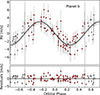 |
Fig. A.1. Phase-folded RV curve of TOI-1710 b. The grey-shaded area shows the ±1σ uncertainties of the model, while the residuals are shown in the bottom panel. The fitted stellar activity and polynomial function are subtracted from the data points. |
First of all, we carefully considered the influence of stellar contamination from neighbouring stars, and verified stellar dilution by computing a dilution factor – the total flux from contaminants falling into the photometric aperture divided by the flux contribution from the target star. We performed the calculation following Mantovan et al. (2022) and imposed a Gaussian prior in the modelling described as follows.
In particular, we simultaneously modelled all TESS-corrected light curves, the off-transit RV, bisector span (BIS), and full width at half-maximum (FWHM) series, and the in-transit RV anomaly. This allowed us to model the planetary transits, the Keplerian signal and orbital obliquity, and the stellar activity using Gaussian processes (GPs, Rajpaul et al. 2015, and references therein). We used BATMAN (Kreidberg 2015) to model the planetary transits. We fitted the following parameters: central time of transit (T0, b), orbital period (Pb), planet to star radius ratio (Rp/R★), impact parameter (b), RV semi-amplitude (Kb), and sky-projected obliquity (λ). Additionally, we calculated the eccentricity (e) and argument of pericentre (ω), by fitting  and
and  (Eastman et al. 2013). We imposed Gaussian priors on the host star density (ρ★) and the projected rotational velocity (v sin i★), while leaving the stellar rotation period (Prot, see below) free to vary. In particular, we treated the stellar equatorial velocity (veq, obtained from the stellar radius R★ and Prot) and inclination (i★) as independent variables. Thus, we are not subject to the bias described in Masuda & Winn (2020). The v sin i★ is a derived parameter; specifically, it is calculated from veq and i★ parameters at each step, and then compared with the given prior. We treated the stellar limb darkening (LD) contribution by estimating u1 and u2 using PyLDTk2 (Husser et al. 2013; Parviainen & Aigrain 2015) and assuming a boxcar filter as the passband in the HARPS-N spectral range and adding 0.1 in quadrature to their Gaussian errors to account for unknown model systematics. We also modelled and fit the effect of stellar convective blueshift (CB) on the in-transit RV curve (e.g. Cegla et al. 2016) using a linear law as a function of limb angle. Short-term stellar activity was included in the model by a jitter term added in quadrature to the RV and photometry errors.
Priors on stellar parameters (including limb-darkening coefficients) are based on posterior distributions from independent analyses, i.e. using data not involved in the fit, as described in Appendix B and Table H.1. Parameters that cannot be measured directly from the RM effect, such as the stellar radius or the stellar inclination, are included in the fit so that they can be combined with other parameters constrained by the RV and photometry (such as the stellar rotation period) and produce self-consistent derived parameters, such as the projected equatorial velocity, for the RM modelling. We emphasise that we checked the robustness of our results by conducting a second analysis without imposing any prior information on vsini (leaving it free to vary). We obtained an almost identical posterior distribution, meaning that the chosen prior was not strongly informative. For all parameters, we employed uninformative boundaries based on physically realistic limits for a star of this spectral type. Specifically for the stellar rotation period, we kept this range wide to explore the parameter space, specifically to test the possible 11-day period solution. For some parameters, we restricted the parameter space while keeping it uninformative to reduce the convergence time. When boundaries are not specified in the table, we kept the default range (conservatively extremely wide) provided by PyORBIT.
We modelled stellar activity in the RV, BIS, and FWHM series using a multidimensional GP, while we used a unidimensional one for the TESS photometric time series. We used an exponential-sine periodic (ESP) kernel as defined in Delisle et al. (2020, 2022) for the multidimensional GP, and a rotation kernel as defined in Foreman-Mackey et al. (2017), Foreman-Mackey (2018). As part of this modelling, we set the rotation period (Prot) as a unique parameter that is shared between the unidimensional GP, the multidimensional GP and the RM modelling. The rest of the GP hyperparameters, such as the characteristic decay timescale (Pdec) and the coherence scale (ωcs), are independent between the photometric and spectroscopic datasets. Finally, we included a third degree polynomial function to model a long-term sinusoidal-like trend present in the spectroscopic time series. This function has coefficients shared among all datasets and a multiplication factor associated with each time series.
We performed a global optimisation of the parameters by running PyDE (Storn & Price 1997; Parviainen 2016) for 100 000 generations and a Bayesian analysis of the RM signal in the RV time series using EMCEE Foreman-Mackey et al. (2013) for 200 000 steps. This choice was motivated by the fact that MCMC samplers allow the specification of a prior on derived parameters, as in the case of v sin i★, which is not possible in the case of nested sampling algorithms. We used 4 × ndim walkers, with ndim the model dimensionality, and discarded the first 50 000 steps (burn-in). We applied a thinning factor of 100 to mitigate the effect of chain autocorrelation.
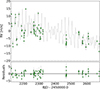 |
Fig. A.2. Modelling of HARPS-N RV time series. Top: RV time series with superimposed full Keplerian + stellar activity + third polynomial function model. Bottom: Residuals of the fit. |
Appendix B: Stellar rotation period refinement
To accurately translate the sky-projected obliquity (λ) into the true 3D orbital obliquity (ψ), we need a reliable stellar rotation period. We estimated this in our fully Bayesian analysis by leaving it free to vary and modelling the activity in our TESS-corrected light curves (which preserve stellar variability), RV, BIS, and FWHM series. This yielded a stellar rotation period Prot = 21.5 ± 0.2 days, which is compatible with that found in K22 and Orell-Miquel et al. (2024). To support our finding, we used the generalised Lomb-Scargle algorithm (Zechmeister & Kürster 2009) to examine the periodogram of the two spectroscopic activity indicators we used (BIS, FWHM) and the RVs. The periodogram of the BIS shows a dominant peak close to 11 days, while the other two close to 21 days. Most TESS sectors also show the highest peak around 10-11 days, with occasional signals close to 17 days. However, sector 79 agrees with previous works, showing the dominant peak at 21 days (Fig. B.1). This stellar variability cannot be physically explained by a faster rotation with a periodicity of half that of the 21-day. Instead, it is possible to observe a shorter period in other light curves if there are two similarly sized spots in opposite hemispheres.
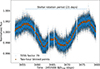 |
Fig. B.1. Photometric time series of TESS sector 79. The 21-day stellar modulation can undoubtedly be seen. |
Given these considerations, we adopt as the most reliable Prot that obtained from our full analysis (see Table H.1), interpreting the 11-day signal as the first harmonic of the stellar rotation. This interpretation is further supported by multiple diagnostics, including the stellar kinematic properties and lithium content, as detailed in the following section.
Appendix C: Independent stellar age diagnostics
First of all, a rotational period of 11 days would imply a gyrochronological age of about 900 Myr, according to the calibration in Mamajek & Hillenbrand (2008). However, the kinematic properties of the star disfavour such a moderately young age. In fact, the space velocities, derived following Johnson & Soderblom (1987), are U = 44.79 ± 0.14 km s−1, V = −20.17 ± 0.12 km s−1, and W = 8.87 ± 0.09 km s−1. These values are well outside the kinematic space in which nearby young (≤ 1 Gyr) stars are confined (Montes et al. 2001). The probability distribution function of the age, evaluated on the basis of the stellar kinematics according to the method in Almeida-Fernandes & Rocha-Pinto (2018), has a maximum at about 4.6 Gyr and gives an estimated kinematic age of 5.2 ± 3 Gyr, thus supporting the results based on Montes et al. (2001). A similar discrepancy would arise for the mean chromospheric activity level log R′HK ≈ −4.78 (König et al. 2022; Orell-Miquel et al. 2024). This differs greatly from what would be expected for a period of 11 days and an age of about 900 Myr (about −4.4 for such G dwarf stars). Conversely, the gyrochronological age resulting from the adopted rotation period, i.e. about 3 Gyr, is instead fully consistent with the age derived from the chromospheric activity and stellar kinematics.
The co-added HARPS-N spectrum of the target show the lithium line at ∼6707.8 Å with a mean equivalent width EWLi = 5.7 ± 0.5 mÅ. This corresponds to a lithium abundance log n(Li) = 1.20 ± 0.05 dex, corrected for non-Local thermal equilibrium effects (Lind et al. 2009) following the spectral synthesis method detailed in Biazzo et al. (2022). Based on the effective temperature reported in K22, the methodology described in Jeffries et al. (2023) and the derived EWLi, we estimate a lower age limit of > 1.3 Gyr for the target. Conversely, its lithium abundance, when placed in a log n(Li)-Teff diagram, is compatible with the lower envelope of M67 members, which implies an upper age limit of < 4.5 Gyr (Sestito & Randich 2005). This result further supports the 21.5-day rotation period, as a half-periodicity would imply an age younger than the lower limit of 1.3 Gyr. It is worth noting that our results agree well with previous age estimates for this system, consistently indicating an age greater than 1.3 Gyr.
To support our findings, we have also computed Prot adopting the equations reported in Noyes et al. (1984). Assuming log R′HK = −4.78 ± 0.03 2022AA...666A.183K and B − V = 0.66 ± 0.03 (Høg et al. 2000), we found the theoretically derived convective overturn time to be τc = 12.6 ± 1.7 d, and Prot = 20.3 ± 3.0 d, in agreement with the value reported in Table H.1.
Appendix D: The inflated nature of TOI-1710 b
The inflated nature of TOI-1710 b, coupled with its low incident flux and late stellar age (see sect. C), suggests it may have resisted standard interior cooling. We propose that tidal heating, produced during the final stages of HEM, may have served as a later energy source (see also Ginzburg & Sari 2017). In line with thermal evolution models by Lopez & Fortney (2014) and previous studies on similarly inflated planets orbiting old stars (Cochran et al. 2011), the inflation of TOI-1710 b may also be attributed to a low mass fraction of heavy elements and a large mass fraction of H-He gas. This would make it more likely to host an extended atmosphere despite its proximity to the star.
The HEM process requires a remarkable decrease of the mechanical energy of the initial planetary orbit that is produced by tidal dissipation inside the planet (e.g. Dawson & Johnson 2018). Specifically, the energy decrease, starting from an initial orbit with a semimajor axis much larger than the present value, is given by Ediss = (1/2)GMsMp/a, where G is the gravitation constant, Ms the mass of the star, Mp the mass of the planet, and a the present orbit semimajor axis. The system parameters give Ediss ∼ 2 × 1035 J. The total duration of the HEM process and, therefore, of the dissipation of such a large amount of energy, can be comparable with the age of the system. Assuming, for example, a duration of 1.0 Gyr, we get an average dissipated power of ∼7 × 10¹⁸ W. Even assuming that all that power is used to evaporate an H/He envelope having the mass of 1% of that of the planet, the lifetime of the envelope is of the order of ∼1.5 Gyr, that is, comparable with the age of the star. Nevertheless, a remarkable fraction of the tidal energy should go into radiation from the planetary atmosphere, thus substantially increasing the evaporation timescale of the envelope. On the other hand, such an internal tidal heating, extended over a timescale comparable with the age of the system, can effectively oppose the contraction of the planet associated with its cooling after formation (e.g. Lopez & Fortney 2014), thus keeping its structure inflated.
At the same time, the HEM scenario that we propose offers a plausible explanation for TOI-1710 b to have escaped atmospheric erosion. Planets undergoing disc-migration typically arrive in close-in orbits within 10 Myr, exposing them to the full, constant XUV irradiation of the star in its active phase. In contrast, planets undergoing late HEM may escape this phase (e.g. Bourrier et al. 2018; Attia et al. 2021). Although the XUV flux at pericentre is significantly higher than during disc-migration (potentially four times that of the final circular orbit), the planet spends most of its time at apocentre, safe from intense XUV flux irradiation. A planet on a highly eccentric orbit (e≈ 0.8) spends only about 1.2% of its orbital period within ± 30 deg of pericentre (5% when e≈ 0.5). This reduced exposure likely enabled TOI-1710 b to survive as a gas-rich world. Another possible explanation for the photo-evaporation resistance and inflation of TOI-1710 b is in the metal-rich nature of TOI-1710 (see Tab. H.2). This possible correlation was first noted by Wilson et al. (2022), which postulated that planets orbiting metal-rich stars have metal-rich atmospheres with reduced photo-evaporation.
Appendix E: Search for planetary companions
We tested for the presence of additional planetary companions by performing the same Bayesian analysis detailed in Sect. A, including one or two additional Keplerian signals. Specifically, we imposed wide uniform priors on their orbital periods (0 – 2000 days), eccentricities and RV semi-amplitudes (0.01 – 50 m s−1). This further test was performed due to the large obliquity found and its dynamical implications, which are discussed in the following section. Moreover, the analysis was motivated by the relatively large value of the uncorrelated RV jitter (1.4 m s−1).
The two-planet solution gives a similar jitter value and finds a candidate signal at approximately 1650 days with a high eccentricity (> 0.8). Instead, the three-planet model results in a slightly lower jitter of 1.3 m s−1 and suggests two different candidate signals with periods of about 1480 and 105 days, both detected at 3σ. The period of the wide orbit candidate in this model is inconsistent with the one found in the two-planet solution, which suggests that the corresponding RV signal is more likely to be of stellar origin, and that it could not be perfectly modelled with the polynomial trend. We repeated these analyses with the third degree polynomial function removed. As before, the long-period candidate changes its periodicity in the two- and three-planet solutions. However, the period and amplitude of the third signal remained compatible.
To compare the one-, two- and three-planet solutions, we used the Bayesian information criterion (BIC; Schwarz 1978). We performed the comparison separately for the models with and without the polynomial function included. As shown in Table E.1, the one-planet solution is strongly preferred in both cases. It is worth noting that the Keplerian and obliquity solutions for planet b show little variation (less than one sigma) across the tested models, further strengthening the results (see Appendix. A) and conclusions of this work.
Bayesian information criterion values for the different models tested.
Appendix F: Detection completeness map
To quantify our sensitivity to additional companions, we performed an injection-recovery analysis, based on the HARPS-N RVs, following the same approach used in Naponiello et al. (2025). We explored a logarithmic grid in planetary minimum mass, ranging from 10−1 MJup to 20 MJup, and semi-major axis (a), from 10−2 to 10 au. For each grid cell, we generated 200 synthetic planetary systems. The orbital period was derived from a, while the time of conjunction and argument of periastron were drawn from uniform distributions. The inclination was sampled from a sinusoidal distribution (i.e. uniform in cos i), and the eccentricity was drawn from a Beta distribution following Kipping (2013), representative of the observed exoplanet population.
For each simulated planet, we generated synthetic RV time series at the actual observing epochs and added Gaussian noise scaled to the instrumental jitter reported in Table H.3. We then compared three models: (i) a constant model, (ii) a polynomial trend (linear or quadratic) to account for long-period variability, and (iii) a full Keplerian model. Model selection was performed using the BIC, defined as BIC = χ2 + klnNobs, where k is the number of free parameters and Nobs the number of measurements. A planet was considered detected if the Keplerian model was preferred over the simpler models with ΔBIC > 10 (Kass & Raftery 1995). In addition, signals producing significant linear or quadratic trends were flagged as detected when the polynomial model was favoured over the constant one. The completeness map (Fig. F.1) reports, for each grid cell, the fraction of recovered planets, defined as Ndet/Nsim. With the current HARPS-N dataset, our sensitivity allows us to robustly detect Jupiter-mass companions out to approximately ∼4 au, while lower-mass planets remain detectable only at shorter orbital separations.
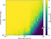 |
Fig. F.1. Detection completeness map for TOI-1710 in the mass versus semi-major axis plane, based on the RV injection-recovery analysis. The colour scale represents the fraction of simulated planetary companions recovered in each grid cell. For reference, the locations of Jupiter and Saturn are shown as icons. |
Appendix G: Probing photo-evaporation via HeI triplet and Hα
We conducted a multi-band transmission spectroscopy analysis to better understand the atmospheric properties of TOI-1710 b. In particular, we investigated two key tracers of extended and possibly escaping atmospheres: the HeI triplet at 1083.3 nm (GIANO-B data) and the Hα line (HARPS-N data, D’Arpa et al. 2024). We carried out HeI and Hα transmission spectroscopy by comparing in- and out-of-transit spectra, following the methodology described in Guilluy et al. (2024) and D’Arpa et al. (2024).
We did not detect any clear absorption features at the positions of the HeI triplet or the Hα line. Following the method of Guilluy et al. (2024), we report 1σ upper limits on the excess absorption at the expected line positions of 0.58% for HeI and 0.29% for Hα, corresponding to effective planetary radii of 1.8 Rb and 1.5 Rb, respectively. The non-detection of HeI and Hα for TOI-1710 b is not surprising. The planet’s relatively low equilibrium temperature (Teq ≈ 670 K), combined with its long orbital period, may reduce the effects of stellar irradiation, inhibiting the population of the n = 2 level from which the Hα transition originates. The same applies to HeI, where the planetary distance from the star may reduce the XUV flux, disfavouring the mechanisms of ionisation and recombination that leads to formation of the metastable HeI triplet.
Appendix H: Extra figures and tables
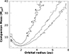 |
Fig. H.1. Astrometric Gaia DR3 sensitivity map for companions. The dashed, dotted and long-dashed lines correspond to isoprobability curves for 80, 90 and 99% probability of a companion with given properties producing RUWE > 0.94. |
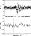 |
Fig. H.2. Final transmission spectrum around the Hα (top) and HeI (bottom) evaporation diagnostics. In the right panel, vertical black dotted lines indicate the position of the HeI triplet. |
Priors and outcomes of RM modelling.
Literature stellar parameters.
Priors and outcomes of full modelling.
All Tables
All Figures
|
Fig. 1. Rossiter-McLaughlin fit to the in-transit RV of TOI-1710 b. Top: Best-fit (line) over the RVs data, corrected for the Keplerian RV curve and systemic RV. Bottom: Residuals of the fit. |
| In the text | |
|
Fig. 2. True obliquity of known exoplanets vs. host star effective temperature. TOI-1710 b is indicated by a star. The a/R★ is colour-coded. The shaded region denotes Teff > 6250 K. Data: TEPCat and the NASA Exoplanet Archive as of February 2026. |
| In the text | |
|
Fig. 3. True obliquity of super-Neptunes vs. orbital period. Planetary densities are differentiated by colour and eccentricities by size. The shaded areas separate the desert, ridge, and savanna. |
| In the text | |
|
Fig. A.1. Phase-folded RV curve of TOI-1710 b. The grey-shaded area shows the ±1σ uncertainties of the model, while the residuals are shown in the bottom panel. The fitted stellar activity and polynomial function are subtracted from the data points. |
| In the text | |
|
Fig. A.2. Modelling of HARPS-N RV time series. Top: RV time series with superimposed full Keplerian + stellar activity + third polynomial function model. Bottom: Residuals of the fit. |
| In the text | |
|
Fig. B.1. Photometric time series of TESS sector 79. The 21-day stellar modulation can undoubtedly be seen. |
| In the text | |
|
Fig. F.1. Detection completeness map for TOI-1710 in the mass versus semi-major axis plane, based on the RV injection-recovery analysis. The colour scale represents the fraction of simulated planetary companions recovered in each grid cell. For reference, the locations of Jupiter and Saturn are shown as icons. |
| In the text | |
|
Fig. H.1. Astrometric Gaia DR3 sensitivity map for companions. The dashed, dotted and long-dashed lines correspond to isoprobability curves for 80, 90 and 99% probability of a companion with given properties producing RUWE > 0.94. |
| In the text | |
|
Fig. H.2. Final transmission spectrum around the Hα (top) and HeI (bottom) evaporation diagnostics. In the right panel, vertical black dotted lines indicate the position of the HeI triplet. |
| In the text | |
Current usage metrics show cumulative count of Article Views (full-text article views including HTML views, PDF and ePub downloads, according to the available data) and Abstracts Views on Vision4Press platform.
Data correspond to usage on the plateform after 2015. The current usage metrics is available 48-96 hours after online publication and is updated daily on week days.
Initial download of the metrics may take a while.