


| Issue |
A&A
Volume 711, July 2026
|
|
|---|---|---|
| Article Number | A277 | |
| Number of page(s) | 9 | |
| Section | Planets, planetary systems, and small bodies | |
| DOI | https://doi.org/10.1051/0004-6361/202659619 | |
| Published online | 21 July 2026 | |
Influence of topography on the atmospheric thermal tides and rotational evolution of Venus
1
Nantes Université, Univ Angers, Le Mans Université, CNRS, Laboratoire de Planétologie et Géosciences,
LPG UMR 6112,
44000
Nantes,
France
2
LIRA, Observatoire de Paris, Université PSL, Sorbonne Université, Université Paris Cité, CY Cergy Paris Université, CNRS,
Meudon,
France
3
Laboratoire de Météorologie Dynamique, Sorbonne Université, ENS, PSL Research University, École Polytechnique, Institut Polytechnique de Paris, CNRS,
Paris,
France
★ Corresponding author: This email address is being protected from spambots. You need JavaScript enabled to view it.
Received:
26
February
2026
Accepted:
10
June
2026
Abstract
Context. Venus’ rotation is the slowest of all the planets in the Solar System and is in the retrograde direction. Such a rotational state results directly from several tidal effects that impact both the atmosphere and the solid part of the planet. To fully characterize the rotational dynamics and evolution of Venus, it is therefore mandatory to have a comprehensive understanding of the various factors that influence the different tidal effects and in particular the atmospheric thermal tides.
Aims. In this context, this work investigates how the distribution of the topography, which likely changed during Venus’ history through resurfacing events or true polar wander (TPW), affect the atmospheric thermal tides and, consequently, the rotational state of the planet. Moreover, we examine how the presence of topography affects the dependence of the atmospheric thermal torque on the rotation period and how it may have influenced the global evolution of the rotation.
Methods. Using the Venus Planetary Climate Model (V-PCM), we first focused on characterizing the influence of the topography on atmospheric thermal tides. For that purpose, we performed a series of global atmospheric dynamics simulations exploring various configurations of the topography and computed the atmospheric thermal torques from the surface pressure anomalies. Second, we updated an empirical law that links the atmospheric thermal torque to the forcing frequency by evaluating the strength of the atmospheric tides at different rotation periods using V-PCM simulations.
Results. Our results first highlight the link between topography and thermal tides, showing that the variations in the atmospheric thermal torque over a solar day are mainly controlled by the large-scale near-equatorial topography. Moreover, we show that changes in the topography not only introduce strong diurnal variations in the torque but also change its daily average value, and therefore impact the whole rotational evolution of the planet.
Conclusions. This study highlights that the rotational state and evolution of Venus, as well as other planets and exoplanets, therefore depend on the variations in the topography and that modeling it without including this topographic effect can introduce significant uncertainties.
Key words: planets and satellites: atmospheres / planets and satellites: dynamical evolution and stability / planets and satellites: terrestrial planets
© The Authors 2026
 Open Access article, published by EDP Sciences, under the terms of the Creative Commons Attribution License (https://creativecommons.org/licenses/by/4.0), which permits unrestricted use, distribution, and reproduction in any medium, provided the original work is properly cited.
This article is published in open access under the Subscribe to Open model. This email address is being protected from spambots. You need JavaScript enabled to view it. to support open access publication.
1 Introduction
Venus exhibits a unique rotational state in the Solar System, characterized by a very slow asynchronous retrograde rotation with a period of 243 Earth days (Smith 1963; Carpenter 1964; Goldstein 1964; Margot et al. 2021). This present-day rotation and its evolution through time mainly result from the interaction between several tidal processes, in particular, the gravitational solid tides, the atmospheric thermal tides, and other secondary effects (Gold & Soter 1969; Goldreich & Peale 1970; Correia & Laskar 2001, 2003; Revol et al. 2023; Musseau et al. 2024).
Gravitational solid tides arise on a planet from the gradient of the gravitational potential exerted by a perturbing body, here the Sun. The resulting tidal forces deform the solid body, creating tidal bulges on opposite sides of the planet. The viscoelastic response to the tidal forcing causes a lag in the deformation, shifting the planet’s principal axis away from the direction toward the perturbing body. This deformation generates a gravitational torque that gradually drives the planet’s rotation toward spin-orbit synchronization. On the other hand, atmospheric thermal tides are generated by the redistribution of atmospheric mass due to thermal perturbation. Heating of the day side of the atmosphere by solar insolation induces a strong dichotomy in the temperature distribution. This temperature gradient drives energy transfer toward cooler regions through mass redistribution from the day side to the night side of the planet, resulting in surface pressure variations with higher pressure on the night side due to a positive atmospheric mass anomaly, and lower pressure on the day side. Focusing on degree 2 and order 2 of this deformation, the atmosphere shapes as an ellipsoid with two atmospheric pressure bulges on either side of the planet. The deformation of the atmosphere, delayed in time by thermal inertia, is not instantaneous and creates a lag between the main axis of the atmosphere and the Venus-Sun direction. This lag generates an atmospheric thermal torque due to the gravitational attraction of the Sun that accelerates Venus’ rotation and tends to drive it out of synchronization (Correia & Laskar 2003). Besides these two primary effects, the rotational state of Venus is also influenced by the gravitational torque upon pressure bulge, which represents the deformation of the solid body due to the mass of the atmospheric pressure bulge, and by the pressure torque upon tidal bulge, which reflects the gravitational coupling between the gravitational bulge and the pressure bulge (Correia & Laskar 2003; Musseau et al. 2024). While the effects of the solid part are expected to have been relatively stable over the last billion years, as they are primarily controlled by the viscosity profile, which evolves on long timescales (Gillmann & Tackley 2014), the effects of the atmosphere could have changed significantly, thereby creating variations in Venusian rotation. Understanding these variations requires a detailed characterization of the physical mechanisms that control the amplitude of atmospheric thermal tides, as has been done for the effects of the mean atmospheric mass, the rotation period, the stellar luminosity, and the atmospheric composition (Leconte et al. 2015; Auclair-Desrotour et al. 2017; Revol et al. 2023; Salazar & Wordsworth 2024).
Topography is known to play a crucial role in modulating surface pressures and temperatures, as well as influencing atmospheric circulation. For instance, it affects the intensity of zonal winds (Bertaux et al. 2016) and generates atmospheric gravity waves, commonly referred to as mountain waves (Fukuhara et al. 2017; Navarro et al. 2018; Lefèvre et al. 2020). Topography is therefore also expected to influence the amplitude and temporal variability of atmospheric thermal tides. This aspect is particularly relevant for studies of the evolution of Venus’ rotation because the topography may have changed significantly over a short geological timescale (<1 Gyr). Indeed, the low number of meteoritic impacts indicates that Venus’ surface is relatively young compared to other planetary surfaces, most likely due to local or global resurfacing events that would have significantly reshaped the topography through the formation of new volcanic structures (Strom et al. 1994; Herrick et al. 1997; Phillips et al. 1992; Herrick et al. 2023). In addition to resurfacing, true polar wander (TPW) could have strongly affected the orientation and global distribution of the topography. A TPW is defined as a reorientation of the entire solid body with respect to its rotation axis, driven by internal or surface mass redistribution and associated changes in the planet’s inertia axis (e.g., Matsuyama et al. 2014; Leconte 2018). Although TPW does not modify the topography itself, it changes the repartition and orientation of the topographic features at the surface. On Earth, modern TPW (20th century) has been inferred from astronomical and geodetic measurements to occur at rates of about 1° Myr−1, a behavior mainly attributed to glacial isostatic adjustment and mantle convection dynamics (e.g., Wu & Peltier 1984; Argus & Gross 2004; Mitrovica et al. 2005; Ghelichkhan et al. 2025). Such a TPW rate could have produced a reorientation of about 30° within 25 Myr (Steinberger 2008; Fu & Kent 2018), but may have been lower earlier in geological history (e.g., Greff-Lefftz 2004). On Venus, a TPW may also have modified the planet’s orientation as it did on Earth. Even if the main mechanism driving TPW on Earth (glacial isostatic adjustment) probably did not occur on Venus, TPW caused by mantle dynamics could still play a significant role in Venus’ orientation because of its reduced oblateness, a consequence of its slow rotation (Hu et al. 2017; Patočka 2021; Patočka et al. 2025). Even though the existence of a TWP on Venus remained theoretical for a long time, recent studies measured that Venus may have experienced TPW at rates comparable to Earth’s one, based on the orientation of old wind-blown ejecta deposits that could have recorded a geologically recent TPW (Austin et al. 2025). Such a rate would have significantly reorganized the distribution of the topography over time and, if atmospheric tides are indeed sensitive to the topography, could have modified the atmospheric thermal torque and the rotational evolution of Venus.
To address this question, we conducted a series of Venusian atmospheric dynamic simulations for a variety of topographic configurations presented in the first section. The resulting pressure anomaly and atmospheric thermal torque are then analyzed in Sect. 3 to highlight the effect of the topography on the amplitude and variability of atmospheric thermal tides and to quantify its effect on the recent evolution of Venus’ rotation. Finally, the dependence of atmospheric thermal tides on the forcing frequency is studied, taking into account this new effect of the topography.
2 Methods
The influence of topography on atmospheric thermal tides and the rotation period was analyzed from numerical simulations performed using a planetary climate model with several topographic configurations described in detail below. The surface pressure fields obtained from these simulations were then used to compute the surface pressure anomaly, the complex quadrupolar pressure anomaly coefficient, ![Mathematical equation: $\[\tilde{p}_{2}^{2}\]$](/articles/aa/full_html/2026/07/aa59619-26/aa59619-26-eq1.png) , and the associated atmospheric thermal torque. The full methodology used to derive the atmospheric thermal torque from surface pressure is detailed in Sect. 2 of Musseau et al. (2024) and summarized hereafter.
, and the associated atmospheric thermal torque. The full methodology used to derive the atmospheric thermal torque from surface pressure is detailed in Sect. 2 of Musseau et al. (2024) and summarized hereafter.
2.1 Synthetic topographies
Two reference topographies were considered as a baseline for comparison with other configurations. The first one corresponds to present-day Venusian topography, while the second one is a case with no topography, i.e., where the surface altitude is set to 0 m everywhere. This second case was considered to obtain pure atmospheric thermal tides features, unaffected by any topographic effect, and to compare it with previous studies (Leconte et al. 2015).
Because the past topography of Venus is unknown, we focused our study on the effect of a TPW acting on the present-day topography. In this framework, the current topography is preserved, but its position relative to the rotation axis is modified. This approach allowed us to isolate the effect of large-scale reorientation without introducing speculative topographies. All topographies were constructed from high-resolution topography (4096 × 8192) derived from Magellan data. The reorientation of the topography was then performed using the SHTools Python package (Wieczorek & Meschede 2018, version 4.13). The topography was first expanded into spherical harmonic coefficients and then reoriented using the SHTools rotate function, which bases the rotation on the three Euler angles. To explore different topographic configurations, we performed two subsequent rotations: one along the vertical axis, Z, and one along the horizontal axis, Y. These rotations can be described with two different angles, αlon and αlat, respectively (see the left panel of Fig. 1). The first, αlon, specifies the position of the 0° longitude relative to its current position. The second, αlat, defines the latitude of the current geographic pole with respect to the rotational axis unchanged along the Z axis, i.e., the amplitude of the TPW. To maximize the diversity of topographic configurations, we first rotated the topography with the αlon angle, shifting the topographic features along the longitudes. Then, the topography was rotated along the 180° longitude with the αlat angle, which moves the topographic features toward or away from the poles. The latitudinal angle, αlat, was varied between 0° and 90°, while the longitudinal angle, αlon, was explored from 0° to 330°. In this referential, the current topography corresponds to αlat=0° and αlon=0°. After the rotation, the high-resolution topography was reconstructed from the modified spherical harmonic coefficients. Figure 1 illustrates how the angles αlat and αlon operate and displays examples of the topographies obtained by applying these rotations, compared to the current topography. A rotation using only the angle αlon does not change the overall distribution of the topography, since it only makes a rotation around the rotation axis. However, the combined action of both angles can produce a large variety of topographic distributions. The simulations corresponding to these topographies are hereafter named according to the rotation, following the format H–αlat–αlon.
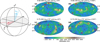 |
Fig. 1 Creation of synthetic topography fields using rotations of Venus’ current topography. Left: illustration of the angles, αlat and αlon, that define the reorientation applied on the topography. The angle αlat defines the latitude of the geographic pole with respect to the rotational axis. The angle αlon defines the position of the 0° longitude relative to its present-day position. The present-day topography is therefore given by αlat = 0° and αlon = 0°. Right: topographic maps for several configurations. (a) αlat = 0° and αlon = 0° (current topography). (b) αlat = 0° and αlon = 150°. (c) αlat = 75° and αlon = 0°. (d) αlat = 75° and αlon = 150°. The transition from (a) to (b) correspond to a variation in αlon resulting in a longitudinal rotation of the topography. The transition from (a) to (c) correspond to a variation in the αlat angle resulting in a latitudinal rotation. The transition from (a) to (d) represents a combined variation in both angles. Letter A–E indicate the locations of the principal provinces of Venus, with A=A phrodite Terra, B=Ishtar Terra, C=Alta Regio, D=Guinevere Planitia, and E=Lavinia Planitia. |
2.2 Simulations of atmospheric dynamic
The surface pressure field was obtained from 3D atmospheric dynamic simulations made with the latest version of the LMDZ Venus PCM (V-PCM, revision no3853, Lebonnois et al. 2010, 2016; Martinez et al. 2023). The initial state of the simulations is taken from Lai et al. (2024) and corresponds to the final time-step of a 40 Venusian days simulation (1 Venusian day = 116.75 earth days) that reproduces the Venus Climate Database (VCD) for mean EUV conditions and standard cloud albedo. Sensitivity analyzes conducted using the VCD indicate that adopting alternative EUV conditions (solar maximum and minimum activity), as well as different albedo, does not significantly affect the results, with current torque estimates varying by only about 1%. This initial state is modified with the topographic configurations presented in the previous section and is run for at least 20 Venusian days, which is sufficient for the model to reach convergence, with a 96 × 96 spatial resolution and 50 vertical levels.
2.3 Computing the surface pressure anomaly coefficient, ![Mathematical equation: $\[\tilde{p}_{2}^{2}\]$](/articles/aa/full_html/2026/07/aa59619-26/aa59619-26-eq2.png)
The surface pressure anomaly coefficient, ![Mathematical equation: $\[\tilde{p}_{2}^{2}\]$](/articles/aa/full_html/2026/07/aa59619-26/aa59619-26-eq3.png) , was then evaluated over a Venusian day using the surface pressure field previously simulated for all the topographic configurations. Following Bills et al. (2020), the surface pressure was decomposed into a constant part and a dynamic part. The constant part was defined as the daily mean surface pressure field, which mainly reflects the influence of the topography on the atmospheric mass distribution. The dynamic part corresponds to the remaining time-varying component of the surface pressure and includes only the dynamic processes that have a zero mean over a complete Venusian day. This part is dominated by the effect of the atmospheric thermal tides displaying a negative anomaly following the subsolar point with a lag. By expanding the dynamic part in spherical harmonics, the complex coefficient of the pressure anomaly field,
, was then evaluated over a Venusian day using the surface pressure field previously simulated for all the topographic configurations. Following Bills et al. (2020), the surface pressure was decomposed into a constant part and a dynamic part. The constant part was defined as the daily mean surface pressure field, which mainly reflects the influence of the topography on the atmospheric mass distribution. The dynamic part corresponds to the remaining time-varying component of the surface pressure and includes only the dynamic processes that have a zero mean over a complete Venusian day. This part is dominated by the effect of the atmospheric thermal tides displaying a negative anomaly following the subsolar point with a lag. By expanding the dynamic part in spherical harmonics, the complex coefficient of the pressure anomaly field, ![Mathematical equation: $\[\tilde{p}_{2}^{2}\]$](/articles/aa/full_html/2026/07/aa59619-26/aa59619-26-eq4.png) , was obtained at degree and order 2.
, was obtained at degree and order 2.
2.4 Computing atmospheric thermal torque, Γth
The influence of atmospheric tides on the rotational state of Venus for all atmospheric simulations can be expressed through the atmospheric thermal torque, Γth. Following Leconte et al. (2015), Γth is defined from the gravitational potential of the deformed atmosphere and can be related to the surface pressure anomaly field. Assuming hydrostatic equilibrium of the atmosphere and a zero obliquity of the rotation axis, which is close to Venus’ case (Margot et al. 2021, and references therein), the atmospheric torque can be defined with
![Mathematical equation: $\[\Gamma_{t h}=-\frac{G M_s R_p}{g} \sum_{\ell=2}^{\infty} \frac{4 \pi}{2 \ell+1}\left(\frac{R_p}{a}\right)^{\ell+1} \sum_{m=-\ell}^{\ell} \mathrm{i} m \tilde{p}_{\ell}^m Y_{\ell}^m\left(\theta_s=\frac{\pi}{2}, \Phi_s\right),\]$](/articles/aa/full_html/2026/07/aa59619-26/aa59619-26-eq5.png) (1)
(1)
where G, Ms, Rp, g, and a are the gravitational constant, the solar mass, Venus’ radius, the gravitational acceleration, and the semi-major axis of the orbit (Leconte et al. 2015; Musseau et al. 2024). The term ![Mathematical equation: $\[\tilde{p}_{\ell}^{m}\]$](/articles/aa/full_html/2026/07/aa59619-26/aa59619-26-eq6.png) corresponds to the complex coefficients of the spherical harmonic expansion of the surface pressure anomaly field for all degrees, ℓ, and orders, m. We employ in this study the spherical harmonics normalization described in Musseau et al. (2024). Because degrees 0 and 1 correspond, respectively, to a constant pressure term and a shift of the center-of-mass position, they do not contribute to the torque. Moreover, degrees higher than 2 are negligible compared to degree 2 because the factor (Rp/a)ℓ+1 becomes much lower than 1. Keeping only the degree 2 term, Γth becomes
corresponds to the complex coefficients of the spherical harmonic expansion of the surface pressure anomaly field for all degrees, ℓ, and orders, m. We employ in this study the spherical harmonics normalization described in Musseau et al. (2024). Because degrees 0 and 1 correspond, respectively, to a constant pressure term and a shift of the center-of-mass position, they do not contribute to the torque. Moreover, degrees higher than 2 are negligible compared to degree 2 because the factor (Rp/a)ℓ+1 becomes much lower than 1. Keeping only the degree 2 term, Γth becomes
![Mathematical equation: $\[\Gamma_{t h}=\frac{3}{2} \frac{3 M_s R_p^3}{5 \bar{\rho} a^3} \sqrt{\frac{10}{3 \pi}} \Im \mathrm{m}(\tilde{p}_2^2 e^{2 \mathrm{i} \phi_s}),\]$](/articles/aa/full_html/2026/07/aa59619-26/aa59619-26-eq7.png) (2)
(2)
where ![Mathematical equation: $\[\bar{\rho}\]$](/articles/aa/full_html/2026/07/aa59619-26/aa59619-26-eq8.png) is the mean density of the planet and
is the mean density of the planet and ![Mathematical equation: $\[\tilde{p}_{2}^{2}\]$](/articles/aa/full_html/2026/07/aa59619-26/aa59619-26-eq9.png) is the surface pressure anomaly coefficient computed from surface pressure simulations.
is the surface pressure anomaly coefficient computed from surface pressure simulations.
3 Results
3.1 Simulations with and without topography
To quantify how the topography affects the atmospheric thermal torque, Fig. 2 compares the Γth over a Venusian day for the reference simulations with and without topography. The torque estimated by Leconte et al. (2015) is also included for comparison. Figure 2 clearly shows that introducing the topography affects both the amplitude and the daily variations in the torque. For the simulation without topography, the mean torque is larger in amplitude and very stable over time, with fluctuations of less than 27% around the average torque. When topography is included, the torque shows important temporal variability (larger than 115%) with three distinct maxima over the day. The comparison between these two cases therefore indicates a clear influence of the presence of an underlying topography on the atmospheric thermal torque, creating strong modulation of Γth during the day and impacting the average value of the torque. The torque computed by Leconte et al. (2015) from a simulation without topography and using an earlier version of the V-PCM also displays weak temporal variability consistent with our simulation without topography and corroborating the previous conclusion. However, this third case also exhibits a lower mean amplitude compared to our simulation without topography, highlighting a significant effect of the V-PCM version that lies beyond the scope of this study.
3.2 Simulations with synthetic topographies
To better understand the role of topography on the atmospheric thermal torque, Γth, we simulated the atmospheric dynamic for various topographic configurations to determine whether the signature of the topography is identifiable in the surface pressure anomaly field and the resulting atmospheric thermal torque. Comparing the topography with the pressure anomaly fields used in the torque calculation provides a clearer picture of how topography generates variations in atmospheric dynamics and affects the atmospheric thermal tides. Figure 3 presents examples of pressure anomaly fields obtained for three different topographies represented above. These topographies correspond to small (H-15-030) and stronger reorientations (H-75-210 and H-90-000). The spatial variations in the pressure anomaly appear to closely coincide with the underlying topography, particularly with the large scale provinces located at low latitudes. For instance, in all three cases, Aphrodite Terra, characterized by a high altitude, can be identified as a region with a near-zero pressure anomaly. Ishtar Terra, by contrast, does not appear in the pressure anomaly field when it is located at a high latitude (H-15-030 simulation), but becomes clearly visible when the high TPW shifts it toward lower latitudes, as in the H-75-210 simulation. Specifically, highlands systematically exhibit pressure anomalies close to zero. In contrast, lowlands display stronger pressure anomaly amplitudes than their surroundings. This behavior can be directly linked to the air mass column above the topography involved in atmospheric dynamical processes. Indeed, the atmospheric mass is concentrated in the lowest layers of the atmosphere. Therefore, over lowlands, a greater atmospheric mass participates in dynamical processes and thermal tides, leading to higher pressure anomalies. In contrast, over highlands, the atmospheric mass involved is reduced, and the resulting pressure anomalies remain close to zero. Focusing on atmospheric thermal tides, the presence of topography generates large-scale variations in the negative pressure anomaly that follow the subsolar point, amplifying the negative anomaly when located above lowlands and weakening it above highlands. Thus, depending on where the subsolar point is located on the surface, the signature of atmospheric thermal tides in the surface pressure can be more or less pronounced.
If the distribution of the topography over the surface can be directly observed in the pressure anomaly field, the same is true for the signal of the atmospheric thermal torque over a day. To illustrate this effect, Fig. 4 shows the degree 2 and order 2 surface pressure anomaly (represented by the reds and blues contours) at six different times of the day for a simulation using the present-day topography. Since the pressure anomaly is more clearly linked to the large-scale variations of the topography, only the first five spherical harmonic orders of the topography are depicted on the maps by the colored background. The atmospheric thermal torque is represented in the bottom panel as a function of the subsolar point longitude. The six specific times were selected to coincide with local extrema of the Γth profile, i.e., local minima and maxima. The subsolar point longitudes for these times are indicated on the torque signal by the dotted red lines. Tracking the negative pressure anomaly that follows the subsolar point (dotted black line), we find that when the atmospheric torque reaches a minimum, i.e., when the torque is strongly negative, the pressure anomaly is located above lowlands. In contrast, when the pressure anomaly is located over an elevated topography, the atmospheric torque is higher, i.e., closer to zero. For example, when the negative pressure anomaly is above highlands such as Alta Regio (Fig. 4b) or Aphrodite Terra (Fig. 4f), the atmospheric thermal torque reaches values that are lower in amplitude (>−1e16 N m). In contrast, when the negative anomaly is mainly above lowlands such as Guinevere Planitia and Lavinia Planitia (Fig. 4c), the atmospheric thermal torque can reach values that are higher in amplitude (<−3e16 Nm). For their part, intermediate mean elevations provide intermediate torque values (Figs. 4a and 4d). Finally, large scale topographies at high latitudes, such as Ishtar Terra, have no effect on the amplitude of atmospheric thermal tides because the day-night temperature gradient is weaker and the degree 2 of spherical harmonics mainly capture variations at low and mid latitudes. The same behavior is observed for all simulated topographies (see another example in Fig. A.1). This result reinforces the previously identified relationship between the topography and the amplitude of atmospheric thermal tides, indicating that large-scale topographic variations at low latitudes are the main factor controlling the modulation of atmospheric thermal torque during a Venusian day.
 |
Fig. 2 Atmospheric thermal torque over one Venusian day for three simulations. Blue and red lines display the torque for a reference simulation with (H-00-000) and without topography, respectively. The green line corresponds to the torque obtained without topography by Leconte et al. (2015). The daily mean values of these three torques are depicted in dashed lines. |
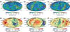 |
Fig. 3 Topographic (panels a–c) and pressure anomaly (panels d–f) maps for three different topographic configurations. (a) and (d): αlat = 15° and αlon = 30° (H-15-030). (b) and (e): αlat = 75° and αlon = 210° (H-75-210).(c) and (f): αlat = 90° and αlon = 0° (H-90-000). The black lines display the topographic contours in all panels, while the thick dotted black line indicates the longitude of the subsolar point. Letter A–E indicate the locations of the principal provinces of Venus, as defined in the caption of Fig. 1. |
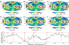 |
Fig. 4 H-00-000 simulation (current topography, αlat =0° and αlon =0°). Top: comparative maps showing the reconstructed topography from the first five spherical harmonic orders of altitude and the quadrupolar pressure anomaly at various times of day. The topography is displayed as the colored background, while the pressure anomaly is indicated by red (positive) and blue (negative) contours. Bottom: atmospheric thermal torque as function of the subsolar point longitude. The dotted red lines indicate the longitude of the subsolar point for the six maps presented in the top panel. Letter A–E indicate the locations of the principal provinces of Venus, as defined in the caption of Fig. 1. |
3.3 Influence of the topography on the rotational evolution
If the presence of the topography introduces strong diurnal variations in the atmospheric thermal torque, it also modifies its average value over a day. Among all the atmospheric simulations performed with several topographic configurations, the daily mean Γth ranges between −1.68 × 10¹⁶ and −1.44× 10¹⁶ N m. Assuming that the current rotation rate results from an equilibrium between atmospheric thermal tides, solid gravitational tides, and other minor tidal effects, a variation in the thermal atmospheric torque of this magnitude should lead to a change in the rotation rate. To quantify this impact, we computed the variation in the rotation period resulting from the change in the atmospheric thermal torque. The new equilibrium rotation period is defined as the rotation period for which the solid gravitational torque, Γg, the gravitational torque upon pressure bulge, Γgp, and the pressure torque upon tidal bulge, Γpg, all dependent on the rotation period, compensate the new Γth. This equilibrium rotation period does not represent the planet’s actual final rotation period but only highlights the influence of the atmospheric thermal tides variations on Venus’ rotational state. Indeed, assessing the real equilibrium rotation period would require considering the feedback loop between tides and rotation, as well as additional effects such as core-mantle friction or planetary perturbations. The equilibrium was determined by computing the tidal and load Love numbers according to the method described in detail in Sect. 2.2 of Musseau et al. (2024) and by calculating the torques, Γg, Γgp, and Γpg. Starting from the current rotation period, we performed an iterative adjustment procedure seeking the rotation period for which the Love number and the associated torques compensate the effect of the atmospheric thermal tides, giving the equilibrium rotation period. For this study, a three-layer viscosity structure (see Fig. 5) explaining the current equilibrium state of Venus (Musseau et al. 2024), as well as density and rheological profiles V5-Th from Dumoulin et al. (2017), are considered. This internal structure is not unique, as a large range of viscosity and density profiles can reproduce the same equilibrium state. However, the choice of internal profile does not significantly affect the results presented here, as the observed variations are driven by changes in the atmospheric tides rather than by the internal contributions.
Figure 5 presents the equilibrium rotation periods as a function of the different atmospheric thermal torques obtained for all the investigated topographic configurations. This figure illustrates that the modification of the topographic distribution, and thus the alteration of the atmospheric thermal tides, can result in a significant change in the equilibrium rotation period, leading to values ranging from −277 days to −110 days. Variations in the equilibrium rotation of this magnitude would lead to a significant acceleration or slowdown of the rotation, influencing the global rotational evolution of Venus. As a comparison, completely removing the topography would lead to a stronger effect, with an equilibrium rotation period of about −307 days, demonstrating how much the topography can control the rotational state of the planet.
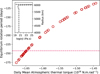 |
Fig. 5 Equilibrium rotation period as function of the atmospheric thermal torque computed for all the investigated topographic configurations. The current rotation period is indicated by the dotted pink line. The three-layer viscosity profile (composed by a crust, an upper mantle, and a 10 times more viscous lower mantle above a liquid core) used to compute the equilibrium rotation period is also represented in the upper right corner. |
3.4 Influence of the rotation period on the rotational evolution
As shown before, any change in topography affects the amplitude of thermal torque, and thus plays a key role in the long-term evolution of Venus’ rotation. In particular, any change in the rotation rate can, in turn, affect the strength of the atmospheric thermal tides, as has been shown by previous studies (Leconte et al. 2015; Auclair-Desrotour et al. 2017). Using an older version of V-PCM that does not include any topography, Leconte et al. (2015) showed that the atmospheric thermal torque can be derived from an empirical law expressed as
![Mathematical equation: $\[\tilde{q}_a=-\frac{q_0}{1+i \sigma / \omega_0},\]$](/articles/aa/full_html/2026/07/aa59619-26/aa59619-26-eq10.png) (3)
(3)
where σ is the tidal frequency, ω0 is the inverse of the thermal relaxation timescale, and q0 is the amplitude of the quadrupolar term of the pressure field at zero forcing frequency. The complex quantity ![Mathematical equation: $\[\tilde{q}_{a}\]$](/articles/aa/full_html/2026/07/aa59619-26/aa59619-26-eq11.png) is directly related to the quadrupolar spherical harmonic coefficients of the pressure anomaly through
is directly related to the quadrupolar spherical harmonic coefficients of the pressure anomaly through
![Mathematical equation: $\[\tilde{q}_a=\tilde{p}_2^2 e^{2 i \phi_s},\]$](/articles/aa/full_html/2026/07/aa59619-26/aa59619-26-eq12.png) (4)
(4)
with ϕs corresponding to the longitude of the subsolar point.
In order to highlight how the topography modifies this relationship, we performed a series of atmospheric simulations to update this empirical law with the latest V-PCM version. To this end, we considered the two reference cases, i.e., the case with the present-day Venusian topography and the case without any topography, introduced in Sect. 2.1, and simulated the atmospheric dynamics for rotation periods ranging from 100 to 350 days. For comparison, we also performed the simulations using topographies H-75-150 (αlat = 75° and αlon = 150°) and H-30-270 (αlat = 30° and αlon = 270°), which yield the minimum and maximum torque amplitude at the present-day rotation period, respectively. Figure 6 shows the modulus (or amplitude) and the imaginary part of ![Mathematical equation: $\[\tilde{q}_{a}\]$](/articles/aa/full_html/2026/07/aa59619-26/aa59619-26-eq13.png) obtained from our V-PCM simulations as a function of the normalized rotation frequency ((Ω − n)/n, with Ω, the rotation frequency, and n, the mean orbital frequency). The red, blue, purple, and green dots represent the results for the simulations without topography, with the current topography, with the H-30-270 topography, and with the H-75-150 topography, respectively. As a comparison, the empirical law of Leconte et al. (2015) is represented in black for 1 bar, 10 bar, and Venus-like atmospheres.
obtained from our V-PCM simulations as a function of the normalized rotation frequency ((Ω − n)/n, with Ω, the rotation frequency, and n, the mean orbital frequency). The red, blue, purple, and green dots represent the results for the simulations without topography, with the current topography, with the H-30-270 topography, and with the H-75-150 topography, respectively. As a comparison, the empirical law of Leconte et al. (2015) is represented in black for 1 bar, 10 bar, and Venus-like atmospheres.
Our simulations show that the dependence of ![Mathematical equation: $\[\tilde{q}_{a}\]$](/articles/aa/full_html/2026/07/aa59619-26/aa59619-26-eq18.png) on the rotation frequency exhibits a similar general behavior to the empirical formulation of Leconte et al. (2015). Indeed, when the rotation period approaches the spin-orbit resonance ((Ω − n)/n = 0), the increasing length of the day gives the atmosphere a longer time to heat up, increasing the amplitude of
on the rotation frequency exhibits a similar general behavior to the empirical formulation of Leconte et al. (2015). Indeed, when the rotation period approaches the spin-orbit resonance ((Ω − n)/n = 0), the increasing length of the day gives the atmosphere a longer time to heat up, increasing the amplitude of ![Mathematical equation: $\[\tilde{q}_{a}\]$](/articles/aa/full_html/2026/07/aa59619-26/aa59619-26-eq19.png) . At the same time, a longer forcing period enables the atmosphere to readjust the position of the tidal bulge with respect to the subsolar point, reducing the tidal lag and the imaginary part of
. At the same time, a longer forcing period enables the atmosphere to readjust the position of the tidal bulge with respect to the subsolar point, reducing the tidal lag and the imaginary part of ![Mathematical equation: $\[\tilde{q}_{a}\]$](/articles/aa/full_html/2026/07/aa59619-26/aa59619-26-eq20.png) . As the rotation period moves away from the resonance, the length of the day decreases, allowing less time for the atmosphere to heat up and for the tidal bulge to adjust, and therefore reducing the amplitude of
. As the rotation period moves away from the resonance, the length of the day decreases, allowing less time for the atmosphere to heat up and for the tidal bulge to adjust, and therefore reducing the amplitude of ![Mathematical equation: $\[\tilde{q}_{a}\]$](/articles/aa/full_html/2026/07/aa59619-26/aa59619-26-eq21.png) and increasing the imaginary part of
and increasing the imaginary part of ![Mathematical equation: $\[\tilde{q}_{a}\]$](/articles/aa/full_html/2026/07/aa59619-26/aa59619-26-eq22.png) . This trend continues until the forcing period becomes comparable to the atmospheric thermal inertia timescale and the absolute value of the imaginary part of
. This trend continues until the forcing period becomes comparable to the atmospheric thermal inertia timescale and the absolute value of the imaginary part of ![Mathematical equation: $\[\tilde{q}_{a}\]$](/articles/aa/full_html/2026/07/aa59619-26/aa59619-26-eq23.png) is maximized. For shorter lengths of day, the atmosphere has less time to respond to the heating, reducing both the amplitude and the imaginary part (or lag) of
is maximized. For shorter lengths of day, the atmosphere has less time to respond to the heating, reducing both the amplitude and the imaginary part (or lag) of ![Mathematical equation: $\[\tilde{q}_{a}\]$](/articles/aa/full_html/2026/07/aa59619-26/aa59619-26-eq24.png) .
.
However, although the general behavior is similar, our simulations systematically exhibit a larger modulus and a larger absolute value of the imaginary part than previous estimates for Venus and are closer, at the current forcing period, to those obtained for a 1 bar Earth-like atmosphere by Leconte et al. (2015). At shorter forcing frequencies, i.e., at rotation periods longer than 150 days, removing the topography results in a larger absolute value of the imaginary part than in simulations with topography. This gap decreases as the forcing frequency increases and even appears to reverse when approaching a retrograde rotation period lower than 100 days. This observation is consistent with the behavior already identified with the atmospheric thermal torque at the current rotation period in Fig. 2 and highlights that consideration of topography is required when assessing the global rotational evolution of a planet. To account for this effect of the topography, it is therefore necessary to update the coefficients ω0 and q0 used in Eq. (3). The solutions are not unique, as multiple pairs of ω0 and q0 can reproduce our simulations. Additional simulations, particularly with a prograde rotation, would be required to discriminate between these solutions. One set of values that best fit our simulations with the current topography (blue line in Fig. 6) is reported in Table 1 and compared with the coefficients from Leconte et al. (2015). The simulations performed with the H-75-150 and H-30-270 topographies exhibit the same general behavior as the simulation with the present-day topography, with relative variations of less than 11% depending on the forcing frequency. Consequently, the coefficients ω0 and q0 require minor adjustments to account for any changes in topography, highlighting the importance of considering topography when assessing the rotational evolution of Venus.
Numerical values of q0 and ω0 derived from VGCM simulations compared to Leconte et al. (2015) results.
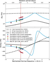 |
Fig. 6 Normalized forcing frequency dependence of the complex quadruploar term of the pressure anomaly field, |
![Mathematical equation: $\[\tilde{q}_{a}\]$](/articles/aa/full_html/2026/07/aa59619-26/aa59619-26-eq14.png)
![Mathematical equation: $\[\tilde{q}_{a}\]$](/articles/aa/full_html/2026/07/aa59619-26/aa59619-26-eq15.png)
![Mathematical equation: $\[\tilde{q}_{a}\]$](/articles/aa/full_html/2026/07/aa59619-26/aa59619-26-eq16.png)
![Mathematical equation: $\[\tilde{q}_{a}\]$](/articles/aa/full_html/2026/07/aa59619-26/aa59619-26-eq17.png)
4 Discussion and conclusion
In this study, we highlight the significant effect of topography on the atmospheric thermal tides and the rotational evolution of planets. Taking the example of Venus, we show that the surface pressure anomalies created by the thermal tides are amplified over lowlands and reduced over highlands because of the overlying atmospheric mass involved in the dynamic. Moreover, the surface topography directly influences the amplitude and the diurnal variability of the atmospheric thermal torque. Where simulations without topography exhibit small variations over a day, the presence of topography creates strong modulations in the torque that are directly related to the large-scale topographies at low and mid latitudes. As for the pressure anomaly, the torque is reduced when the tidal negative anomaly is above highlands and increased over lowlands. Since this effect influences the current thermal tides, it must also be taken into account when modeling the long-term rotational evolution of the planet. Indeed, the presence of topography directly modifies the relationship between the forcing frequency and the atmospheric thermal torque. By updating the empirical law proposed by Leconte et al. (2015), we have shown that the general behavior remains the same, but that taking topography into account modifies the scale of this law.
These results highlight that modeling the rotational state and evolution of Venus, and more broadly those of other planets and exoplanets, without accounting for topographic evolution can lead to significant inaccuracies. Events such as TPW, global resurfacing episodes, or the formation of major topographies, could have significantly modified the atmospheric thermal torque over the history of Venus. While day-to-day variations may be negligible, the cumulative effects over billions of years can strongly influence the overall rotational evolution of the planet. In addition, this study has direct implications for understanding the current rotational state of Venus and its potential equilibrium state. Indeed, if Venus recently experienced variations in the atmospheric thermal torque, they must be compensated for by an evolution of the rotation period to reach equilibrium. However, in the context of a TPW, the timescale required to reach an equilibrium state is expected to exceed the timescale of the TPW itself. Therefore, if a single TPW has occurred in the past, Venus’ rotation would likely have the time to readjust to the modified atmospheric thermal tides. However, if the planet undergoes continuous reorientation, as observed on Earth, the rotational adjustment may never reach the steady equilibrium state.
Therefore, this study brings out the necessity to precisely model the dynamics of the atmospheric thermal tides. For example, the V-PCM used in this study does not account for the planet’s obliquity. Although Venus’ present-day obliquity is small, a TPW event could be accompanied by a change in obliquity that may influence the atmospheric torque. Moreover, if the main features of Venus’ atmospheric dynamics are correctly reproduced by the majority of Venusian global climate models (GCMs), the various GCMs show differences, particularly when assessing the thermal structure of the upper atmosphere as well as the dynamics at low altitudes (Scarica et al. 2019). These discrepancies could strongly affect the modeling of atmospheric thermal tides and emphasize the need to reduce these uncertainties through new observations. For this purpose, the future missions EnVision (ESA), and DaVinci+ (Helbert et al. 2021; Smrekar et al. 2022; Garvin et al. 2022) aim, in part, to study the atmosphere of Venus and better constrain the atmospheric thermal tides. In particular, the Radio Science Experiment proposed by EnVision should be able to study the atmospheric dynamics through the radio occultation experiment, by characterizing the pressure and temperature profiles of the atmosphere above 35 km (Tellmann et al. 2024), and through the gravity experiment, by quantifying the time variations in the gravity field revealing both the effect of gravitational tides and atmospheric thermal tides (Rosenblatt et al. 2021). Such observations would be essential to better characterize the atmospheric thermal tides and the coupling with the solid part of the planet.
Data availability
The data associated with the figures presented in this study are available at https://doi.org/10.5281/zenodo.20644415. Additional data will be made available upon request.
Acknowledgements
This work received support from CNES for the preparation of the ESA EnVision mission (Radio Science Experiment). This research used resources of the GLiCID Computing Facility (Ligerien Group for Intensive Distributed Computing, https://doi.org/10.60487/glicid, Pays de la Loire, France).
References
- Argus, D. F., & Gross, R. S. 2004, Geophys. Res. Lett., 31, L06614 [Google Scholar]
- Auclair-Desrotour, P., Laskar, J., Mathis, S., & Correia, A. C. M. 2017, A&A, 603, A108 [NASA ADS] [CrossRef] [EDP Sciences] [Google Scholar]
- Austin, T. J., O’Rourke, J. G., Izenberg, N., & Silber, E. A. 2025, AGU Adv., 6, e2025AV001906 [Google Scholar]
- Bertaux, J.-L., Khatuntsev, I. V., Hauchecorne, A., et al. 2016, J. Geophys. Res., 121, 1087 [Google Scholar]
- Bills, B. G., Navarro, T., Schubert, G., Ermakov, A., & Górski, K. M. 2020, Icarus, 340, 113568 [NASA ADS] [CrossRef] [Google Scholar]
- Carpenter, R. L. 1964, ApJ, 69, 2 [Google Scholar]
- Correia, A. C., & Laskar, J. 2001, Nature, 411, 767 [NASA ADS] [CrossRef] [Google Scholar]
- Correia, A. C. M., & Laskar, J. 2003, J. Geophys. Res., 108, 5123 [Google Scholar]
- Dumoulin, C., Tobie, G., Verhoeven, O., Rosenblatt, P., & Rambaux, N. 2017, J. Geophys. Res., 122, 1338 [Google Scholar]
- Fu, R. R., & Kent, D. V. 2018, EPSL, 490, 20 [Google Scholar]
- Fukuhara, T., Futaguchi, M., Hashimoto, G. L., et al. 2017, Nat. Geosci., 10, 85 [Google Scholar]
- Garvin, J. B., Getty, S. A., Arney, G. N., et al. 2022, PSJ, 3, 117 [NASA ADS] [Google Scholar]
- Ghelichkhan, S., Hoggard, M. J., Richards, F. D., et al. 2025, GJI, 242, ggaf197 [Google Scholar]
- Gillmann, C., & Tackley, P. 2014, J. Geophys. Res., 119, 1189 [Google Scholar]
- Gold, T., & Soter, S. 1969, Icarus, 11, 356 [NASA ADS] [CrossRef] [Google Scholar]
- Goldreich, P., & Peale, S. J. 1970, AJ, 75, 273 [Google Scholar]
- Goldstein, R. M. 1964, AJ, 69, 12 [Google Scholar]
- Greff-Lefftz, M. 2004, GJI, 159, 1125 [Google Scholar]
- Helbert, J., Maturilli, A., Dyar, M. D., & Alemanno, G. 2021, Sci. Adv., 7, eaba9428 [Google Scholar]
- Herrick, R. R., Sharpton, V. L., Malin, M. C., Lyons, S. N., & Feely, K. 1997, in Venus II: Geology, Geophysics, Atmosphere, and Solar Wind Environment, eds. S. W. Bougher, D. M. Hunten, & R. J. Phillips, 1015 [Google Scholar]
- Herrick, R. R., Bjonnes, E. T., Carter, L. M., et al. 2023, Space Sci. Rev., 219, 29 [Google Scholar]
- Hu, H., van der Wal, W., & Vermeersen, L. L. A. 2017, J. Geophys. Res., 122, 2745 [Google Scholar]
- Lai, D., Lebonnois, S., & Li, T. 2024, J. Geophys. Res., 129, e2023JE008253 [Google Scholar]
- Lebonnois, S., Hourdin, F., Eymet, V., et al. 2010, J. Geophys. Res., 115, E06006 [Google Scholar]
- Lebonnois, S., Sugimoto, N., & Gilli, G. 2016, Icarus, 278, 38 [Google Scholar]
- Leconte, J. 2018, Nat. Geosci., 11, 168 [Google Scholar]
- Leconte, J., Wu, H., Menou, K., & Murray, N. 2015, Science, 347, 632 [NASA ADS] [CrossRef] [Google Scholar]
- Lefèvre, M., Spiga, A., & Lebonnois, S. 2020, Icarus, 335, 113376 [Google Scholar]
- Margot, J.-L., Campbell, D. B., Giorgini, J. D., et al. 2021, Nat. Astron., 5, 676 [NASA ADS] [CrossRef] [Google Scholar]
- Martinez, A., Lebonnois, S., Millour, E., et al. 2023, Icarus, 389, 115272 [Google Scholar]
- Matsuyama, I., Nimmo, F., & Mitrovica, J. X. 2014, Annu. Rev. Earth Planet. Sci., 42, 605 [Google Scholar]
- Mitrovica, J. X., Wahr, J., Matsuyama, I., & Paulson, A. 2005, GJI, 161, 491 [Google Scholar]
- Musseau, Y., Tobie, G., Dumoulin, C., et al. 2024, Icarus, 422, 116245 [Google Scholar]
- Navarro, T., Schubert, G., & Lebonnois, S. 2018, Nat. Geosci., 11, 487 [Google Scholar]
- Patočka, V. 2021, J. Geophys. Res., 126, e2021JE006948 [Google Scholar]
- Patočka, V., Maia, J., & Plesa, A.-C. 2025, AGU Adv., 6 [Google Scholar]
- Phillips, R. J., Raubertas, R. F., Arvidson, R. E., et al. 1992, J. Geophys. Res., 97, 15923 [Google Scholar]
- Revol, A., Bolmont, E., Tobie, G., et al. 2023, A&A, 674, A227 [NASA ADS] [CrossRef] [EDP Sciences] [Google Scholar]
- Rosenblatt, P., Dumoulin, C., Marty, J.-C., & Genova, A. 2021, Remote Sens., 13, 1624 [Google Scholar]
- Salazar, A. M., & Wordsworth, R. 2024, PSJ, 5, 218 [Google Scholar]
- Scarica, P., Garate-Lopez, I., Lebonnois, S., et al. 2019, Atmosphere, 10, 10 [Google Scholar]
- Smith, W. B. 1963, AJ, 68, 15 [CrossRef] [Google Scholar]
- Smrekar, S., Hensley, S., Nybakken, R., et al. 2022, IEEE Aero. Conference, 1 [Google Scholar]
- Steinberger, B. 2008, Nature, 452, 620 [CrossRef] [Google Scholar]
- Strom, R. G., Schaber, G. G., & Dawson, D. D. 1994, J. Geophys. Res., 99, 10899 [Google Scholar]
- Tellmann, S., Oschlisniok, J., Pätzold, M., Dumoulin, C., & Rosenblatt, P. 2024, EPSC2024-796 [Google Scholar]
- Wieczorek, M. A., & Meschede, M. 2018, Geochem. Geophys. Geosyst., 19, 2574 [Google Scholar]
- Wu, P., & Peltier, W. R. 1984, GJI, 76, 753 [Google Scholar]
Appendix A Additional figure
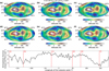 |
Fig. A.1 H-15-150 simulation (αlat = 15° and αlon = 150°). Top: Comparative maps showing the reconstructed topography from the first five spherical harmonic orders of altitude and the quadrupolar pressure anomaly at various times of day. The topography is displayed as the colored background, while the pressure anomaly is indicated by red (positive) and blue (negative) contours. Bottom: Atmospheric thermal torque as function of the subsolar point longitude. The dotted red lines indicate the longitude of the subsolar point for the six maps presented in the top panel. Letter A-E indicate the locations of the principal provinces of Venus, as defined in the caption of Fig. 1. |
All Tables
Numerical values of q0 and ω0 derived from VGCM simulations compared to Leconte et al. (2015) results.
All Figures
|
Fig. 1 Creation of synthetic topography fields using rotations of Venus’ current topography. Left: illustration of the angles, αlat and αlon, that define the reorientation applied on the topography. The angle αlat defines the latitude of the geographic pole with respect to the rotational axis. The angle αlon defines the position of the 0° longitude relative to its present-day position. The present-day topography is therefore given by αlat = 0° and αlon = 0°. Right: topographic maps for several configurations. (a) αlat = 0° and αlon = 0° (current topography). (b) αlat = 0° and αlon = 150°. (c) αlat = 75° and αlon = 0°. (d) αlat = 75° and αlon = 150°. The transition from (a) to (b) correspond to a variation in αlon resulting in a longitudinal rotation of the topography. The transition from (a) to (c) correspond to a variation in the αlat angle resulting in a latitudinal rotation. The transition from (a) to (d) represents a combined variation in both angles. Letter A–E indicate the locations of the principal provinces of Venus, with A=A phrodite Terra, B=Ishtar Terra, C=Alta Regio, D=Guinevere Planitia, and E=Lavinia Planitia. |
| In the text | |
|
Fig. 2 Atmospheric thermal torque over one Venusian day for three simulations. Blue and red lines display the torque for a reference simulation with (H-00-000) and without topography, respectively. The green line corresponds to the torque obtained without topography by Leconte et al. (2015). The daily mean values of these three torques are depicted in dashed lines. |
| In the text | |
|
Fig. 3 Topographic (panels a–c) and pressure anomaly (panels d–f) maps for three different topographic configurations. (a) and (d): αlat = 15° and αlon = 30° (H-15-030). (b) and (e): αlat = 75° and αlon = 210° (H-75-210).(c) and (f): αlat = 90° and αlon = 0° (H-90-000). The black lines display the topographic contours in all panels, while the thick dotted black line indicates the longitude of the subsolar point. Letter A–E indicate the locations of the principal provinces of Venus, as defined in the caption of Fig. 1. |
| In the text | |
|
Fig. 4 H-00-000 simulation (current topography, αlat =0° and αlon =0°). Top: comparative maps showing the reconstructed topography from the first five spherical harmonic orders of altitude and the quadrupolar pressure anomaly at various times of day. The topography is displayed as the colored background, while the pressure anomaly is indicated by red (positive) and blue (negative) contours. Bottom: atmospheric thermal torque as function of the subsolar point longitude. The dotted red lines indicate the longitude of the subsolar point for the six maps presented in the top panel. Letter A–E indicate the locations of the principal provinces of Venus, as defined in the caption of Fig. 1. |
| In the text | |
|
Fig. 5 Equilibrium rotation period as function of the atmospheric thermal torque computed for all the investigated topographic configurations. The current rotation period is indicated by the dotted pink line. The three-layer viscosity profile (composed by a crust, an upper mantle, and a 10 times more viscous lower mantle above a liquid core) used to compute the equilibrium rotation period is also represented in the upper right corner. |
| In the text | |
|
Fig. 6 Normalized forcing frequency dependence of the complex quadruploar term of the pressure anomaly field, |
| In the text | |
|
Fig. A.1 H-15-150 simulation (αlat = 15° and αlon = 150°). Top: Comparative maps showing the reconstructed topography from the first five spherical harmonic orders of altitude and the quadrupolar pressure anomaly at various times of day. The topography is displayed as the colored background, while the pressure anomaly is indicated by red (positive) and blue (negative) contours. Bottom: Atmospheric thermal torque as function of the subsolar point longitude. The dotted red lines indicate the longitude of the subsolar point for the six maps presented in the top panel. Letter A-E indicate the locations of the principal provinces of Venus, as defined in the caption of Fig. 1. |
| In the text | |
Current usage metrics show cumulative count of Article Views (full-text article views including HTML views, PDF and ePub downloads, according to the available data) and Abstracts Views on Vision4Press platform.
Data correspond to usage on the plateform after 2015. The current usage metrics is available 48-96 hours after online publication and is updated daily on week days.
Initial download of the metrics may take a while.