


| Issue |
A&A
Volume 710, June 2026
|
|
|---|---|---|
| Article Number | A220 | |
| Number of page(s) | 12 | |
| Section | Astrophysical processes | |
| DOI | https://doi.org/10.1051/0004-6361/202659594 | |
| Published online | 22 June 2026 | |
Kelvin waves over a differentially rotating spherical shell
IRAP, Université de Toulouse, CNRS, UPS, CNES, 14, avenue Édouard Belin, F-31400 Toulouse, France
★ Corresponding authors: This email address is being protected from spambots. You need JavaScript enabled to view it.
; This email address is being protected from spambots. You need JavaScript enabled to view it.
Received:
24
February
2026
Accepted:
14
April
2026
Abstract
Context. Be stars are currently viewed as B-type stars surrounded by a disc fuelled by the star itself during episodic excretion events. The origin of these events is poorly understood.
Aims. This study aims to determine whether surface equatorial Kelvin waves can be unstable and therefore can play a role in triggering the Be phenomenon.
Methods. We first derived an analytical expression for gravito-inertial modes in the shallow water framework. We then numerically investigated the evolution of equatorial Kelvin modes as the system parameters varied. We extended the study to thick-layer configurations with a constant-density fluid. We then analysed the stability of these modes under differential rotation and viscous effects.
Results. We show that equatorial Kelvin waves still exist in a spherical shell of finite thickness, but their equatorial confinement is weaker. At low azimuthal wave numbers, Kelvin waves lie in the inertial-wave frequency band and therefore exhibit specificities of inertial waves, such as shear layers associated with singularities of the Poincaré equation. These shear layers constitute new dissipative structures for Kelvin waves. When a radial (shellular) differential rotation is imposed, we show that equatorial Kelvin waves can be destabilised, provided that differential rotation and viscosity are in an appropriate range. We trace back the non-monotonic behaviour of the instability growth rate to the rise of a critical layer where the fluid azimuthal velocity equals the phase speed of the surface waves.
Conclusions. This study provides new insights into the behaviour of equatorial Kelvin waves in astrophysics, particularly in rapidly rotating stars. The results reinforce the idea that gravito-inertial waves, and more specifically the equatorial Kelvin waves, can be unstable and thus constitute key components in the mechanisms leading to the Be phenomenon.
Key words: hydrodynamics / instabilities / waves / stars: emission-line, Be / stars: rotation
© The Authors 2026
 Open Access article, published by EDP Sciences, under the terms of the Creative Commons Attribution License (https://creativecommons.org/licenses/by/4.0), which permits unrestricted use, distribution, and reproduction in any medium, provided the original work is properly cited.
This article is published in open access under the Subscribe to Open model. This email address is being protected from spambots. You need JavaScript enabled to view it. to support open access publication.
1. Introduction
Kelvin waves are a class of waves that contain a component of surface gravity waves. However, their definition has varied over time. The first reference to Kelvin’s work on waves is likely found in Cowling (1941), which is dedicated to the non-radial oscillations of a polytropic star. In Kelvin’s original work (Thomson 1863), waves are defined as oscillations of a self-gravitating sphere made of an incompressible fluid (see Lamb 1932, §262), but Cowling did not connect his set of waves to those of Kelvin. In fact, Chandrasekhar & Lebovitz (1963) appear to have been the first to explicitly introduce Kelvin waves into the astrophysical literature. Later, Hurley et al. (1966) performed a full numerical analysis of non-radial oscillations of polytropes and provided the first non-perturbative approach to Kelvin-mode frequencies that fully included compressibility, thus moving a step beyond the works of Chandrasekhar & Lebovitz (1963) and Chandrasekhar (1964). The nomenclature in the astrophysical literature has changed, and these Kelvin modes are now referred to as f-modes (fundamental gravity modes; Cowling (1941)). Robe & Brandt (1966) established the link between Kelvin modes and f-modes. Since then, Cowling’s terminology has prevailed.
Also in 1966, a new Kelvin wave appeared in the literature with the work of Matsuno (1966), who studied the oscillations of the Earth’s atmosphere and oceans. These Kelvin waves refer to two families: coastal Kelvin waves and equatorial Kelvin waves. They are also related to Kelvin’s work (Thomson 1880), which is dedicated to the study of horizontal oscillations of a thin fluid layer in a rotating frame. Their study was a follow-up of Laplace’s seminal work on tides (Laplace 1799), which introduced the shallow water approximation (see Sect. 2). Matsuno (1966) revisited the system originally set out by Laplace and introduced a less restrictive assumption than that used by Kelvin, namely the β-plane approximation, which includes a linear variation of the projected rotation vector as a function of latitude. This approximation remains a standard framework in Earth sciences. This new class of Kelvin waves exists only when a background rotation is present. It can be viewed as a special class of gravito-inertial waves1.
Two years after Matsuno’s study, Wallace & Kousky (1968) reported the first observation of equatorial Kelvin waves in the Earth’s stratosphere. Kelvin waves play a major role in terrestrial fluid dynamics, notably through their impact on phenomena such as El Niño (Cushman-Roisin 1994). However, while Kelvin waves have been extensively studied in oceanography and atmospheric sciences, their role in astrophysical contexts remains relatively unexplored and is usually treated as a secondary question. A first in-depth discussion was provided by Townsend (2003), which relied on the traditional approximation of rotation (TAR). Later, while analysing the light curves of α Ophiuchi (Rasalhague) obtained with the Microvariability and Oscillations of STars (MOST) satellite (Walker et al. 2003), Monnier et al. (2010) suggested the possible detection of equatorial Kelvin waves in that star. More recently, Takata et al. (2020) introduced the ‘internal equatorial Kelvin waves’, referring to the role of buoyancy in their dynamics. However, the specificity of equatorial Kelvin waves was revealed by the seminal work of Delplace et al. (2017) who underline their topological nature. These properties and their consequences in stellar physics are studied in very recent works such as Perez et al. (2022, 2025) and Leclerc et al. (2022, 2024). For completeness, we should mention that Kelvin waves, in their diverse definitions, have also been studied for their potential efficiency in the emission of gravitational radiation by neutron stars (Andersson 2021).
The stability of equatorial Kelvin waves is of great interest given their known properties and their robustness arising from their topological nature, particularly when rotation and gravity combine. Indeed, their prograde nature and equatorial confinement make them interesting candidates for launching matter into orbit around rapidly rotating stars, provided that they can be destabilised by differential rotation. Hence, they may be important contributors to the Be phenomenon, which is now associated with near-critically rotating B stars (Porter & Rivinius 2003). The purpose of this paper is to explore this possibility using the simplified setup of an incompressible fluid in a rotating spherical shell.
The paper is organised as follows. To start from a well-posed problem, we first investigate how equatorial Kelvin waves transform when moving from the shallow water approximation (Sect. 2) to a thick fluid spherical shell mimicking a stellar envelope (Sect. 3). We then impose a shellular differential rotation on this fluid layer, including viscosity, and investigate the stability of the waves (Sect. 4). We conclude the paper with the conclusions and outlook.
2. The shallow water system
To investigate Kelvin modes in a fluid inside a spherical shell rotating at constant angular velocity Ω = Ωez, we begin with the shallow water system, where these modes have been studied.
The shallow water system considers a thin layer of fluid of thickness H0, which is very small compared to the wavelength of the modes. In this case, the equations can be simplified by neglecting the radial component of the velocity. The radial momentum equation ensures predominant hydrostatic balance in the vertical direction.
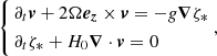
These two simplifications imply the removal of the tangential component of the rotation vector, which means that the shallow water system falls within the framework of the traditional approximation of rotation2. Furthermore, the pressure variable can be expressed as a function of a surface elevation variable ζ*. The linearised shallow water equations thus read as (but see also Cushman-Roisin 1994)
 (1)
(1)
for momentum and mass conservation, respectively. The Coriolis angular frequency is given by 2Ω, and g is the effective gravity, defined as the sum of the gravitational and centrifugal accelerations. The velocity field is v = vθeθ + vϕeϕ.
Matsuno (1966) found solutions of the shallow water system (1) using the β-plane approximation. He identified four types of gravito-inertial modes: Poincaré modes, Rossby modes, Kelvin modes, and Yanai modes, which we now briefly discuss in the context of spherical geometry.
Since perturbations develop over an axisymmetric background, we can write their components as
 (2)
(2)
where θ is the co-latitude and ϕ is the longitude. Next, we introduce the variable μ = cos θ and define the following non-dimensional quantities:
 (3)
(3)
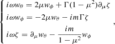
Introducing  , we rewrite (1) as
 (4)
(4)
with
 (5)
(5)
System (4) thus depends on a single non-dimensional parameter, Γ, which can also be expressed as Γ = (c/ceq)2, where  is the phase and group velocities of surface gravity waves in a non-rotating plane layer, and ceq is the background equatorial velocity.
2.1. Rossby modes
Rossby modes, also called planetary waves, are a subclass of inertial modes whose restoring force is the Coriolis force. They are characterised by their low frequency (ω ≪ 1) and their 2D nature, which arises naturally in the shallow water approximation.
Unlike gravity modes, Rossby waves do not require a free surface to exist. They are also supported in a fluid shell with a rigid, non-deformable upper boundary (Longuet-Higgins 1964). Thus, we assume ζ → 0 but keep Γζ finite to preserve the pressure perturbation associated with the velocity field. Hence, the third equation of (4) reduces to
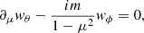
which implies a divergence-free velocity field. This motivated the introduction of a stream function χ, through which we express the velocity field as v = ∇ × (χer). Thus,

We can then rewrite system (4) in terms of the stream function as

where Δh is the horizontal Laplacian, whose eigenfunctions are the spherical harmonics. Setting χ = χmℓYℓm, we deduce the dispersion relation of Rossby modes, namely
 (6)
(6)
This relation is well-known (Longuet-Higgins 1964; Rieutord 2015). These waves are retrograde and their frequency is bounded |ω|≤1. We also note that these waves are independent of Γ.
2.2. Poincaré modes
In the absence of rotation, an incompressible fluid with a free surface supports surface gravity waves. These waves occupy the high-frequency band, and their dispersion relation depends on the fluid depth. However, when rotation is present, the Coriolis force modifies their dynamics. In the shallow water approximation combined with the so-called f-plane approximation, their dispersion relation is ω2 = c2k2 + f2, where k is the wave number and f = 2Ω sin θ is the projected Coriolis frequency at latitude θ. These waves are commonly known as Poincaré waves (Cushman-Roisin 1994; Delplace et al. 2017).
When the domain is the whole surface of the sphere, Poincaré modes are rotation-modified surface gravity modes, where both gravity and the Coriolis force act as restoring forces. Unlike planetary waves, their frequency is unbounded.
In this high-frequency regime, the dominant solutions correspond to pure surface gravity modes with a zeroth-order frequency given by

which is associated with the spherical harmonics Yℓm as the eigenfunction. Introducing a first-order correction due to rotation, the frequency becomes
 (7)
(7)
or, with dimensional quantities
 (8)
(8)
The corresponding eigenfunctions are Hough functions (Wang et al. 2016), which reduce to spherical harmonics in the high frequency limit. We give the derivation of (7) in Appendix A.
2.3. Equatorial modes
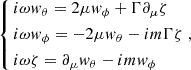
The spectral space associated with equations (4) has topological properties that are related to the breaking of the time-reversal symmetry. This leads to two families of equatorially trapped prograde modes, namely the Kelvin and Yanai modes3 (Delplace et al. 2017). Kelvin modes are equatorially symmetric, whereas Yanai modes are anti-symmetric. Because of their topological origin, these two series of modes are robust to variations in the background physics. Hence, we expect their presence if the background is no longer as simple as in the shallow water model. In the following, we extend the shallow water model to a differentially rotating thick layer. However, as a preliminary step, we first derived the dispersion relation of these modes. To this end, since these modes are equatorially trapped, we assume μ2 ≪ 1, so that (4) can be simplified as follows:
 (9)
(9)
which are the β-plane equations (e.g. Matsuno 1966; Cushman-Roisin 1994).
2.3.1. Kelvin modes
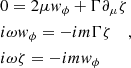
Among equatorial solutions, Matsuno (1966) identified the Kelvin mode as a particular solution of the shallow water system in which the latitudinal velocity vanishes. Thus, setting wθ = 0, we obtain
 (10)
(10)
from which we derive the dispersion relation
 (11)
(11)
We chose the sign to ensure the non-divergence of the corresponding eigenfunction,
 (12)
(12)
The eigenfunction becomes equatorially trapped as Γ decreases, i.e. as the rotation rate increases. Equation (11) shows that Kelvin waves are prograde and regularly spaced in frequency. Equation (12) shows that the latitudinal width of these equatorial waves scales as Γ1/4.
2.3.2. Yanai modes
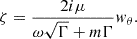
The second equatorially trapped wave in the shallow water system is the Yanai mode. It is anti-symmetric with respect to the equator for wϕ and ζ, and has a non-zero meridional velocity at the equator (Zeitlin 2018). We retrieve it by imposing
 (13)
(13)
This leads to a Gaussian solution for wθ, namely
 (14)
(14)
which is symmetric with respect to the equator, as expected. The dispersion relation of these modes reads
 (15)
(15)
2.4. Numerical solutions
To further illustrate and visualise the eigenspectrum of the shallow water system, we next solved (4) numerically. To this end, we discretised (4) on the Gauss-Lobatto collocation grid associated with Chebyshev polynomials (Fornberg 1998). This spectral discretization ensures rapid convergence of the numerical solutions. We then solved the resulting eigenvalue problem with the classical QZ algorithm (e.g. Valdettaro et al. 2007; Chatelin 2012).
The value of Γ plays a crucial role in the shape of gravito-inertial modes, especially for equatorial modes. On the one hand, Γ determines their equatorial confinement, as shown in (12) and (14). The smaller Γ, the more confined the Kelvin and Yanai modes are at the equator. On the other hand, equatorial modes are characterised by frequencies that asymptotically approach those of other gravito-inertial modes. Specifically, Kelvin modes connect Poincaré modes at high wave numbers, while Yanai modes transit between Rossby modes and Poincaré modes. Figure 1 illustrates this. If Γ is too large, the dispersion relation of gravito-inertial modes shows no distinction for equatorial modes, revealing only Poincaré and Rossby modes4. For equatorial modes to stand out among other modes, Γ must be sufficiently small, typically less than 10−1.
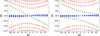 |
Fig. 1. Dispersion relation of gravito-inertial modes in the shallow water system for Γ = 0.01. Left: Eigenfrequency of modes symmetric with respect to the equator as a function of the azimuthal wave number m. Right : Same as the left panel but for antisymmetric modes. Red dots show Poincaré modes, blue dots show Rossby modes, and green dots show Kelvin (left) and Yanai (right) modes. |
2.5. Planetary and stellar context
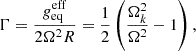
The shallow water model demonstrates the existence of Kelvin and Yanai modes when the parameter Γ is small compared to unity. On Earth, the kilometric thickness of the atmosphere or the oceans makes Γ on the order of 10−1, a value at which equatorial modes are expected to be prominent. This has been confirmed through years of oceanic observations. For a rotating main-sequence star, no such thin layers exist and surface waves can spread in depth. However, because our study considers Be stars, whose rotation is near critical, the effective equatorial surface gravity is weak. We therefore expect small values of Γ even in a deep layer. Assuming H0 = R/2, we obtain
 (16)
(16)
where  is the effective gravity at the equator and
 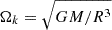 is the Keplerian angular velocity at the same location. For a star rotating at 90% of the critical angular velocity, Γ ∼ 0.1, which is similar to the Earth value. Rapidly rotating intermediate-mass stars evolve at nearly constant angular momentum (Gagnier et al. 2019) and slowly enough to remain in a quasi-steady state. As shown by Mombarg et al. (2024), the ratio Ω2/Ωk2 increases to unity during the main sequence. Hence, equatorially confined Kelvin or Yanai modes should be expected when the star reaches near-critical rotation.
The foregoing considerations prompted us to examine the role of shell thickness on the properties of Kelvin waves. We wanted to determine whether the low value of the Γ parameter was still a sufficient condition for the existence of equatorially confined Kelvin modes.
3. Extension to the thick shell
To appreciate the effects of thickening the fluid layer, we considered a spherical shell of fluid extending from r = η to r = 1, where the outer surface of the shell is free to support gravity waves. Simultaneously, we introduced viscosity to numerically regularise the problem and avoid singularities of inertial modes in the spherical shell. Indeed, as shown in Rieutord & Valdettaro (1997) and Rieutord et al. (2001), the Poincaré equation, which governs the inertial modes of an inviscid rotating fluid, is spatially hyperbolic and has mainly singular solutions, wrapped around attractors of characteristics generated by boundary conditions. Viscosity smooths these singularities into oscillating shear layers (Rieutord et al. 2002).
Moreover, we ignored self-gravity, hence working under Cowling’s approximation. Surface gravity waves combined with self-gravity are unstable at sufficiently high rotation rates and allow the bifurcation of the axisymmetric MacLaurin spheroid to triaxial spheroids when rotation is high enough (Chandrasekhar 1969). We neglected these complex matters because our incompressible fluid layer serves as a simple model for describing Kelvin waves in stellar envelopes, which exhibit density variations, entropy stratification, and at least differential rotation. As shown in Appendix B, our uniformly rotating fluid shell is always stable. Hence, we considered the ratio
 (17)
(17)
namely the surface gravity divided by the centrifugal acceleration, and allowed it to be greater or less than unity to explore the physical or mathematical properties of the global modes. As previously observed, γ < 1 is not physically absurd if g refers to the effective gravity in the equatorial region of a rapidly rotating star.
3.1. Mathematical formulation
Consider a fluid particle in a rapidly rotating fluid. Its velocity can be expressed as Ω × r + v, with v small compared to Ω × r. The particle dynamics is characterised by a small Rossby number and is governed by a linear system. Using Ω−1 as the timescale and the outer radius of the shell R as the length scale, the linearised momentum and mass conservation equations in an inertial frame read as
 (18)
(18)
We assumed velocity and pressure perturbations of the form
 (19)
(19)
where λ = τ + iω is the complex eigenvalue. We also introduced the Ekman number,
 (20)
(20)
as a measure of the kinematic viscosity ν.
At the inner boundary r = η, stress-free conditions are imposed, namely,
 (21)
(21)
On the outer free surface, the kinematic boundary condition implies
 (22)
(22)
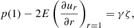
where ζ is the dimensionless elevation of the surface. Since the surface experiences no stress, the dynamical boundary condition imposes
 (23)
(23)
 (24)
(24)
 (25)
(25)
Here, [c] is the shear tensor with cij = ∂iuj + ∂jui and we define γ by (17). We can eliminate the surface elevation, ζ, between the kinematic condition (22) and the pressure condition (23). In doing so, we note that as γ → ∞, the combined boundary condition becomes equivalent to ur = 0, i.e., a rigid boundary, as expected. We also note that the parameters Γ and γ are related by
 (26)
(26)
since H0 = (1 − η)R.
3.2. Numerical method
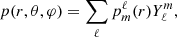
We solved system (18), together with boundary conditions (21-25) numerically using spectral methods. We expanded the pressure field in the usual spherical harmonics as
 (27)
(27)
while we expanded the velocity field on vectorial spherical harmonics as

with

where gradients are taken on the unit sphere. Here, Lmax denotes the truncation order of the spherical harmonics expansion.
We then sampled the radial functions pmℓ, umℓ, vmℓ, and wmℓ on Nr grid points of the Gauss-Lobatto collocation grid associated with Chebyshev polynomials. We determined eigenvalues λ either with the QZ-method for a global calculation or with the incomplete Arnoldi-Chebyshev method for computing specific eigenvalues (e.g. Valdettaro et al. 2007).
3.3. Properties of Kelvin waves in a thick layer
Kelvin waves do not exist without rotation, but they share several properties with surface gravity waves, which they actually are. They are non-dispersive waves in the shallow water limit (see Eq. (11)) and propagate at velocity  , just like surface gravity waves in this limit.
To identify Kelvin waves in the thick spherical shell, we tracked their eigenvalues in the complex plane as the core radius of the shell, η, decreases. Starting at η ≲ 1, we easily identify the equatorial Kelvin wave because of its shallow water frequency. Figure 2 shows that the Kelvin wave can be continuously traced as the core size decreases until the core disappears. In this limit, it joins the spectrum of eigenmodes of the full sphere, which we can derive analytically (e.g. Appendix C and Bryan 1889). In this case, the dispersion relation of the Kelvin waves reads  (note that in the full sphere case Γ = γ).
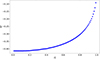 |
Fig. 2. Evolution of the eigenfrequency of the m = 1 Kelvin mode with the size of the core at γ = 1. In the shallow water and full sphere limits, the value given by their corresponding analytic expression, (11) and (C.10) are recovered, respectively. |
In a thick layer, Kelvin waves also behave similarly to surface gravity waves since, for instance, their amplitude decreases faster with depth the shorter their wavelength, as illustrated in Fig. 3. The m = 10 Kelvin mode (Fig. 3 top) shows a smooth, nodeless structure, as in normal surface gravity waves. However, this Kelvin mode lies outside the inertial frequency band in the corotating frame (i.e. |ω|> 2). This is not the case for the m = 3 Kelvin mode (Fig. 3 bottom), which shows features of inertial modes, such as the emission of a shear layer by the critical latitude singularity on the inner boundary (see for instance He et al. 2022). The excitation of this shear layer increases the damping rate of the mode. In the present example, we note that the damping rate of the m = 3 Kelvin mode is larger than that of the m = 10 equivalent (see caption of Fig. 3).
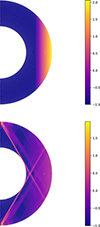 |
Fig. 3. Top: Distribution of kinetic energy on a log10 scale in a meridional section of the spherical shell for the m = 10 Kelvin mode at λ = −1.31 × 10⁻⁵ − 12.31i. Bottom: Same as the top panel but for the m = 3 Kelvin mode at λ = −5.13 × 10⁻⁴ − 3.99i. In both cases η = 0.5, γ = 1, E = 10−7, Nr = 200, and Lmax = 200. |
As with surface gravity waves, Kelvin waves become dispersive as the shell thickens. Figure 4 illustrates this, where we clearly see the increase of phase velocity with increasing thickness of the layer. When the core radius vanishes, that is, when the sphere is full, an analytic expression of the Kelvin modes frequency can be derived (see Appendix C). Figure 4 also shows the continuous relation between the shallow water (η ≃ 1) frequency and the full sphere (η = 0) frequency. We note that the m = 10 Kelvin mode reaches its full-sphere frequency even with a core radius η = 0.7. This is explained by the fact that for such a high m, the eigenfunction has its amplitude mainly close to the upper boundary and almost does not ‘feel’ the presence of the core.
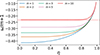 |
Fig. 4. Evolution of the phase velocity of Kelvin modes with various m in the co-rotating frame as a function of core size η for γ = 1, E = 10−3, and Nr = Lmax = 20. The dashed red line shows the phase velocity of the m = 10 Kelvin mode in the full-sphere case. |
Another view of the dispersive effect of the finite thickness of the fluid layer is the frequency difference between consecutive Kelvin modes. In the shallow water case this is a constant quantity that can be used to identify a series of Kelvin modes in photometric data (e.g. Monnier et al. 2010). In Fig. 5 we show how this frequency difference evolves with the size of the core and that it is not the same for low azimuthal wave numbers (i.e. when m ≲ 10).
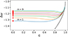 |
Fig. 5. Frequency difference Δω = ωm + 1 − ωm between two consecutive Kelvin modes as a function of core radius. Red dots show the values for the full sphere case as derived from (C.10), while the dashed black line shows the asymptotic shallow-water case. Parameters are γ = 1, E = 10−3 with Nr = Lmax = 20. |
As expressed in (12), within the limits of the shallow water approximation, the eigenfunction of Kelvin modes is a Gaussian centred on the equator. When the layer thickens, the surface shape of Kelvin modes gradually transits towards the sinmθ-shape, which characterises the surface eigenfunction of the Kelvin mode in the full sphere. We illustrate this in Fig. 6. In the shallow water regime, the meridian profile of the eigenfunction does not depend on the azimuthal wave number m and is only a function of the parameter Γ. When the spherical shell thickens, the latitudinal extension of the Kelvin wave depends on m and somehow weakens its dependence on Γ. When the core disappears, the latitude dependence is purely that of the associate Legendre polynomial Pmm(cos θ), that is, in sinmθ.
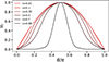 |
Fig. 6. Radial velocity profile at the spherical-shell surface shown as a function of colatitude θ for the m = 1-Kelvin wave at various core sizes. The parameters are γ = 1, E = 10−3, Nr = 30, and Lmax = 60. |
4. Influence of differential rotation
In the previous section we showed that Kelvin waves remain identifiable in a thick layer with a latitudinal spread that increases with the layer thickness similarly to the dispersion in phase velocity. We next investigated whether these surface waves could be destabilised if the background flow differs from a solid-body rotation. We aimed to determine whether the ubiquitous differential rotation of stellar envelopes could destabilise Kelvin waves. We neglected Yanai waves because we expected them to be more stable than Kelvin waves. Indeed, sampling their eigenvalue shows that the damping rate of Yanai modes is generally larger than that of Kelvin modes. Yanai modes are anti-symmetric with respect to the equator; for similar m, their global wave number is higher than that of Kelvin modes, making them presumably more damped. This is consistent with other examples in fluid mechanics where anti-symmetric modes are more stable than symmetric ones (e.g. in thermal convection, Zhang & Busse 1987; Chandrasekhar 1961).
Regarding differential rotation in early-type stars, Espinosa Lara & Rieutord (2013) showed that it results from radiative envelope baroclinicity. The resulting shear is latitudinal and radial, but the latter is usually stronger. For simplicity, we restricted our modelling of differential rotation to a shellular profile, thus depending only on the radial coordinate. We next investigated the stability conditions of Kelvin modes over this type of flows.
4.1. Equations of motion
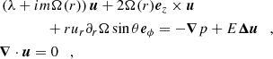
Perturbations evolving over a shellular differential rotation satisfy the following momentum and mass conservation non-dimensional equations, written in an inertial frame:
 (28)
(28)
where we scaled the angular velocity by its surface value. We used the outer radius of the shell as the length scale. We assumed velocity and pressure perturbations to be proportional to exp(λt + imφ).
We chose the background shellular rotation to be
 (29)
(29)
which satisfies Ω(1) = 1, and we introduce the new parameter Ωη = Ω(η), namely the rotation rate at the core boundary. This parameter controls the strength of the differential rotation.
Profile (29) also verifies ∂rΩ(r = 1) = 0, so that it exerts no viscous stress at the surface, as required. This profile thus combines the simplicity of a polynomial radial dependence and the right behaviour near the surface. To mimic envelope differential rotation in more realistic models (e.g. Espinosa Lara & Rieutord 2013), we considered Ωη > 1, hence decreasing rotation rates with radius.
The strength of the differential rotation Ωη should not be too high, as we did not want our set-up to be unstable with respect to centrifugal (Taylor-Couette) instability (e.g. Drazin & Reid 1981). This instability involves axisymmetric perturbations and redistributes the fluid’s angular momentum. Since it develops on a dynamical time scale, it is unlikely to be active in a star. In fact, we assume that profile (29) represents a large-scale differential rotation as driven by baroclinicity and possibly including small-scale turbulence generated by shear instabilities. In Appendix D we show that if
 (30)
(30)
the differential rotation is stable with respect to the centrifugal instability. We therefore limited the strength of the differential rotation with (30).
Concerning the boundary conditions for the perturbations, we kept the same ones as in the uniform rotation case, but modified condition (25) to account for the variations of Ω, such that
 (31)
(31)
where ζ is the radial elevation of the surface as introduced in (3).
4.2. Destabilisation of Kelvin modes
As demonstrated in Appendix B, the gravito-inertial modes of our system are stable in the case of solid-body rotation. As illustrated in Fig. 7, this is no longer the case when a shellular differential rotation is present. We plot the growth rate τ = ℜe(λ) of three Kelvin modes as a function of the Ekman number E (the non-dimensional kinematic viscosity) or the strength of the differential rotation Ωη. Figure 7 (top) clearly shows that for a given differential rotation, there is a critical Ekman number below which a Kelvin mode becomes unstable, and the higher the azimuthal wave number m, the lower the critical Ekman number (as expected). Conversely, for a given Ekman number, there is a critical Ωη beyond which a Kelvin mode becomes unstable.
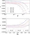 |
Fig. 7. Top: Growth rate τ = ℜe(λ) of selected Kelvin modes as a function of the Ekman number E, for Ωη = 2, Γ = 0.01, and η = 0.18. Bottom: Same as the top panel but as a function of differential rotation parametrized by Ωη, with E = 10−5. The numerical resolution is Nr = Lmax = 100. |
4.3. Origin of the instability
The growth rate of the modes of our system can be expressed using the momentum equation in (28). To do so, we took the dot product of this equation with the complex conjugate of the velocity field, u*, and integrated the equation over the fluid volume. After some rearrangement of the terms, we obtain:
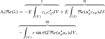 (32)
(32)
where
 (33)
(33)
is a positive-definite term. The first integral is the bulk viscous dissipation, which is always negative, as expected (we used Einstein implicit summation on repeated indices). The second term is a surface integral with no obvious sign. Using the surface boundary condition (31), we note that it relates to the differential rotation via Ω″(1) and to the phase difference between ur and uφ through the kinematic boundary condition (22). We numerically investigated its role in the instability and found that it is always negative, thus playing a stabilising role, although we could not prove that this is always the case. The third term is responsible for the instability of Kelvin modes. Because Ω′(r) < 0 over the volume, modes can become unstable when ℜe(uruφ*) is positive or, equivalently, when the phase difference between ur and uφ is less than π/2 over most of the volume.
To better characterise this instability, we investigated the dependence of τ = ℜe(λ) as a function of the differential rotation parameter Ωη for various Ekman numbers. We recall that as Ωη increases, the core rotation rate increases as the differential rotation. Figure 8 shows the variation of τ with Ωη for three Ekman numbers. The shape of the curve remains similar for the Ekman numbers considered. We clearly see that for sufficiently low E, τ is positive when Ωη is large enough; however, remarkably, τ becomes negative again when Ωη is too large. Since τ is the sum of three integrals, its behaviour can be explained by the dependence of these integrals on Ωη. Figure 9 shows the variations of the bulk and surface viscous integrals with Ωη. The viscous contribution varies monotonically with Ωη, the damping effect being more important when E and Ωη increase. Figure 10 shows that the variations of τ come from the coupling integral, which first increases with Ωη and then decreases if Ωη ≳ 5. Figures 11 and 12 summarise this behaviour of the growth and damping rate. There, a Kelvin wave becomes unstable below a critical Ekman number, but this is conditioned by the strength of the differential rotation, which must satisfy Ωm < Ωη < ΩM, where the bounds Ωm and ΩM depend on the Ekman number.
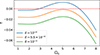 |
Fig. 8. Evolution of τ, the real part of the eigenvalue, for the m = 5 Kelvin mode as a function of Ωη, for three Ekman numbers. The parameters are γ = 2, Nr = 100, and Lmax = 60. |
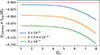 |
Fig. 9. Evolution of the sum of the viscous integrals (I) and (II) in (32) as a function of Ωη for the m = 5 Kelvin mode for three Ekman numbers. The parameters are γ = 2, Nr = 100, and Lmax = 60. |
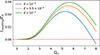 |
Fig. 10. Evolution of the coupling integral (III) in equation (32) as a function of Ωη for the m = 5 Kelvin mode for three Ekman numbers. The parameters are γ = 2, Nr = 100, and Lmax = 60. |
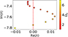 |
Fig. 11. Evolution of the eigenvalue of the m = 5 Kelvin mode in the complex plane. The parameters are γ = 2, η = 0.18, E = 1 × 10⁻⁴, Nr = 100, and Lmax = 100. |
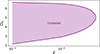 |
Fig. 12. Stability diagram of the m = 5 Kelvin mode at η = 0.18 and γ = 2. The purple region denotes the unstable domain in the explored parameter space and forms a single connected region. The instability does not exist beyond a critical Ekman number E ≈ 5 × 10⁻⁴. |
The foregoing situation resembles shear flow instabilities where a critical layer plays a crucial role. The critical layer is the location where the phase speed of the wave matches that of the background flow. In our case, the critical layer lies on a sphere of radius rc such that
 (34)
(34)
Figure 13 illustrates the wave and critical layer interactions. We first note that as differential rotation strengthens, the critical layer moves towards the surface. Indeed, as shown in Fig. 11, the wave frequency does not vary much when Ωη increases by a factor of ∼4, hence condition (34) is satisfied with an approximately constant Ω(rc), requiring a larger rc as Ωη increases (since Ω is a decreasing function of r).
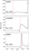 |
Fig. 13. Radial profiles of the coupling term in the equatorial plane θ = π/2, at longitude ϕ = 0, for an m = 5-Kelvin mode and for three differential rotations. The parameters are γ = 2, E = 1 × 10⁻⁵, η = 0.18, Nr = 100, and Lmax = 100. Inertial frame eigenvalues are λ = −2.968 × 10⁻³ − 7.372i for Ωη = 2 implying rcri = 0.435; λ = 1.231 × 10⁻² − 7.591i for Ωη = 5 implying and rcri = 0.704. λ = −4.083 × 10⁻² − 7.929i, for Ωη = 8 implying rcri = 0.762. |
Figure 13 also shows that at high differential rotation (here at Ωη = 8), the internal part of the Kelvin wave is trapped around the critical layer. This part of the perturbation displays a shear layer, whose width scales as E0.4 in this example. This shear layer is reminiscent of what occurs in plane-parallel shear flows: in an inviscid plane-parallel shear flow, the critical layer is the location of a singularity in the perturbations, which is regularised by viscosity into a thin shear layer (Drazin & Reid 1981; Charru 2011). Numerical exploration of Kelvin waves shows that, at least for some parameters, their instability can also disappear when the Ekman number is sufficiently low, as illustrated in Fig. 14. This property can be understood qualitatively from the scaling of the shear-layer width, which makes the coupling integral (III in Eq. (32)) decay more rapidly with E than the viscous integrals. Here we encounter the double role of a critical layer, which can be either destabilising or stabilising, as shown in other contexts (e.g. Riedinger & Gilbert 2014, in ocean dynamics). We did not analyse this instability as it is beyond the scope of this paper, and this constant-density model remains far from the physical conditions met in stars.
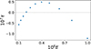 |
Fig. 14. Evolution of the growth rate τ of the m = 1 Kelvin mode as a function of Ekman number E. The frequency is ω ≃ −1.030303. The parameters are η = 0.35, γ−1 = 16.25, Ωη = 1.065 Nr = 200, and Lmax = 200. |
5. Conclusions
We explored the stability of equatorial Kelvin waves propagating over an incompressible, differentially rotating fluid layer contained in a spherical shell. These waves have presumably been detected in the fast rotating star Rasalhague (Monnier et al. 2010) and could also represent a mechanism by which Be stars eject matter in their equatorial plane. Since equatorial Kelvin waves are also special waves of the stellar wave zoo, owing to their topological origin (Delplace et al. 2017), their linear stability is of interest. We did not consider Yanai waves, the anti-symmetric counterpart of Kevin waves, since they are expected to be more stable, as suggested by the cases we computed. Our simplified model shows that even if Kelvin waves have been studied in the shallow water framework (for terrestrial applications), they still exist when the fluid layer is no longer a thin spherical shell. The key difference is that their equatorial confinement is no longer well pronounced unless the azimuthal wave number is large. We also note that at low azimuthal wave number, their frequency lies in the inertial frequency band. In this case, these waves exhibit features of inertial waves, such as shear layers emitted by the critical-latitude singularity at the inner core boundary. Such shear layers provide an additional source of viscous dissipation.
With this model, we also show that Kelvin waves persist in the presence of a shellular (radial) differential rotation. This differential rotation mimics the shear imposed by the baroclinicity in a stellar radiative envelope. Moreover, we show that Kelvin waves become unstable if the viscosity is not too high and differential rotation is strong enough. However, this instability disappears when either the differential rotation is too strong or the Ekman number is very low. We find that the critical layer associated with each Kelvin wave presumably plays a destabilising or stabilising role. As in plane-parallel shear flows, viscosity is a key parameter. The shear layers that appear when Kelvin waves lie in the inertial frequency band are not sufficiently dissipative to prevent the rise of the instability.
The foregoing results suggest that the instability of Kelvin waves will persist when we relax the simplification of a constant density fluid. In this case, surface gravity waves are replaced by the so-called f-modes, which are also topological waves at low wave numbers (Le Saux et al. 2025). The investigation of these waves with a compressible fluid, which more realistically represents a stellar envelope, is a natural follow-up of this work.
Acknowledgments
We would like to thank the referee very much for constructive remarks, which helped us improve the original manuscript. We are also very grateful to Lorenzo Valdettaro for his help in an early phase of the project and to Armand Leclerc for enlightening discussions on topological waves. The research leading to these results has received funding from the European Research Council (ERC) under the Horizon Europe programme (Synergy Grant agreement N°101071505: 4D-STAR). While partially funded by the European Union, views and opinions expressed are however those of the authors only and do not necessarily reflect those of the European Union or the European Research Council. Neither the European Union nor the granting authority can be held responsible for them. Computations have been possible thanks to HPC resources from CALMIP supercomputing centre (Grant 2025-P0107).
References
- Andersson, N. 2021, Universe, 7, 97 [NASA ADS] [CrossRef] [Google Scholar]
- Bryan, G. 1889, Phil. Trans. R. Soc. Lond., 180, 187 [Google Scholar]
- Chandrasekhar, S. 1961, Hydrodynamic and Hydromagnetic Stability (Oxford: Clarendon Press) [Google Scholar]
- Chandrasekhar, S. 1964, ApJ, 139, 664 [Google Scholar]
- Chandrasekhar, S. 1969, Ellipsoidal Figures of Equilibrium (Yale University Press) [Google Scholar]
- Chandrasekhar, S., & Lebovitz, N. R. 1963, ApJ, 138, 185 [Google Scholar]
- Charru, F. 2011, Hydrodynamic Instabilities (Cambridge University Press) [Google Scholar]
- Chatelin, F. 2012, Eigenvalues of Matrices, Revised Edition (SIAM Classics in Applied Mathematics), 410 [Google Scholar]
- Cowling, T. G. 1941, MNRAS, 101, 367 [NASA ADS] [Google Scholar]
- Cushman-Roisin, B. 1994, An Introduction to Geophysical Fluid Dynamics (Paris: Prentice-Hall) [Google Scholar]
- Delplace, P., Marston, J. B., & Venaille, A. 2017, Science, 358, 1075 [Google Scholar]
- Dintrans, B., Rieutord, M., & Valdettaro, L. 1999, J. Fluid Mech., 398, 271 [Google Scholar]
- Drazin, P., & Reid, W. 1981, Hydrodynamic Stability (Cambridge University Press) [Google Scholar]
- Espinosa Lara, F., & Rieutord, M. 2013, A&A, 552, A35 [NASA ADS] [CrossRef] [EDP Sciences] [Google Scholar]
- Fornberg, B. 1998, A Practical Guide to Pseudospectral Methods (Cambridge University Press) [Google Scholar]
- Gagnier, D., Rieutord, M., Charbonnel, C., Putigny, B., & Espinosa Lara, F. 2019, A&A, 625, A89 [NASA ADS] [CrossRef] [EDP Sciences] [Google Scholar]
- Gerkema, T., Zimmerman, J. T. F., Maas, L. R. M., & van Haren, H. 2008, Rev. Geophys., 46, RG2004 [Google Scholar]
- He, J., Favier, B., Rieutord, M., & Le Dizès, S. 2022, J. Fluid Mech., 939, A3 [Google Scholar]
- Hurley, M., Roberts, P. H., & Wright, K. 1966, ApJ, 143, 535 [Google Scholar]
- Lamb, H. 1932, Hydodynamics (Cambridge Univ. Press) [Google Scholar]
- Laplace, P. S. 1799, Traité de Mécanique céleste (Paris: Duprat) [Google Scholar]
- Le Saux, A., Leclerc, A., Laibe, G., Delplace, P., & Venaille, A. 2025, ApJ, 987, L12 [Google Scholar]
- Leclerc, A., Laibe, G., Delplace, P., Venaille, A., & Perez, N. 2022, ApJ, 940, 84 [Google Scholar]
- Leclerc, A., Laibe, G., & Perez, N. 2024, Phys. Rev. Research, 6, 043299 [Google Scholar]
- Longuet-Higgins, M. S. 1964, Proc. R. Soc. Lond. A, 279, 446 [Google Scholar]
- Longuet-Higgins, M. S. 1968, Phil. Trans. R. Soc. of London Series A, 262, 511 [Google Scholar]
- Margules, M. 1892, in Air motions in a rotating spheroidal shell Transl. into English from Trans. of the Acad. Sci. Vienna, 101, 597 [Google Scholar]
- Matsuno, T. 1966, J. Met. Soc. Japan, 44, 25 [Google Scholar]
- Mombarg, J. S. G., Rieutord, M., & Espinosa Lara, F. 2024, A&A, 683, A94 [NASA ADS] [CrossRef] [EDP Sciences] [Google Scholar]
- Monnier, J. D., Townsend, R. H. D., Che, X., et al. 2010, ApJ, 725, 1192 [NASA ADS] [CrossRef] [Google Scholar]
- Müller, D., & O’Brien, J. J. 1995, Phys. Rev. E, 51, 4418 [Google Scholar]
- Perez, N., Delplace, P., & Venaille, A. 2022, Phys. Rev. Lett., 128, 184501 [NASA ADS] [CrossRef] [Google Scholar]
- Perez, N., Leclerc, A., Laibe, G., & Delplace, P. 2025, J. Fluid Mech., 1003, A35 [Google Scholar]
- Porter, J. M., & Rivinius, T. 2003, PASP, 115, 1153 [Google Scholar]
- Prat, V., Mathis, S., Lignières, F., Ballot, J., & Culpin, P. M. 2017, A&A, 598, A105 [NASA ADS] [CrossRef] [EDP Sciences] [Google Scholar]
- Riedinger, X., & Gilbert, A. D. 2014, J. Fluid Mech., 751, 539 [Google Scholar]
- Rieutord, M. 2015, Fluid Dynamics: An Introduction (Springer), 508 [Google Scholar]
- Rieutord, M., & Valdettaro, L. 1997, J. Fluid Mech., 341, 77 [Google Scholar]
- Rieutord, M., Georgeot, B., & Valdettaro, L. 2001, J. Fluid Mech., 435, 103 [Google Scholar]
- Rieutord, M., Valdettaro, L., & Georgeot, B. 2002, J. Fluid Mech., 463, 345 [NASA ADS] [CrossRef] [Google Scholar]
- Robe, H., & Brandt, L. 1966, Ann. Astrophys., 29, 517 [Google Scholar]
- Takata, M., Ouazzani, R. M., Saio, H., et al. 2020, A&A, 635, A106 [NASA ADS] [CrossRef] [EDP Sciences] [Google Scholar]
- Thomson, W. 1863, Phil. Trans. R. Soc. Lond., 153, 583 [Google Scholar]
- Thomson, W. 1880, Proc. Roy. Soc. Edinburgh, 10, 92 [Google Scholar]
- Townsend, R. H. D. 2003, MNRAS, 340, 1020 [Google Scholar]
- Valdettaro, L., Rieutord, M., Braconnier, T., & Fraysse, V. 2007, J. Comput. Appl. Math., 205, 382 [Google Scholar]
- Walker, G., Matthews, J., Kuschnig, R., et al. 2003, PASP, 115, 1023 [Google Scholar]
- Wallace, J. M., & Kousky, V. E. 1968, J. Atmosph. Sci., 25, 900 [Google Scholar]
- Wang, H., Boyd, J. P., & Akmaev, R. A. 2016, Geosci. Model Dev., 9, 1477 [Google Scholar]
- Zeitlin, V. 2018, Geophysical Fluid Dynamics: Understanding (almost) Everything with Rotating Shallow Water Models, 1st edn. (Oxford: Oxford University Press) [Google Scholar]
- Zhang, K.-K., & Busse, F. 1987, Geophys. Astrophys. Fluid Dyn., 39, 119 [Google Scholar]
Gravito-inertial waves usually refer to waves restored by both buoyancy and the Coriolis force (Dintrans et al. 1999). Kelvin waves are surface gravity waves modified by rotation; thus, they can also be viewed as gravito-inertial waves.
This approximation, also called the TAR, is often used in geophysics and astrophysics to simplify the dynamics of rotating fluids (e.g. Gerkema et al. 2008; Prat et al. 2017).
These modes are prograde in group velocity, but Yanai modes can be retrograde in phase velocity (see Fig. 1).
Several authors have performed detailed studies of the Γ → ∞ limit, known as the Margules limit, including Margules (1892), Longuet-Higgins (1968), Müller & O’Brien (1995), Perez et al. (2025).
Appendix A: Tidal Laplace Equation and Poincaré Modes
As in the classical β-plane approximation, it is possible to combine the full set of shallow water equations (4) into a single equation, known as the Tidal Laplace Equation (e.g. Longuet-Higgins 1968):
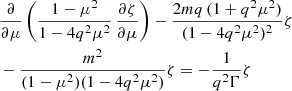 (A.1)
(A.1)
where we have introduced the spin parameter q = 1/ω. In the limit of large frequency (q → 0), this equation simplifies and transforms to the classical spherical Laplacian eigenvalue problem:
 (A.2)
(A.2)
which leads to eigenvalues solutions of:
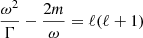 (A.3)
(A.3)
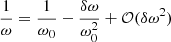
This cubic equation in ω can be solved perturbatively in the limit of large frequencies by introducing a small correction to the zeroth-order solution, which reads
 (A.4)
(A.4)
Introducing the perturbation δω ≪ ω0 and expanding each term to first order:
 (A.5)
(A.5)
 (A.6)
(A.6)
we finally get:
 (A.7)
(A.7)
This expression is the first-order-corrected Poincaré mode frequency in the limit of large ℓ.
Appendix B: The stability of the uniformly rotating viscous spherical shell
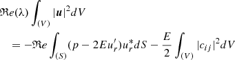
Ignoring self-gravity, perturbations of a uniformly rotating fluid in a spherical shell verify (18) together with boundary conditions (22) and (23). Taking the dot product of the momentum equation with u* (the complex conjugate of u), integrating over the volume of the spherical shell and taking the real part of the equation gives:
 (B.1)
(B.1)
where cij are the components of the shear tensor. Combining boundary conditions (22) and (23) gives:
 (B.2)
(B.2)
where ′ indicates the radial derivative. This allows us to rewrite (B.1) as
![Mathematical equation: $$ \begin{aligned} \mathfrak{R} e(\lambda )\left[\int _{(V)} |\boldsymbol{u}|^2 dV+\frac{1}{\gamma }\int _{(S)} |p-2Eu_r^{\prime }|^2dS\right]&\nonumber \\ = -\frac{E}{2}\int _{(V)}|c_{ij}|^2dV&\end{aligned} $$](/articles/aa/full_html/2026/06/aa59594-26/aa59594-26-eq56.gif) (B.3)
(B.3)
which shows that ℜe(λ) < 0 when the Ekman number E is non-zero, hence when the fluid is viscous.
Appendix C: The full sphere case
Starting from boundary conditions (22) and (23) in the inviscid limit and in the corotating frame, one obtains
 (C.1)
(C.1)
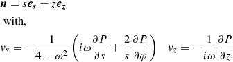
in cylindrical coordinates (s, z, φ) on the unit sphere (r = 1),
 (C.2)
(C.2)
Equation (C.1) can thus be rewritten as
 (C.3)
(C.3)
By introducing the same change of variables as in Rieutord (2015), one finally obtains the following dispersion relation:
![Mathematical equation: $$ \begin{aligned} \left[ 2m +\frac{ \left( 4-\omega ^2 \right)\omega }{\gamma }\right] P^m_l \left(\frac{\omega }{2} \right) =\frac{4-\omega ^2}{2}{P_l^m}^{\prime } \left(\frac{\omega }{2} \right)\; . \end{aligned} $$](/articles/aa/full_html/2026/06/aa59594-26/aa59594-26-eq60.gif) (C.4)
(C.4)
C.1. Kelvin mode
We consider the sectoral mode m = ℓ > 0. From the definition of the associated Legendre polynomials,
 (C.5)
(C.5)
we deduce,
 (C.6)
(C.6)
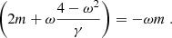
So, (C.4) yields for m = ℓ,
 (C.7)
(C.7)
Noting that ω = −2 is a solution, we rewrite (C.7) as
 (C.8)
(C.8)
The two other roots are
 (C.9)
(C.9)
and we identify the Kelvin mode as the prograde mode, ω < 0, namely
 (C.10)
The other root is that of the first retrograde Poincaré mode.
Appendix D: Centrifugal stability
The flow is stable with respect to centrifugal instability if and only if the specific angular momentum L = s2Ω increases with the distance s to the rotation axis, namely if
 (D.1)
(D.1)
with s = r sin θ. Since
 (D.2)
(D.2)
Condition (D.1) implies
 (D.3)
(D.3)
which is true if this second order equation has no root for r or that
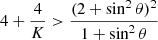 (D.4)
(D.4)
for all θ. Since the RHS is a monotonic increasing function of sin2θ, it reaches a maximum at θ = π/2. Hence, inequality (D.1) is always satisfied if  , which implies (30).
All Figures
|
Fig. 1. Dispersion relation of gravito-inertial modes in the shallow water system for Γ = 0.01. Left: Eigenfrequency of modes symmetric with respect to the equator as a function of the azimuthal wave number m. Right : Same as the left panel but for antisymmetric modes. Red dots show Poincaré modes, blue dots show Rossby modes, and green dots show Kelvin (left) and Yanai (right) modes. |
| In the text | |
|
Fig. 2. Evolution of the eigenfrequency of the m = 1 Kelvin mode with the size of the core at γ = 1. In the shallow water and full sphere limits, the value given by their corresponding analytic expression, (11) and (C.10) are recovered, respectively. |
| In the text | |
|
Fig. 3. Top: Distribution of kinetic energy on a log10 scale in a meridional section of the spherical shell for the m = 10 Kelvin mode at λ = −1.31 × 10⁻⁵ − 12.31i. Bottom: Same as the top panel but for the m = 3 Kelvin mode at λ = −5.13 × 10⁻⁴ − 3.99i. In both cases η = 0.5, γ = 1, E = 10−7, Nr = 200, and Lmax = 200. |
| In the text | |
|
Fig. 4. Evolution of the phase velocity of Kelvin modes with various m in the co-rotating frame as a function of core size η for γ = 1, E = 10−3, and Nr = Lmax = 20. The dashed red line shows the phase velocity of the m = 10 Kelvin mode in the full-sphere case. |
| In the text | |
|
Fig. 5. Frequency difference Δω = ωm + 1 − ωm between two consecutive Kelvin modes as a function of core radius. Red dots show the values for the full sphere case as derived from (C.10), while the dashed black line shows the asymptotic shallow-water case. Parameters are γ = 1, E = 10−3 with Nr = Lmax = 20. |
| In the text | |
|
Fig. 6. Radial velocity profile at the spherical-shell surface shown as a function of colatitude θ for the m = 1-Kelvin wave at various core sizes. The parameters are γ = 1, E = 10−3, Nr = 30, and Lmax = 60. |
| In the text | |
|
Fig. 7. Top: Growth rate τ = ℜe(λ) of selected Kelvin modes as a function of the Ekman number E, for Ωη = 2, Γ = 0.01, and η = 0.18. Bottom: Same as the top panel but as a function of differential rotation parametrized by Ωη, with E = 10−5. The numerical resolution is Nr = Lmax = 100. |
| In the text | |
|
Fig. 8. Evolution of τ, the real part of the eigenvalue, for the m = 5 Kelvin mode as a function of Ωη, for three Ekman numbers. The parameters are γ = 2, Nr = 100, and Lmax = 60. |
| In the text | |
|
Fig. 9. Evolution of the sum of the viscous integrals (I) and (II) in (32) as a function of Ωη for the m = 5 Kelvin mode for three Ekman numbers. The parameters are γ = 2, Nr = 100, and Lmax = 60. |
| In the text | |
|
Fig. 10. Evolution of the coupling integral (III) in equation (32) as a function of Ωη for the m = 5 Kelvin mode for three Ekman numbers. The parameters are γ = 2, Nr = 100, and Lmax = 60. |
| In the text | |
|
Fig. 11. Evolution of the eigenvalue of the m = 5 Kelvin mode in the complex plane. The parameters are γ = 2, η = 0.18, E = 1 × 10⁻⁴, Nr = 100, and Lmax = 100. |
| In the text | |
|
Fig. 12. Stability diagram of the m = 5 Kelvin mode at η = 0.18 and γ = 2. The purple region denotes the unstable domain in the explored parameter space and forms a single connected region. The instability does not exist beyond a critical Ekman number E ≈ 5 × 10⁻⁴. |
| In the text | |
|
Fig. 13. Radial profiles of the coupling term in the equatorial plane θ = π/2, at longitude ϕ = 0, for an m = 5-Kelvin mode and for three differential rotations. The parameters are γ = 2, E = 1 × 10⁻⁵, η = 0.18, Nr = 100, and Lmax = 100. Inertial frame eigenvalues are λ = −2.968 × 10⁻³ − 7.372i for Ωη = 2 implying rcri = 0.435; λ = 1.231 × 10⁻² − 7.591i for Ωη = 5 implying and rcri = 0.704. λ = −4.083 × 10⁻² − 7.929i, for Ωη = 8 implying rcri = 0.762. |
| In the text | |
|
Fig. 14. Evolution of the growth rate τ of the m = 1 Kelvin mode as a function of Ekman number E. The frequency is ω ≃ −1.030303. The parameters are η = 0.35, γ−1 = 16.25, Ωη = 1.065 Nr = 200, and Lmax = 200. |
| In the text | |
Current usage metrics show cumulative count of Article Views (full-text article views including HTML views, PDF and ePub downloads, according to the available data) and Abstracts Views on Vision4Press platform.
Data correspond to usage on the plateform after 2015. The current usage metrics is available 48-96 hours after online publication and is updated daily on week days.
Initial download of the metrics may take a while.