| Issue |
A&A
Volume 709, May 2026
|
|
|---|---|---|
| Article Number | A214 | |
| Number of page(s) | 18 | |
| Section | Astrophysical processes | |
| DOI | https://doi.org/10.1051/0004-6361/202659171 | |
| Published online | 19 May 2026 | |
Asymmetrical thermonuclear supernovae triggered by the tidal disruption of white dwarfs
1
Canadian Institute for Theoretical Astrophysics, University of Toronto, 60 St George St, Toronto, ON, M5S 3H8, Canada
2
Institut d’Astrophysique de Paris, CNRS-Sorbonne Université, 98 bis boulevard Arago, F-75014, Paris, France
3
JILA, University of Colorado and National Institute of Standards and Technology, 440 UCB, Boulder, 80308, CO, USA
4
Department of Astrophysical and Planetary Sciences, 391 UCB, Boulder, 80309, CO, USA
5
Max-Planck-Institut für Astrophysik, Karl-Schwarzschild-Straße 1, 85748, Garching bei München, Germany
★ Corresponding author: This email address is being protected from spambots. You need JavaScript enabled to view it.
Received:
28
January
2026
Accepted:
30
March
2026
Abstract
In a dense star cluster core, a tidal disruption event (TDE) of a white dwarf (WD) can occur if the WD passes within the tidal radius of an intermediate-mass black hole (IMBH). Very close encounters cause extreme tidal compression in the WD, raising temperatures enough to induce runaway fusion and produce a thermonuclear supernova (SN). Using the hydrodynamics code AREPO augmented with a 55-isotope nuclear reaction network, we performed high-resolution simulations of the TDE of a 0.6 M⊙ C/O WD by a 500 M⊙ IMBH for different values of the scaled impact parameter b (i.e., the ratio of periapsis distance to tidal radius). Closer encounters produce combined TDE+SN events, with a partial burning of 12C and 16O into heavier isotopes – the 56Ni fractions of the disrupted WD material vary from 1% at b = 0.19 to 82% at b = 0.10, while wider ones (b ≳ 0.20) lead to standard TDEs. In all cases, the material away from the denser regions remains unburnt, spanning a wide range of radial velocities. Such WD TDEs also exhibit a central cavity, wherein little material is found below a radial velocity of several 1000 km s−1. We also performed 1D and 2D radiative-transfer calculations for these WD-TDEs using the codes CMFGEN and LONG_POL, respectively, covering epochs from a few days to one hundred days. We recover the typical rise times and peak luminosities of SNe Ia, but with an extremely strong viewing-angle dependence of both light curves and spectra. At nebular times, isolated strong emission lines such as [Ca II] λλ 7291, 7323 may appear both displaced and skewed by many 1000 km s−1 – such extreme offsets are harder to identify at earlier times due to optical depth effects and line overlap. WD TDEs may produce a diverse set of transients with extreme asymmetry and peculiar composition.
Key words: black hole physics / hydrodynamics / nuclear reactions / nucleosynthesis / abundances / supernovae: general / white dwarfs
© The Authors 2026
 Open Access article, published by EDP Sciences, under the terms of the Creative Commons Attribution License (https://creativecommons.org/licenses/by/4.0), which permits unrestricted use, distribution, and reproduction in any medium, provided the original work is properly cited.
This article is published in open access under the Subscribe to Open model. This email address is being protected from spambots. You need JavaScript enabled to view it. to support open access publication.
1. Introduction
When a stellar object approaches a supermassive black hole (SMBH) in a galactic center, it can be either partially or fully disrupted due to extreme tidal forces. Such an event is called a tidal disruption event (TDE; Hills 1988; Rees 1988). So far, a few hundred TDE candidates have been observed (e.g., Wevers & Ryu 2023). The new Vera C. Rubin Observatory (formerly Large Synoptic Survey Telescope; Ivezić et al. 2019) is especially promising for transient astronomy and is predicted to detect thousands of TDEs (Bricman & Gomboc 2020; Szekerczes et al. 2024; Mamuzic et al. 2025).
Although their event rates are predicted to be lower (e.g., Perets et al. 2016; Ye et al. 2023), TDEs can also occur in dense star clusters around stellar-mass BHs (SBHs; masses ≲ 102 M⊙; e.g., Perets et al. 2016; Vynatheya et al. 2024) which are the end products of massive stellar evolution, or elusive intermediate-mass BHs (IMBHs; masses ∼ 102–105 M⊙; e.g., Ye et al. 2023; Chang et al. 2025), the focus of this work, which are speculated to reside in the centers of massive star clusters (e.g., Greene et al. 2020). Recently, Häberle et al. (2024) made the first conclusive discovery of an IMBH of mass ∼ 8000 M⊙ in the center of ω Centauri by observing the velocities of selected stars near the center. Observations of TDEs of white dwarfs (WDs) would provide conclusive evidence of the presence of IMBHs (e.g., Clausen & Eracleous 2011; Maguire et al. 2020; Gomez & Gezari 2023) since WDs cannot be tidally disrupted by SMBHs and instead plunge directly into them without observational signatures. This is because an SMBHS’s Schwarzchild radius, rs = 2GmBH/c2, exceeds a WD’s tidal radius, rt = (mBH/mWD)1/3rWD, where mBH, mWD, and rWD are the mass of the BH, mass of the WD, and the radius of the WD, respectively.
In this study, we focus on tidal encounters between WDs and IMBHs (henceforth referred to as WD TDEs). Observations of these transients have been lacking due to their expected rarity (e.g., Maguire et al. 2020; Gomez & Gezari 2023), although some studies (e.g., Jonker et al. 2013; Kuin et al. 2019; Li et al. 2025; Eyles-Ferris et al. 2026) attribute unusual TDEs with strong flares over short timescales to WD TDEs, among others. WD TDEs have also been of interest theoretically, with hydrodynamics studies of WD-IMBH encounters (e.g., Rosswog et al. 2009; Law-Smith et al. 2017; Mahapatra et al. 2025) being conducted. In particular, Rosswog et al. (2009) performed a suite of smoothed-particle hydrodynamics (SPH) simulations of WD TDEs with a nuclear reaction network and showed that they can result in thermonuclear supernovae (SNe). This occur only if the tidal compression is sufficiently large for temperatures to be optimal for runaway nuclear reactions. MacLeod et al. (2016) followed this up by modeling the line-of-sight-dependent light curves and spectra, during the photospheric phase (≲40 d), of one of these encounters (that of a 0.6 M⊙ C/O WD) using 3D Monte Carlo radiative transfer. They found that it observationally resembles type Ia SNe, and shows large line-profile wavelength shifts depending on viewing angle.
In our work, we perform high-resolution simulations of WD TDEs for different encounter impact parameters using moving-mesh hydrodynamics, and model their light curves and spectra using 1D and 2D radiative transfer codes. Our main motivation is to understand how the ejecta and their observational signatures transition from a standard TDE to a thermonuclear SN depending on how close the WD approaches the IMBH. Consequently, we show that WD TDEs can describe a wide range of observable transients that are highly dependent not only on the viewing angle but also on the encounter impact parameter.
The paper is structured as follows. Sections 2 and 3 present the methods and results, respectively, for the hydrodynamics simulations of close WD-IMBH encounters. Sections 4 and 5 outline and detail the 1D and 2D radiative transfer modeling, respectively, of the unbound ejecta. Finally, Section 6 provides a conclusion.
2. Hydrodynamics and stellar physics
We employed the 3D hydrodynamics code AREPO (Springel 2010; Pakmor et al. 2016; Weinberger et al. 2020) to simulate the tidal disruption of a WD by an IMBH. In contrast to the two popular schemes – the Eulerian finite-volume static grid and the Lagrangian smoothed particle hydrodynamics (SPH) – AREPO is an arbitrary Lagrangian-Eulerian moving-mesh code that solves the fluid equations on an unstructured Voronoi grid moving (approximately) with the fluid bulk velocity. It has the advantages of both methods; for example, the lack of need for artificial viscosity and superior shock treatment of static grid codes, and the inherent adaptive resolution and Lagrangian invariance of SPH codes.
Although originally written for cosmological simulations, AREPO can be repurposed for stellar astrophysics by implementing a stellar equation of state (EoS). We used the Helmholtz EoS (Timmes & Swesty 2000) that describes, along with an ionized ideal gas, an arbitrarily degenerate, arbitrarily relativistic electron-positron gas, and includes radiation from a black-body with the local gas temperature. Furthermore, we employed a nuclear reaction network (NRN) using reaction rates from the JINA REACLIB database (Cyburt et al. 2010) and weak interaction rates (Langanke & Martínez-Pinedo 2001) that includes 55 isotope species:  n,
n,  p (or 1H), 4He, 11B, 12, 13C, 13 − 15N, 15 − 17O, 18F, 19 − 22Ne, 22, 23Na, 23 − 26Mg, 25 − 27Al, 28 − 30Si, 29 − 31P, 31 − 33S, 33 − 35Cl, 36 − 39Ar, 39K, 40Ca, 43Sc, 44Ti, 47V, 48Cr, 51Mn, 52, 56Fe, 55Co, 56, 58, 59Ni. Pakmor et al. (2012) describes this implementation in the SPH code GADGET (Springel 2005), which has since been extended to AREPO (e.g., Pakmor et al. 2013). After each hydrodynamic timestep, the NRN is integrated, and the subsequent compositional and (internal) energy changes for each cell are updated. Nuclear reactions are computed only for cells with temperatures T > 2 × 10⁷ K. This is reasonable since carbon burning requires temperatures T ≳ 5 × 10⁸ K. This is a major improvement over MacLeod et al. (2016), whose 7-species NRN provides a much less accurate description of the energy release and the composition of the ejecta, both of which are important for radiative transfer calculations and the resulting observables.
In our simulations, cell refinement (or de-refinement) was triggered when the mass within a cell deviated by more than a factor of two from the mean cell mass, with additional refinement occurring when adjacent cells had a volume difference of a factor of ten or more. The minimum gravitational softening length of the fluid cells was set to one-tenth of the smallest fluid cell in the simulation. We did not include magnetic fields in our simulations.
2.1. White dwarf
Similarly to Pakmor et al. (2012), we constructed the density and pressure profiles of a 0.6 M⊙, nonrotating C/O WD (50% 12C and 50% 16O)1, with central density ρc, WD = 3.7 × 10⁶ g cm−3 and radius rWD = 8400 km. This was achieved by assuming an initial temperature of T = 5 × 10⁵ K and solving for hydrostatic equilibrium. We then mapped these 1D profiles to a 3D AREPO mesh comprised of almost cubical cells of nearly equal masses arranged in HEALPix shells (Górski et al. 2005; Ohlmann et al. 2017). The choice of WD mass was motivated by the fact that the WD mass distribution peaks at ∼0.6 M⊙ (e.g., Kepler et al. 2007; Tremblay et al. 2011; Kleinman et al. 2013).
We set an ambient density of 10−10 g cm−3 for the “vacuum” cells surrounding the WD. These cells are much larger than the WD cells and span a box ten times larger than the farthest distance between the WD and the IMBH. The volume refinement criterion affects the vacuum cells in the immediate vicinity of the WD resulting in a smoothing of its surface, but this effect is relatively negligible. The mass refinement criterion does not apply to these cells.
Introducing artificial damping to remove spurious velocities, we then relaxed the WD for ten sound-crossing timescales  , where r0 = 0, rn = rWD, and cs(ri) is the speed of sound at radial distance ri. Figure A.1 shows the density profiles of the initial and relaxed WDs. Even after 10 tcross,WD, the density profiles remain roughly the same. We chose a WD cell resolution of 10−7 M⊙/cell by performing TDE test runs with different resolution values, namely 10−6 M⊙/cell, 5 × 10⁻⁶ M⊙/cell and 10−7 M⊙/cell. We found that the saturation levels of massive isotope production after periapsis passage, among other quantities, converge for cell resolutions of 5 × 10⁻⁶ M⊙/cell and 10−7 M⊙/cell.
2.2. Black hole
In our simulations, a 500 M⊙ IMBH was included as a non-rotating object that interacts only gravitationally with fluid cells. For our chosen WD and BH masses, the relevant length scales are as follows:
-
Schwarzschild radius rs = 2GmBH/c2 ≈ 1500 km.
-
Tidal radius rt = (mBH/mWD)1/3rWD ≈ 8 × 10⁴ km ≈ 55rs.
In this work, we explored full TDEs (FTDEs) with periapsis distances of rp ≈ 5.5 − 11rs, where relativistic effects are expected to be only mildly important for most of the encounters. Consequently, we adopted Newtonian gravity in our simulations and set the gravitational softening length of the BH to the size of the smallest fluid cell.
2.3. Initial conditions
We placed the relaxed WD and the IMBH on parabolic orbits with varying impact parameters b = rp/rt between 0.10 and 0.20, where rp is the periapsis (closest approach) distance. We considered small increments in b from 0.15 to 0.20 as this range has a steep transition in massive isotope (specifically 56Ni) production (see Section 3). The setup is identical to the one described in Vynatheya et al. (2024), except that the star is replaced by a WD.
The choice of IMBH mass was partly motivated by Rosswog et al. (2009) (runs 8 and 9 of their Table 1), who calculated that a TDE at b = 0.20 with the same WD and IMBH masses would lead to a SN explosion. The simulation parameters of our run are as follows:
-
C/O WD mass mWD = 0.6 M⊙, resolved with ∼6 × 10⁶ cells.
-
IMBH mass mBH = 500 M⊙, a point mass interacting only gravitationally (Newtonian).
-
Eight values of the impact parameter b = rp/rt: 0.20, 0.19, 0.18, 0.17, 0.16, 0.15, 0.12, 0.10.
We ran each simulation for 200 dynamical timescales at rt: tdyn = [rt3/G(mBH + mWD)]1/2 = 2.7 s2 (periapsis passage occurs at ∼15tdyn). Thus, the simulations were terminated ∼500 s after periapsis passage. In addition to these eight simulations, we simulated one other TDE with b = 0.15 without the NRN enabled to evaluate the impact of nuclear burning on the dynamical evolution of the disruption.
3. Results from hydrodynamics
3.1. Overview
Since the masses of the WD and the IMBH were fixed in all eight simulations, our results highlight the effect of the impact parameter b. As a general overview, smaller impact parameters result in more significant nuclear burning, and at very small b, the nuclear burning energy completely dominates the entire energy budget. The essence of this statement is captured in Figure 1, illustrating in-plane slices of densities and temperatures of WD-IMBH encounters for different values of b at ∼500 s after periapsis passage. The density snapshots clearly show that smaller values of b result in the ejecta being more spread out. The b = 0.20 encounter results in a thin stream of tidally disrupted WD material, roughly half of it falling toward the IMBH and the other half being ejected. On the other extreme, the b = 0.10 encounter leads to the ejected WD material spreading out, not exhibiting a thin tidal stream (see Table 1 for unbound ejecta masses). The fanning out of ejecta is attributed to the energy injected into them due to exothermic nuclear fusion reactions. This is evidenced by the two b = 0.15 encounter simulations, one with the NRN enabled and the other without: while the latter displays spread-out ejecta (Figure 1), the former shows a tidal stream (not shown, but morphologically similar to the b = 0.20 case).
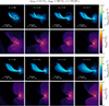 |
Fig. 1. Snapshots of TDEs of 0.6 M⊙ WDs, due to 500 M⊙ IMBHs (white points) for eight different values of impact parameter b at ∼500 s. The top two (bottom two) panels show slices of densities and temperatures for b = 0.20, 0.19, 0.18, 0.17 (b = 0.16, 0.15, 0.12, 0.10), respectively. As b decreases, the ejecta are more spread out and increasingly unlike a standard TDE, indicating runaway nuclear burning (e.g., the case of b = 0.10). The masses of the unbound ejecta are shown in Table 1. |
Masses munbound, mass fractions funbound, kinetic energies EK,unbound, and nickel masses m (56Ni) of the unbound ejecta of WD TDEs for different b values (mWD = 0.6 M⊙).
3.2. Nuclear abundances
As encounters become stronger, i.e., as b decreases, maximum temperatures of the tidally-compressed degenerate material increase, resulting in greater amounts of 12C and 16O being converted to heavier isotopes. Runaway fusion occurs at periapsis passage, when the tidal compression is strongest. Thus, the timescale of nuclear fusion is comparable to tdyn = 2.7 s (see also Section 2). After this brief period, no fusion occurs, and nuclear fractions stabilize.
Figure 2 provides a comprehensive table of nuclear mass fractions of the WD ejecta after periapsis passage. Only the isotopes with abundances > 10−4 are listed here. The trends of some important isotopes are as follows:
-
12C and 16O fractions range from ∼50% when b = 0.20 (virtually no fusion) to ∼1 − 2% when b = 0.10. More than half of their initial fractions are depleted when b = 0.16 − 0.17.
-
28Si and 32S fractions peak at ∼6 − 9% when b = 0.16 − 0.17 and then decrease to ∼1.5% when b = 0.10.
-
36Ar and 40Ca fractions peak at ∼2% when b = 0.16 and then decrease to < 1% when b = 0.10.
-
56Ni fractions increase from ∼1% when b = 0.19 (basically 0 when b = 0.20) to ∼82% when b = 0.10. The largest relative increase occurs in the range b = 0.16 − 0.19 when the 56Ni mass fraction increases by a factor of 40.
-
58Ni and 59Ni fractions also increase up to ∼2 − 3% when b = 0.10.
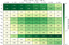 |
Fig. 2. Isotope mass fractions (those with abundances > 10−3) of the WD ejecta after periapsis passage for different values of b. As b decreases, the fractions of 12C and 16O after TDE decrease due to more nuclear burning, and the fraction of 56Ni produced increases quickly. Intermediate-mass isotopes (Ne to Ca) first increase in fraction with decreasing b, and then decrease due to more favorable conditions for massive isotope (e.g., 56Ni) production. |
As expected, deeper encounters lead to further nuclear burning due to increasingly favorable conditions. Consequently, with decreasing b, 12C and 16O fractions decrease, intermediate isotope (28Si, 32S, 36Ar, 40Ca, etc.) fractions first increase and then decrease, and 56Ni (and other massive isotopes) fraction increase. Such properties are standard of thermonuclear fusion and lead to ejecta with relative abundances between iron-group elements (IGEs), intermediate-mass elements (IMEs), and unburnt C/O that are roughly in line with SN Ia models, whether one considers Chandrasekhar mass or sub-Chandrasekhar mass WDs (see, for example, Seitenzahl et al. 2013). The main differences are the relatively lower abundances of IMEs (either material remains unburnt or tends to burn all the way to IGEs), the wider range of values for the 56Ni fraction (from as low as zero at b = 0.20 up to ∼82% at b = 0.10, which extends beyond the 56Ni fraction of 61% in Chandrasekhar mass model DDC0 or 73% of sub-Chandrasekhar mass model SCH7p0 of Blondin et al. 2017). This extreme range thus covers from explosions more typical of stripped-envelope (or perhaps ultra-stripped) SNe of Type Ic (C/O-rich debris for b = 0.19), to faint SNe Ia with a low 56Ni ejected mass (e.g., 91bg-like events; Filippenko et al. 1992a) up to the most IGE-dominated SNe Ia as inferred for 91T-like events (e.g., Filippenko et al. 1992b; Schmidt et al. 1994; Phillips et al. 2024).
Figure 3 is a collage of in-plane slices of isotope densities of 16O, 28Si, and 56Ni at ∼500 s. When b = 0.20, most of the ejecta are composed of 12C (not shown) and 16O, and the fractions of 56Ni increase with decreasing b. The onion-like structure of the ejecta is quite evident, with 56Ni, 28Si, and 16O dominating the inner, intermediate, and outer regions relative to the centers of the debris plumes. This onion-like structure also holds for other isotopes, with more massive isotopes residing in inner shells. For example, 12C, similar to 16O, is found in the outer regions; 32S, 36Ar, 40Ca, etc., as 28Si, are present in the intermediate regions; and so on. It is important to note that, since the centers of the debris plumes are not at rest but move away from the black hole (unlike standard SNe Ia that are point explosions), this stratification is not present in the radial velocity space; i.e., ejecta at all velocities are composed of material of different compositions, contrary to standard SNe Ia.
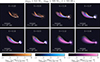 |
Fig. 3. Snapshots of slices of 16O, 28Si and 56Ni densities, respectively, similar to Figure 1. As b decreases, a higher abundance of 56Ni is produced, at the expense of 16O (and 12C), due to runaway nuclear burning. Abundances of 28Si (and other isotopes from Ne to Ca) initially increase with decreasing b, peaking around b ∼ 0.16 − 0.17, and decrease after (see also Figure 2). When nuclear burning is significant, the inner, intermediate, and outer regions of the ejecta (relative to the centers of the plumes of debris) are dominated by 56Ni, 28Si (also other intermediate isotopes), and 16O (also 12C), respectively. The transition from a standard TDE (b = 0.20) to TDE+SN is clear. |
3.3. Ejecta geometry and dynamics
A direct consequence of highly exothermic nuclear fusion reactions is the injection of internal energy into the ejecta. The ejecta spread outward and expand ballistically, as in an SN explosion. However, due to the inherent asymmetry of the WD-IMBH encounter, the geometry of the ejecta is also highly asymmetric.
Figure 4 shows polar plots of plane-projected masses within wedges of opening angle 10°, mproj,10°, unbound from the IMBHs in three perpendicular planes xy, yz, and zx at ∼500 s, for b = 0.15 with and without enabling the NRN. Changing the opening angle changes the absolute values of munbound, but not the relative differences. As a reference, the encounters take place on the xy plane with the IMBH at the center; the WD arrives from the (−x,−y) direction, periapsis approach is in the +x direction (very close to the IMBH), and the material is ejected mostly in the (−x,+y) direction. When the NRN is disabled, no nuclear reactions occur and, hence, a standard TDE, displaying tidal streams directed towards and away from the IMBH, ensues. Thus, the mass is directed outward in a thin tidal stream. On the other hand, when the NRN is enabled, the ejecta spread out more in all directions, including the +z and −z directions. However, the mass distribution is still highly asymmetric, with most of the mass being ejected in a cone of 30° about the −x direction, angled towards the +y direction.
 |
Fig. 4. Polar plots of plane-projected masses within wedges of opening angle 10°, mproj,10°, unbound from the IMBHs at ∼500 s. The solid and dashed lines represent the b = 0.15 TDE when the NRN is enabled and disabled, respectively. The three subplots represent three perpendicular planes, xy, yz, and zx, passing through the IMBHs (plot centers). The cylindrical angles are defined relative to the x, y, and z axes, respectively. Note that the values denote the sum of the projected column masses for each angle. A standard TDE ensues when the NRN is disabled, while nuclear fusion occurs when the NRN is enabled. Due to energy injected from nuclear reactions, the ejected material, in this case, spreads out more. |
Figure 5 shows similar polar plots for different values of b. The ejecta geometry when b = 0.20 is similar to when the NRN is disabled (Figure 4). As b decreases, it can be seen that the ejecta fan out not only in the +z and −z directions, but also in the xy plane.
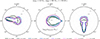 |
Fig. 5. Polar plots of mproj,10° similar to Figure 4 with the NRN enabled for different TDE b values. It is clear that the ejected material is asymmetrically distributed in all cases. As b decreases, the ejecta spread out more due to greater energy injection from nuclear fusion. This change is most drastic between b = 0.20 (standard TDE with negligible nuclear burning) and b = 0.19 (some nuclear burning). |
The ejecta expand outward from the IMBH with very high velocities of ∼0.05 c, where c is the speed of light. Figure 6 is a collage of slices, passing through the IMBH, of the b = 0.15 encounter in the xy, yz, and zx planes at ∼500 s. The arrows in each panel represent the projected radial velocities of the ejecta with respect to the IMBH in the respective planes. Almost all of the ejecta, except those bound to the IMBH, move outward ballistically. As inferred from Figures 4 and 5, most of the ejecta are contained within a cone of 30° about the −x direction. In the following sections, we focus mainly on this region.
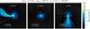 |
Fig. 6. Snapshots of slices of density of a WD TDE with b = 0.15 at ∼500 s. The three panels represent slices, passing through the IMBH, in the xy (left), yz (center), and zx (right) planes. The arrows represent the plane-projected radial velocities of the debris with respect to the IMBH at the plot centers. An arrow as long as the panel side length represents the speed of light. The dashed lines in the left and right columns represent a cone of 30° oriented along the −x direction – this cone contains almost all of the debris from the TDE and the subsequent SN. |
In a standard TDE where the initial orbit of the star is assumed to be parabolic, ∼50% of the initial mass is bound to the BH, and ∼50% becomes unbound (e.g., Hills 1988; Rees 1988). However, extra energy from nuclear fusion results in larger fractions of mass becoming unbound and escaping with large velocities. Table 1 quantifies the dynamics of the unbound ejecta: the masses munbound, mass fractions funbound, kinetic energies EK,unbound, and nickel masses m (56Ni). When b = 0.20, ∼56% of the initial WD becomes unbound from the IMBH, similar to a standard TDE. As b decreases, the unbound mass increases, with the b = 0.10 encounter resulting in ∼85% of the initial WD mass becoming unbound. Therefore, the kinetic energies of the ejecta also increase with decreasing b, from ∼1051 erg when b = 0.20 to ∼1.6 × 1051 erg when b = 0.10. The presented quantities are calculated at 150 − 200 s after periapsis. At later times (t ≳ 300 s), EK,unbound notably increase in the cases with little to no nuclear fusion and most fallback of material, i.e., b = 0.20 and b = 0.19, due to the formation of an evacuated region with very high velocities3 close to the IMBH (clearly seen in the top-left panel of Figure 1, the b = 0.20 encounter). These high-velocity outflows are far less prominent in lower-b encounters, where nuclear fusion causes the ejecta to expand and re-pressurize any evacuated region, resulting in little change to their EK,unbound. This phenomenon is illustrated in Figure B.1, which shows the kinetic energy contribution from unbound material in different density ranges at ∼200 s and ∼500 s, for different values of b. The evolution of the ejecta up to 1 d using 1D radiation hydrodynamics (see Section 4) shows fallback of some of the unbound material to the IMBH. Finally, the nickel masses increase with decreasing b, with almost 0.5 M⊙ of 56Ni being ejected when b = 0.10.
4. Radiative transfer calculations for SNe Ia from TDEs
This section describes an exploration for the radiative-transfer modeling of the debris obtained in the AREPO simulations described above. The task is challenging because of the highly asymmetric distribution of the dense, 56Ni-rich material unbound in these TDEs. We present a simplified approach that captures some of the salient features of such TDEs but misses a few (detailed below). Nonetheless, it complements previous work on the radiative-transfer modeling of such asymmetric debris that was presented in MacLeod et al. (2016). More specifically, we covered a wider range of configurations, had a more detailed ejecta composition (thanks to a more complete NRN), extended the simulations to the nebular phase (∼100 d), and handled nonlocal-thermodynamic equilibrium more accurately. However, our treatment of asymmetry was approximate and simplistic because we did not tackle the full 3D problem, as can be done with a Monte Carlo approach. Instead, we used a combination of 1D and 2D, grid-based codes for the radiative transfer to capture the strong asymmetry of WD TDEs and predict the associated observables.
As shown in Figure 1, there is a density contrast of order 104 or more between the material ejected along the direction −x and the material that surrounds it. Our approach is to approximate this complex geometry of the ejecta (this elongated plume) as being 2D and axisymmetric, with the bulk of the mass ejected along a cone with its tip at the center of the BH. We decided to model the radiative transfer for this 2D configuration using the 2D, steady-state polarized radiative-transfer code LONG_POL (Hillier 1994, 1996), upgraded to model supernova (SN) ejecta (Dessart & Hillier 2011) and applied to Type II-Plateau SNe (Dessart et al. 2021) as well as interacting, Type IIn SNe (Dessart et al. 2025). The 2D code LONG_POL requires inputs from the 1D nonlocal thermodynamic equilibrium time-dependent radiative transfer code CMFGEN (Hillier & Miller 1998; Hillier & Dessart 2012), which itself requires as input an ejecta in homologous expansion. Given that there is essentially no observation of TDEs (or SNe) at very early times, time-dependent CMFGEN calculations are typically started at 1 d or later.
Because the AREPO simulations were stopped at about 500 s, all debris needed to be evolved first until 1 d. In this section, we describe in detail each of these preparatory steps, providing along the way a number of results concerning the dynamical evolution of the debris as well as the predictions for the light curves and optical spectra of the 1D counterpart to the debris from the AREPO simulations (Section 4.2). We then describe the methodology of the 2D radiative-transfer calculations with LONG_POL as well as the results in Section 5.
4.1. Preparation of inputs at 1 d
For the last snapshot at ∼500 s of each AREPO simulation, we performed spherical shell-averaging around the IMBH to obtain the 1D radial profiles of density, temperature, radial velocity, and isotopic abundances of the ejecta (hence all as a function of distance from the IMBH). Only the cells unbound from the IMBH (i.e., those with a positive total energy, which sums the kinetic, potential, and internal energy parts) were included in the calculation. In addition, since almost all ejecta are in a cone of 30° oriented along the −x direction (see Figure 6), we only calculated the shell-averages for cells within the cone.
The angular average of the distribution of material along the −x direction at ∼500 s was remapped into the radiation-hydrodynamics code V1D (Livne 1993; Dessart et al. 2010). In the process, we averaged the composition within each radial slice, hence losing the heterogeneous composition present in the 3D debris. As shown in Figure 3, unburnt material (i.e., C and O) is located in a shell outside the metal-rich, internal regions of the asymmetric ejecta, and thus stands apart from explosive ashes traced by, for example, 56Ni. However, because of the peculiar geometry, this unburnt material is present at all ejecta velocities, from the slower-moving regions close to the BH and around the plume all the way out to the largest velocities away from the BH. In contrast, unburnt material in standard, quasispherical (i.e., relative to SNe Ia TDEs) Type Ia SN ejecta survives only in the outermost ejecta layers, and thus only at the largest velocities. This different chemical stratification is a fundamental difference between the ejecta of standard SNe Ia and those from WD-TDEs.
These spherically-averaged debris were then evolved until about 1 d. The b = 0.20 case was excluded from the sample because it contains no 56Ni. This evolution was computed in the same manner as for core-collapse SN ejecta, that is, by including gravity (here from a central 500 M⊙ BH rather than a ∼1.5 M⊙ neutron star) and by allowing for radioactive decay from unstable nuclei (primarily from 56Ni). We ignored any power injection from the BH (e.g., as from fallback accretion) – the BH was assumed to be dormant throughout. This preparatory step also neglects any multi-dimensional effect – the material along the considered direction behaves as if its spatial distribution were spherically symmetric. To attenuate the large composition gradients in the debris (in particular the sharp jumps that develop in the inner ejecta), we smoothed the composition at 1000 s with a boxcar width of 0.05 M⊙. Because of the assumption of spherical symmetry, all ejecta masses (total and isotopic) are typically 10-20 times larger than in the original 3D AREPO simulation counterpart.
In contrast to Type Ia SN ejecta, which reach homologous expansion after a few tens of seconds, a SN Ia TDE is influenced by the gravitational pull of the central (here of 500 M⊙) BH, and the ejecta are still far from reaching homologous expansion at the end of our simulations. Consequently, even though the input from AREPO was truncated at small radii to include only unbound material at ∼500 s, we found that some material falls back into the BH during the subsequent evolution. As illustrated for the b = 0.15 case in the top panel of Figure 7, there are two visible effects. First, about a tenth of a solar mass falls back within a few hours after the start of the simulation, which creates a central “hole” in the debris since no material is ejected with velocities below about 3000 km s−1. Second, the velocities of the debris layers above drop by up to a factor of two during this expansion out of the gravitational potential well, reaching homologous expansion (V ∝ r) only after several hours. Further out in the debris, this pull is weaker, and the material follows a ballistic trajectory earlier. The inner velocity hole varies in size within our model set (bottom panel of Figure 7). It is the largest in the model with the lowest 56Ni mass, which also has the lowest kinetic energy and the highest density in the inner debris at 500 s. In other models, the jump varies in size and extent, with no clear monotonic relation to 56Ni mass.
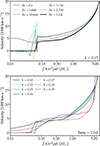 |
Fig. 7. Velocity versus “spherical” mass (i.e., ∫4πr2ρdr) obtained with the radiation-hydrodynamics code V1Dfor the b = 0.15 case at multiple times up to 1 d (top) and the full model set at 1 d (bottom). A velocity hole is observed in the unbound debris below ∼3000 km s−1 due to fallback of material. |
Physically, this fallback is related to the large escape speed of a few 1000 km s−1 for a 500 M⊙ BH even at large radii of 107 − 108 km. Observationally, it is an important signature since it not only connects to the BH mass but would also have a spectroscopic signature since no spectral line emission or absorption can arise from these essentially void inner regions.
4.2. Results for the 1D-equivalent models computed with CMFGEN
The results from V1D were mapped into CMFGEN about one day after the disruption and explosion of the white dwarf. We proceeded using the standard technique, as described, for example, for similar simulations of SNe Ia in Blondin et al. (2023), in particular, for the updated atomic data and model atoms that we adopted verbatim from that work. Homologous expansion was strictly enforced. We accounted for important species, including He, C, N, O, Ne, Na, Mg, Al, Si, S, Ar, Ca, Sc, Ti, V, Cr, Mn, Fe, Co, and Ni. We allowed only for the decay of 56Ni and 56Co since 56Ni vastly dominates in both decay power and abundance compared to any other unstable isotope produced in those explosions and for the times considered here.
Figure 8 shows the initial composition profile for He, O, Si, Ca, and Ni at the start of the CMFGEN simulation at 1 d for models b = 0.10 (i.e., the model with the highest 56Ni mass), b = 0.15 (i.e., an intermediate case), and b = 0.19 (i.e., the model with the lowest, though nonzero 56Ni mass), as well as the density profile for the full set of models. The central cavity, bounded from above by a narrow dense shell up to 100 times denser, is visible in the density profiles. The composition profiles show little chemical stratification (this effect is artificially enhanced by the adopted spherical averaging) so that all elements are typically present with at least a mass fraction of 1% at any location in the ejecta – this arises from the peculiar chemical segregation in SNe Ia TDEs (see earlier discussion and Figure 3). This will matter when analyzing the spectral information since a given element may emit or absorb radiation and thus contribute to the local cooling at any location in the debris.
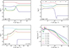 |
Fig. 8. Composition profiles for models b = 0.10 (top left), b = 0.15 (top right), and b = 0.19 (bottom left), as well as density profiles for the whole model set (bottom right), all at ∼1 d and used as initial conditions for the 1D radiative transfer calculations. We show a few of the dominant species in the ejecta. The Ni profile accounts for radioactive decay (essentially all Ni is due to 56Ni). All elements are present at different radial velocities of the ejecta. |
Because of the 1D modeling of the highly-asymmetric 3D debris, the (spherically-extrapolated) ejecta energy and masses in the 1D CMFGEN models are much greater than typically encountered in SNe Ia. The 1D model corresponding to b = 0.10 has an ejecta mass of 7.19 M⊙, a kinetic energy of 1.41 × 1052 erg, and a 56Ni mass of 6.11 M⊙. At the opposite end, the b = 0.19 model has a similar ejecta mass of 5.16 M⊙, a lower kinetic energy of 3.6 × 1051 erg, and a much lower 56Ni mass of 0.085 M⊙ – this spherical mass is typical of core-collapse SNe and should produce a peak luminosity comparable to what is observed in SNe Ibc. In contrast, the b = 0.10 model should produce a large luminosity.
The left panel of Figure 9 shows the bolometric light curves for the CMFGEN simulations of the 1D counterpart of the 3D AREPO simulations for the b = 0.10, 0.12, 0.15, 0.16, 0.17, 0.18, and 0.19 models (model b = 0.20 was not considered because it is 56Ni free). Our model set covers rise times of ∼14 d to ∼23 d to a bolometric maximum of 1.8 × 1042 erg s−1 to 8.3 × 1043 erg s−1. All simulations up to the last time of 45.2 d were computed with the time-dependent solver in CMFGEN. An additional epoch was computed, but in steady state at 100 d, where the conditions are nebular. At that time, the light curve shows a flattening because an increased fraction of the decay power arises from locally absorbed positrons from the decay of 56Co.
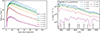 |
Fig. 9. Radiative properties of the 1D counterpart calculated with CMFGEN and based on the 3D models computed with AREPO. We show the bolometric light curves (left) and the maximum-light optical spectra for our model set (right). Closer encounters (e.g., b = 0.10) are brighter and show stronger Fe III lines in their spectra, while wider encounters (e.g., b = 0.19) are dimmer and show stronger O I, Si II, and Ca II lines in their spectra. |
The optical spectra at bolometric maximum (right panel of Figure 9 are naturally ordered in decreasing flux from b = 0.10 to b = 0.19, all showing broad P-Cygni type line profile morphologies. The b = 0.10 model and analogs at high 56Ni mass exhibit a dominance of Fe III lines (e.g., at 4419.6 Å and 5156.1 Å, but there are a myriad of lines, including contributions from Co III at that time) whereas the b = 0.19 model and analogs at low 56Ni mass exhibit a dominance of lines from intermediate mass elements with O I (e.g., at 7771.4 Å), Si II (e.g., at 6355.2 Å), and Ca II (e.g., the near-infrared triplet that spreads over the 8000 − 9000 Å region). In between, our models show a mixture of both sets of lines and produce more complex line profiles, for example, with lines of Si II and Fe II–Fe III around 6500 Å.
The spectral evolution computed with CMFGEN for the b = 0.15, 0.17, 0.18, and 0.19 models at 1.5, 5, 10, 20 and 45 d is shown in Figure 10. The b = 0.10 and b = 0.12 models with larger 56Ni masses than the b = 0.15 model have a similar spectral morphology and a global offset in flux (thus not shown). Most of the diversity occurs at the lower end of the 56Ni distribution where the contribution from IMEs strengthens. This is made more evident in Figure 11 where all models computed with CMFGEN are shown at 100 d. The difference at this later time is the additional presence of forbidden lines, primarily of [Co III] 5888.5 Å and [Fe III] 4658.0 Å in models with a high 56Ni mass whereas [O I] 6316.0 Å and [Ca II] 7307.7 Å dominate in our models with modest amounts of 56Ni. Hence, this grid effectively covers from SNe Ia ejecta entirely dominated by IGEs similar to 91T-like events (for a review, see Phillips et al. 2024), to standard Type Ia SN ejecta (e.g., SN 2002bo; Benetti et al. 2004; Blondin et al. 2015), and down to ejecta that are more similar in composition to Type Ic SNe (C and O dominated with little 56Ni; e.g., Nomoto et al. 1994).
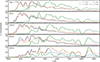 |
Fig. 10. Montage of spectra at 1.5, 5, 10, 20, and 45 d for the 1D models when b = 0.15, 0.17, 0.18, and 0.19. These epochs cover the high-brightness optically thick phase. For line identifications, see the other figures. |
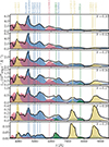 |
Fig. 11. Montage of spectra for the 1D-equivalent of the 3D models computed with CMFGEN at 100 d after the tidal disruption. A color coding is used to differentiate the emission from O, Ca, Co, and Fe, which dominate at that late time. The spectra of closer encounters with larger 56Ni masses (e.g., b = 0.10) are dominated by Co III and Fe III lines, while those of wider encounters with lower 56Ni masses (e.g., b = 0.19) are dominated by O I and Ca II lines. |
This evolution in time and relative to 56Ni mass is similar to what has been shown in numerous other studies for the explosion of both Chandrasekhar and sub-Chandrasekhar white dwarfs (e.g., Hoeflich & Khokhlov 1996; Sim et al. 2010; Blondin et al. 2013; Pakmor et al. 2013; Dessart et al. 2014) and does not warrant further discussion. It is done here to set the stage for the later discussion on the 2D simulations.
5. Results from 2D radiative-transfer calculations
The 1D simulations presented in the preceding section were post-processed at multiple epochs with the 2D, steady-state polarized radiative-transfer code LONG_POL. In practice, the 2D code reads the 1D wavelength-dependent total (line and continuum) opacities χ, emissivities η, and electron densities Ne versus the velocities output by the CMFGEN calculations and remaps these onto the 2D, spherical polar grid of LONG_POL. The asymmetry of the 3D AREPO simulations was encoded in LONG_POL through a latitudinal scaling of χ, η, and Ne. Below a polar angle of θ0 (relative to the axis of the cone at θ = 0 deg), this scaling factor was set to unity, whereas beyond it was set to vary as α + (1 − α)exp(−β2), where β = (θ − θ0)/Δθ. To reflect the asymmetry of the 3D debris, we adopted α = 10−8, θ0 = 15deg, and Δθ = 10deg. We found that the value of α had to be very low in order to quench the contribution from the material surrounding the unbound ejecta, particularly at early times when the debris is still dense and optically thick. Figure C.1 illustrates this latitudinal scaling.
Obviously, this treatment of the asymmetry is very rough. When assuming spherical symmetry, the deeper ejecta layers are not only denser, which leads to a smaller photon mean free path, but they are also enshrouded within the overlying ejecta layers, which may contribute a significant optical depth. This affects the propagation of both γ-rays (i.e., from radioactive decay emission) and low-energy photons. When one allows for asymmetry (whether truly in 3D or in the approximate morphology in 2D), the deeper layers are equally dense as in the 1D case, but they are no longer enshrouded. This holds for the sides of the “cone”, or for the innermost layers which are effectively bare. In our post-treatment of the 1D CMFGEN simulations with LONG_POL, we ignored this aspect and thus overestimate the temperature and ionization of these deeper layers. This means that we overestimate the emissivity of the deeper layers, which affects all observables for viewing angles away from θ = 0deg. More specifically, we overestimate the brightness (a global shift in all bands), the color (predictions will be overly blue in the optical), and the ionization (we may predict emission from twice-ionized species, whereas once-ionized species may dominate). This issue is, however, not as bad as it may seem since the inner ejecta are 105 times denser than the outer, fast-moving ejecta regions. Thus, even if the inner ejecta regions are bare, the mean-free-path of both low- and high-energy photons is small, and radiation is considerably more trapped in the inner ejecta regions than in the outer ejecta regions. A more suitable approach would be to solve the full radiative transfer of low- and high-energy photons in 3D, as done in MacLeod et al. (2016) – this is deferred to future work.
The immediate difference that results from this 2D treatment is that the ejecta and isotopic yields are now commensurate with those from the 3D simulations (i.e., the 2D ejecta volume is reduced by a factor of about 20 compared to the spherical case). In 2D, the unbound material in the b = 0.10 (b = 0.19) model now has a total mass of 0.34 M⊙ (0.24 M⊙), compared to ejecta masses in the 3D AREPO simulations of 0.51 M⊙ (0.34 M⊙) and of 7.11 M⊙ (5.14 M⊙) compared to the spherical counterparts of the preceding section. Consequently, the light curves are now more comparable with those of Type Ia SNe. Since we did not aim to reproduce the 3D debris masses exactly, we applied the same latitudinal scaling (α, θ0, and Δθ parameters) for all simulations.
Figure 12 shows the B-band light curves computed for a variety of models and viewing angles with LONG_POL (for comparison, the spherical counterparts obtained with CMFGEN are included). The overall offset with the 1D results is 2 − 3 mag due to the reduced 56Ni mass. The predicted brightness is greater for viewing angles away from θ = 0deg. This is qualitatively similar to the results of MacLeod et al. (2016), although they obtained a larger offset of about 2 mag for their model with 0.13 M⊙ of 56Ni (equivalent to the b = 0.17 model here). This dependency on viewing angle results from a combination of effects. One is the change in the size of the emitting surface seen by the observer (i.e., greater for viewing angles closer to 90deg). Another is the observation of hotter, inner ejecta regions for viewing angles away from θ = 0deg. In our work, the results for the photometry are impacted by the adoption of the emissivity from the 1D CMFGEN models, which underestimates photon escape (and thus cooling) from the inner ejecta layers. Interestingly, the photometric offset is still present at 100 d when conditions are nebular (the total inward-integrated radial Rosseland-mean optical depth is 0.9 in the model b = 0.16 at 100 d).
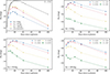 |
Fig. 12. Photometric properties of SNe Ia TDE models computed with LONG_POL. Top left: B-band light curve of the b = 0.16 model for viewing angles of 0, 90, and 180deg. We also overplot the CMFGEN results (assuming spherical symmetry). Other panels: Same as top left, but comparing different models for a given viewing angle. The B-band brightness is greater for closer encounters and viewing angles away from 0deg. |
Overall, and not surprisingly, these photometric properties are comparable to those of SNe Ia, be it observed ones or models thereof, that are characterized by the same range in 56Ni mass. With the 2D simulations, only a limited spectral range was modeled, and thus no bolometric luminosity can be recovered from the LONG_POL calculations. We compared the B-band magnitudes instead. In the set of Chandrasekhar mass and sub-Chandrasekhar mass models of Blondin et al. (2017, these simulations are a good set to compare to since they match for the most part the width-luminosity relation, as well as the photometric and spectral evolution, of SNe Ia), the peak B-band magnitudes span the rough range from −17 to −19 mag for 56Ni masses in the range ∼0.1 − 0.5 M⊙, with corresponding B-band rise times of ∼17 d. Our set extends to much lower peak B-band magnitudes because it reaches down to very low 56Ni masses (e.g., 0.007 M⊙ with model b = 0.19). Our model rise times cluster around 20 d, thus slightly larger but in rough agreement with theirs. A possible reason for this systematic shift may be the slower expansion of the ejecta that arises from the gravitational pull by the central BH, thus leading to a slightly larger ejecta diffusion time relative to standard SNe Ia. What is unique with SN-TDEs is the strong viewing angle dependence of these ejecta, leading to a variation in brightness for the same 56Ni mass.
Figure 13 shows the spectral evolution from about 5 to 40 d for the b = 0.16 model for a viewing angle of 0, 90, and 180deg. This covers most of the photospheric phase and thus straddles the time of bolometric maximum. Hence, the spectra shift upwards until about 20 d before shifting downwards towards a lower power. For a viewing angle of 0deg, one observes the debris along the direction of expansion. At the earliest time, the spectra show much structure and rapidly change with wavelength. This arises from the fact that we are essentially observing the troughs of what would in 1D appear as a fully developed P-Cygni profile with both absorption and a broad emission (see Figure 9 or Figure 10) – only the absorption part is essentially present for that viewing angle because the debris are confined within a narrow cone pointing towards the observer. As time progresses, the photosphere recedes in the ejecta, lines become narrower but still exhibit a systematic blueshift.
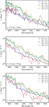 |
Fig. 13. Spectral evolution in the optical for the 2D b = 0.16 model and for viewing angles of 0deg (top), 90deg (middle), and 180deg (bottom). The spectra change rapidly with wavelength at earlier times and lines become narrower with time. The spectral lines at 0deg and 180deg are blueshifted and redshifted, respectively (most evident at later times). |
For a 90deg viewing angle, the ejecta expansion is perpendicular to the line of sight. At once, the observer captures emission from all ejecta depths but with a smaller range in projected velocity due to the finite angular extent of the cone of ∼30deg seen at a 90deg angle.
For a 180deg viewing angle, the ejecta expansion is now away along the line of sight, and the emission arises preferentially from the inner, hot, and dense inner ejecta layers. All line emission and absorptions are consequently redshifted, although this is not easily noticed because of the myriad of contributing lines and their overlap. This Doppler shift is, however, evident when one compares one epoch for the three viewing angles. For example, a vertical line (as can be created by using the edge of the computer screen), clearly stands redward, along the center, or blueward of the Ca II NIR emission for viewing angles of 0, 90, or 180deg.
Figure 14 illustrates the spectral properties of the b = 0.10, 0.16, and 0.19 models at bolometric maximum, but comparing the properties for the three viewing angles of 0, 90, and 180deg in each panel. The flux is usually greater for 90 and 180deg angles since they reveal the inner, hotter ejecta layers, although this can be mitigated by the chemical stratification (e.g., if 56Ni is present throughout the ejecta as in the b = 0.10 model or more confined to the inner ejecta as in the b = 0.19 model). Insets in the three panels of Figure 14 show a zoom-in on the flux in Doppler velocity centered on the strong transitions of Fe II at 5169 Å or O I at 7773.4 Å. There is evidently a shift from blue to red as the viewing angle increases, although even in this narrower spectral range, additional transitions contribute.
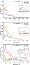 |
Fig. 14. Optical spectra for models b = 0.10 (top), b = 0.16 (middle), and b = 0.19 (bottom) at the time of bolometric maximum (of the 1D model counterpart) for viewing angles of 0, 90, and 180deg. The zoomed-in panels show wavelength shifts in the spectral lines that depend on viewing angle. |
Figure 15 is a counterpart of Figure 14 but now at 100 d. At nebular conditions, the spectrum is dominated by a few strong emission lines, including gaps with no emission beyond 5500 Å, essentially associated with regions devoid of Fe II lines. Here too, some insets are used to reveal the wavelength shifts in some strong emission lines, using as diagnostics the air wavelength of [Fe III] 4658 Å, the gf-weighted4 mean wavelength of the Ca II NIR triplet, or that of [Ca II] λλ 7291, 7323.
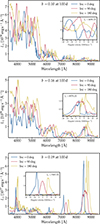 |
Fig. 15. Optical spectra for models b = 0.10 (top), b = 0.16 (middle), and b = 0.19 (bottom) at 100 d and for viewing angles of 0, 90, and 180deg. The zoomed-in panels show wavelength shifts in the spectral lines that depend on viewing angle. |
The projected velocity of the emission is shifted by 5000 − 10 000 km s−1 as the viewing angle changes from 0 to 180deg. In addition, we clearly see the absence of emission from within 5000 km s−1 for viewing angles of 0 and 180deg, which arises from the lack of material below about 5000 km s−1 in all the SNe Ia TDEs simulated here. This is directly visible in the b = 0.19 model, but harder to identify in the b = 0.16 model in which we used the Ca II NIR triplet (each component at 8498.0 Å, 8542.1 Å, and 8662.1 Å is optically thick and affects the whole triplet out to many 1000 km s−1) or the b = 0.10 model because 56Ni is originally present throughout the ejecta (i.e., a large range of depths contribute line emission).
6. Discussion and conclusions
We explored close TDEs of C/O WDs due to IMBHs using the 3D hydrodynamics code AREPO, including an on-the-fly NRN with 55-isotopes, and the 1D and 2D radiative transfer codes CMFGEN and LONG_POL, respectively. Setting the masses of the WD and the IMBH to 0.6 M⊙ and 500 M⊙, respectively, we studied the effect of the scaled encounter impact parameters b = rp/rt (ranging from 0.10 to 0.20) on their outcomes. We ran the 3D hydrodynamics simulations until ∼500 s following periapsis passage, after which we employed the 1D radiation hydrodynamics code V1D to run them further until homologous expansion of the ejecta was attained at 1 d. These data were then input into the 1D and 2D radiation transfer codes to obtain their light curves and spectra in the photospheric (≲40 d) and nebular phases (∼100 d).
The most striking result of our WD TDE simulations is the strong dependence of the chemical composition and morphology of the ejecta on b. Stronger encounters (lower b) yield higher peak temperatures in the tidally compressed WDs, resulting in increased nuclear burning of 12C and 16O into heavier isotopes. Consequently, while a wider encounter (e.g., b = 0.20) leads to a standard full TDE (the WD is completely destroyed) with negligible burning, a closer encounter (e.g., b = 0.10) results in an SN 1a TDE where a full TDE is supplemented by runaway nuclear burning. The fractions of 56Ni produced in such SNe Ia TDEs range from 1% when b = 0.19 to 82% when b = 0.10. We note that the specific case of b = 0.20 in Rosswog et al. (2009)5 resulted in a SN explosion, while it is akin to a standard TDE with negligible nuclear burning in our simulations. This can be attributed to their relatively low resolution of ∼5 × 10⁵ SPH particles constituting their WD, compared to our 6 × 10⁶ cells. During our resolution tests, we observed that lower-resolution simulations had higher rates of nuclear fusion (see also Section 2), likely due to the larger volumes of cells where ignition occurs.
Due to the energy injected into the ejecta from nuclear fusion reactions, the debris material spreads out more in SNe Ia TDEs compared to the thin tidal streams of standard TDEs. Thus, while ∼55% of WD material is unbound when b = 0.20 (similar to a standard TDE), ∼85% of WD is unbound when b = 0.10 (significant nuclear burning). Moreover, due to the inherent asymmetry of the WD-IMBH encounter, most of the ejecta are present within a cone of ∼30%, resulting in very asymmetric SN explosions. We expect a similar dependence of nuclear burning rates on b for different IMBH masses, although the exact rates and, consequently, massive isotope fractions would vary due to differences in tidal compression and effects of general relativity. Altering the WD masses (and hence their compositions), on the other hand, can lead to distinct outcomes because nuclear reactions in He WDs (0.15 M⊙ ≲ mWD ≲ 0.45 M⊙; e.g., Althaus et al. 2013), O/Ne WDs (1.05 M⊙ ≲ mWD ≲ 1.35 M⊙; e.g., Doherty et al. 2015) or even C/O WDs of different masses (0.45 M⊙ ≲ mWD ≲ 1.05 M⊙; e.g., Althaus et al. 2010) would play out quite differently. We leave these for future studies.
SNe Ia TDEs are most dramatically distinct from garden-variety SNe Ia in the extreme asymmetry of the debris and the presence of a central BH. Even if assumed dormant, the gravitational pull on the ejecta extends the dynamical phase (i.e., the debris moves ballistically only after a number of hours) and leads to a fallback that arves the inner ejecta below a few 1000 km s−1. The debris asymmetry also leads to a dependence of brightness and colors with viewing angles, although this also depends on the 56Ni mass and the chemical stratification. The most striking spectral signature of SNe Ia TDEs, best visible at nebular times, is the large velocity shifts of emission lines for viewing angles away from 90deg, which arise from the strong ejecta asymmetry. This shift is aggravated by the cavity in the inner ejecta, resulting in a large displacement of the line emission (i.e., both a skewness and a shift of line emission). Interestingly, this has been observed in a fast-blue optical transient with systematically blueshifted and displaced H I emission lines (Gutiérrez et al. 2024) – this event was interpreted as the TDE of an unevolved, low-mass star by an IMBH.
In this work, we have held back from making a direct comparison of the observables from the radiative-transfer calculations and the current observed dataset of SNe Ia. One reason is that we are likely still awaiting a firm observation of an SN Ia TDE (see, however, Li et al. 2025; Eyles-Ferris et al. 2026). This work is also based on the TDE of a 0.6 M⊙ C/O-WD, which is a very small mass relative to that inferred for an SN Ia (for example, such a light WD makes hardly any 56Ni in the single- or double-degenerate scenario; see, for example, Morán-Fraile et al. 2024). Another is the inconsistency in our approach for the 2D radiative transfer and the difficulty in evaluating the associated uncertainty in the predictions. While qualitatively sound, we expect systematic quantitative offsets at all photospheric epochs. At nebular times, our method and its predictions are more robust. Still, our enforcement of homogeneity within radial shells when computing both the 1D and 2D radiative transfer compromises the accuracy of the prediction. The reason is that such an enforced mixing alters the relative strength of coolants in the ejecta and thus the strength of spectral emission lines (Fransson & Chevalier 1989; Dessart & Hillier 2020). This should have little impact in models with a high 56Ni mass fraction (e.g., models with b ≥ 0.15), but it is responsible for the weakness of the [O I] λλ 6300, 6364 emission in the b = 0.19 model at 100 d (see bottom row of Figure 15).
Future improvements will require using a better description of the spatial distribution of radioactive decay power within the debris, as well as the viewing angle dependence of the luminosity. Such multidimensional constraints could be computed using SEDONA (Kasen et al. 2006; as in MacLeod et al. 2016), feeding such constraints (e.g., the viewing-angle dependent energy deposition from radioactive decay or the viewing angle dependent bolometric luminosity) as inputs for the radiative transfer calculation with CMFGEN and LONG_POL, as done for the simulations of 2D double detonations in white dwarfs (Boos et al. 2025).
Acknowledgments
PV thanks Bart Ripperda and Norman Murray for providing access to their computational time on Compute Canada’s Niagara cluster. PV thanks CITA for access to the Sunnyvale cluster. LD acknowledges support from the ESO Scientific Visitor Program for a visit to ESO-Garching during the summer of 2025. LD acknowledges access to the HPC resources of TGCC under the allocation 2024 – A0170410554 on Irene-Rome made by GENCI, France. PV and LD contributed equally to the paper, with them conducting, analyzing, and writing the hydrodynamics simulations and the radiative transfer calculations, respectively. All authors contributed to the project planning, analysis, and writing.
References
- Althaus, L. G., Córsico, A. H., Isern, J., & García-Berro, E. 2010, A&ARv, 18, 471 [NASA ADS] [CrossRef] [Google Scholar]
- Althaus, L. G., Miller Bertolami, M. M., & Córsico, A. H. 2013, A&A, 557, A19 [NASA ADS] [CrossRef] [EDP Sciences] [Google Scholar]
- Benetti, S., Meikle, P., Stehle, M., et al. 2004, MNRAS, 348, 261 [CrossRef] [Google Scholar]
- Blondin, S., Dessart, L., Hillier, D. J., & Khokhlov, A. M. 2013, MNRAS, 429, 2127 [NASA ADS] [CrossRef] [Google Scholar]
- Blondin, S., Dessart, L., & Hillier, D. J. 2015, MNRAS, 448, 2766 [NASA ADS] [CrossRef] [Google Scholar]
- Blondin, S., Dessart, L., Hillier, D. J., & Khokhlov, A. M. 2017, MNRAS, 470, 157 [Google Scholar]
- Blondin, S., Dessart, L., Hillier, D. J., Ramsbottom, C. A., & Storey, P. J. 2023, A&A, 678, A170 [NASA ADS] [CrossRef] [EDP Sciences] [Google Scholar]
- Boos, S. J., Dessart, L., Townsley, D. M., & Shen, K. J. 2025, ApJ, 987, 54 [Google Scholar]
- Bricman, K., & Gomboc, A. 2020, ApJ, 890, 73 [NASA ADS] [CrossRef] [Google Scholar]
- Chang, J. N. Y., Dai, L., Pfister, H., Kar Chowdhury, R., & Natarajan, P. 2025, ApJ, 980, L22 [Google Scholar]
- Clausen, D., & Eracleous, M. 2011, ApJ, 726, 34 [Google Scholar]
- Cyburt, R. H., Amthor, A. M., Ferguson, R., et al. 2010, ApJS, 189, 240 [NASA ADS] [CrossRef] [Google Scholar]
- Dessart, L., & Hillier, D. J. 2011, MNRAS, 415, 3497 [Google Scholar]
- Dessart, L., & Hillier, D. J. 2020, A&A, 642, A33 [NASA ADS] [CrossRef] [EDP Sciences] [Google Scholar]
- Dessart, L., Livne, E., & Waldman, R. 2010, MNRAS, 405, 2113 [NASA ADS] [Google Scholar]
- Dessart, L., Blondin, S., Hillier, D. J., & Khokhlov, A. 2014, MNRAS, 441, 532 [NASA ADS] [CrossRef] [Google Scholar]
- Dessart, L., Leonard, D. C., Hillier, D. J., & Pignata, G. 2021, A&A, 651, A19 [NASA ADS] [CrossRef] [EDP Sciences] [Google Scholar]
- Dessart, L., Leonard, D. C., Vasylyev, S. S., & Hillier, D. J. 2025, A&A, 696, L12 [NASA ADS] [CrossRef] [EDP Sciences] [Google Scholar]
- Doherty, C. L., Gil-Pons, P., Siess, L., Lattanzio, J. C., & Lau, H. H. B. 2015, MNRAS, 446, 2599 [Google Scholar]
- Eyles-Ferris, R. A. J., King, A., Starling, R. L. C., et al. 2026, MNRAS, 546, stag005 [Google Scholar]
- Filippenko, A. V., Richmond, M. W., Branch, D., et al. 1992a, AJ, 104, 1543 [NASA ADS] [CrossRef] [Google Scholar]
- Filippenko, A. V., Richmond, M. W., Matheson, T., et al. 1992b, ApJ, 384, L15 [CrossRef] [Google Scholar]
- Fransson, C., & Chevalier, R. A. 1989, ApJ, 343, 323 [NASA ADS] [CrossRef] [Google Scholar]
- Gomez, S., & Gezari, S. 2023, ApJ, 955, 46 [Google Scholar]
- Górski, K. M., Hivon, E., Banday, A. J., et al. 2005, ApJ, 622, 759 [Google Scholar]
- Greene, J. E., Strader, J., & Ho, L. C. 2020, ARA&A, 58, 257 [Google Scholar]
- Gutiérrez, C. P., Mattila, S., Lundqvist, P., et al. 2024, ApJ, 977, 162 [Google Scholar]
- Häberle, M., Neumayer, N., Seth, A., et al. 2024, Nature, 631, 285 [CrossRef] [Google Scholar]
- Hillier, D. J. 1994, A&A, 289, 492 [NASA ADS] [Google Scholar]
- Hillier, D. J. 1996, A&A, 308, 521 [NASA ADS] [Google Scholar]
- Hillier, D. J., & Dessart, L. 2012, MNRAS, 424, 252 [CrossRef] [Google Scholar]
- Hillier, D. J., & Miller, D. L. 1998, ApJ, 496, 407 [NASA ADS] [CrossRef] [Google Scholar]
- Hills, J. G. 1988, Nature, 331, 687 [Google Scholar]
- Hoeflich, P., & Khokhlov, A. 1996, ApJ, 457, 500 [CrossRef] [Google Scholar]
- Ivezić, Ž., Kahn, S. M., Tyson, J. A., et al. 2019, ApJ, 873, 111 [Google Scholar]
- Jonker, P. G., Glennie, A., Heida, M., et al. 2013, ApJ, 779, 14 [NASA ADS] [CrossRef] [Google Scholar]
- Kasen, D., Thomas, R. C., & Nugent, P. 2006, ApJ, 651, 366 [NASA ADS] [CrossRef] [Google Scholar]
- Kepler, S. O., Kleinman, S. J., Nitta, A., et al. 2007, MNRAS, 375, 1315 [NASA ADS] [CrossRef] [Google Scholar]
- Kleinman, S. J., Kepler, S. O., Koester, D., et al. 2013, ApJS, 204, 5 [NASA ADS] [CrossRef] [Google Scholar]
- Kuin, N. P. M., Wu, K., Oates, S., et al. 2019, MNRAS, 487, 2505 [NASA ADS] [CrossRef] [Google Scholar]
- Langanke, K., & Martínez-Pinedo, G. 2001, At. Data Nucl. Data Tables, 79, 1 [Google Scholar]
- Law-Smith, J., MacLeod, M., Guillochon, J., Macias, P., & Ramirez-Ruiz, E. 2017, ApJ, 841, 132 [CrossRef] [Google Scholar]
- Li, D., Zhang, W., Yang, J., et al. 2025, arXiv e-prints [arXiv:2509.25877] [Google Scholar]
- Livne, E. 1993, ApJ, 412, 634 [Google Scholar]
- MacLeod, M., Guillochon, J., Ramirez-Ruiz, E., Kasen, D., & Rosswog, S. 2016, ApJ, 819, 3 [NASA ADS] [CrossRef] [Google Scholar]
- Maguire, K., Eracleous, M., Jonker, P. G., MacLeod, M., & Rosswog, S. 2020, Space Sci. Rev., 216, 39 [NASA ADS] [CrossRef] [Google Scholar]
- Mahapatra, A., Pandey, A., Banerjee, P., & Sarkar, T. 2025, arXiv e-prints [arXiv:2508.03463] [Google Scholar]
- Mamuzic, E., Ryu, T., Suyu, S. H., et al. 2025, A&A, 701, A142 [Google Scholar]
- Morán-Fraile, J., Holas, A., Röpke, F. K., Pakmor, R., & Schneider, F. R. N. 2024, A&A, 683, A44 [NASA ADS] [CrossRef] [EDP Sciences] [Google Scholar]
- Nomoto, K., Yamaoka, H., Pols, O. R., et al. 1994, Nature, 371, 227 [NASA ADS] [CrossRef] [Google Scholar]
- Ohlmann, S. T., Röpke, F. K., Pakmor, R., & Springel, V. 2017, A&A, 599, A5 [NASA ADS] [CrossRef] [EDP Sciences] [Google Scholar]
- Pakmor, R., Edelmann, P., Röpke, F. K., & Hillebrandt, W. 2012, MNRAS, 424, 2222 [Google Scholar]
- Pakmor, R., Kromer, M., Taubenberger, S., & Springel, V. 2013, ApJ, 770, L8 [Google Scholar]
- Pakmor, R., Springel, V., Bauer, A., et al. 2016, MNRAS, 455, 1134 [Google Scholar]
- Perets, H. B., Li, Z., Lombardi, J. C., Jr., & Milcarek, S. R., Jr. 2016, ApJ, 823, 113 [NASA ADS] [CrossRef] [Google Scholar]
- Phillips, M. M., Ashall, C., Brown, P. J., et al. 2024, ApJS, 273, 16 [NASA ADS] [CrossRef] [Google Scholar]
- Rees, M. J. 1988, Nature, 333, 523 [Google Scholar]
- Rosswog, S., Ramirez-Ruiz, E., & Hix, W. R. 2009, ApJ, 695, 404 [NASA ADS] [CrossRef] [Google Scholar]
- Schmidt, B. P., Kirshner, R. P., Leibundgut, B., et al. 1994, ApJ, 434, L19 [NASA ADS] [CrossRef] [Google Scholar]
- Seitenzahl, I. R., Ciaraldi-Schoolmann, F., Röpke, F. K., et al. 2013, MNRAS, 429, 1156 [NASA ADS] [CrossRef] [Google Scholar]
- Sim, S. A., Röpke, F. K., Hillebrandt, W., et al. 2010, ApJ, 714, L52 [Google Scholar]
- Springel, V. 2005, MNRAS, 364, 1105 [Google Scholar]
- Springel, V. 2010, MNRAS, 401, 791 [Google Scholar]
- Szekerczes, K., Ryu, T., Suyu, S. H., et al. 2024, A&A, 690, A384 [Google Scholar]
- Timmes, F. X., & Swesty, F. D. 2000, ApJS, 126, 501 [NASA ADS] [CrossRef] [Google Scholar]
- Tremblay, P. E., Bergeron, P., & Gianninas, A. 2011, ApJ, 730, 128 [Google Scholar]
- Vynatheya, P., Ryu, T., Pakmor, R., de Mink, S. E., & Perets, H. B. 2024, A&A, 685, A45 [NASA ADS] [CrossRef] [EDP Sciences] [Google Scholar]
- Weinberger, R., Springel, V., & Pakmor, R. 2020, ApJS, 248, 32 [Google Scholar]
- Wevers, T., & Ryu, T. 2023, arXiv e-prints [arXiv:2310.16879] [Google Scholar]
- Ye, C. S., Fragione, G., & Perna, R. 2023, ApJ, 953, 141 [Google Scholar]
C/O ratios depend on masses and metallicities of initial stars, and impact future nuclear burning.
Since mBH ≫ mWD, this is also the same as the WD dynamical timescale rdyn, WD = (rWD3/GmWD)1/2.
Since we adopt Newtonian gravity, these velocities are likely overestimated. In reality, they would be limited by general relativity.
gf refers to the oscillator strength of an atomic transition.
Runs 8 and 9 of Table 1; same WD and IMBH masses.
Appendix A: Density profile of the white dwarf
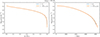 |
Fig. A.1. Density profiles of the AREPO-initialized 0.6 M⊙ WD (10−7 M⊙/cell resolution) as a function of mass (left) and radial (right) coordinates. The blue dashed and the orange solid lines denote the profiles initially (identical to 1D MESA profile) and after 10 sound-crossing times (∼127 s). The profiles overlap significantly. |
Appendix B: Kinetic energies of the unbound ejecta
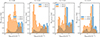 |
Fig. B.1. Kinetic energies EK,unbound of the unbound ejecta per 0.5 dex in density at ∼200 s and ∼500 s, for b ranging from 0.17 to 0.20. For b = 0.20 (and b = 0.19), EK,unbound at ∼500 s is dominated by low-density, (very) high-velocity material, and is hence larger than at ∼200 s. However, as b decreases (e.g., b = 0.17 and lower, not shown) and nuclear fusion becomes significant, there is only a slight change in EK,unbound with time owing to the decreased presence of such material. The peaks of the kinetic energies shift to lower densities with time due to the expansion of the ejecta. |
Appendix C: Latitudinal scaling in 2D radiative transfer
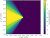 |
Fig. C.1. Latitudinal scaling used for the inputs (opacities χ, emissivities η, and electron densities Ne) to the 2D radiative transfer code LONG_POL. The dashed lines represent the boundaries of a cone of 30°. The parameters α and β set the steepness of scaling drop-off beyond the conical region and the gaussian scaling centered about the −x direction, respectively. This scaling is performed to mimic the asymmetry of the WD TDE ejecta, shown in Figure 1. |
All Tables
Masses munbound, mass fractions funbound, kinetic energies EK,unbound, and nickel masses m (56Ni) of the unbound ejecta of WD TDEs for different b values (mWD = 0.6 M⊙).
All Figures
|
Fig. 1. Snapshots of TDEs of 0.6 M⊙ WDs, due to 500 M⊙ IMBHs (white points) for eight different values of impact parameter b at ∼500 s. The top two (bottom two) panels show slices of densities and temperatures for b = 0.20, 0.19, 0.18, 0.17 (b = 0.16, 0.15, 0.12, 0.10), respectively. As b decreases, the ejecta are more spread out and increasingly unlike a standard TDE, indicating runaway nuclear burning (e.g., the case of b = 0.10). The masses of the unbound ejecta are shown in Table 1. |
| In the text | |
|
Fig. 2. Isotope mass fractions (those with abundances > 10−3) of the WD ejecta after periapsis passage for different values of b. As b decreases, the fractions of 12C and 16O after TDE decrease due to more nuclear burning, and the fraction of 56Ni produced increases quickly. Intermediate-mass isotopes (Ne to Ca) first increase in fraction with decreasing b, and then decrease due to more favorable conditions for massive isotope (e.g., 56Ni) production. |
| In the text | |
|
Fig. 3. Snapshots of slices of 16O, 28Si and 56Ni densities, respectively, similar to Figure 1. As b decreases, a higher abundance of 56Ni is produced, at the expense of 16O (and 12C), due to runaway nuclear burning. Abundances of 28Si (and other isotopes from Ne to Ca) initially increase with decreasing b, peaking around b ∼ 0.16 − 0.17, and decrease after (see also Figure 2). When nuclear burning is significant, the inner, intermediate, and outer regions of the ejecta (relative to the centers of the plumes of debris) are dominated by 56Ni, 28Si (also other intermediate isotopes), and 16O (also 12C), respectively. The transition from a standard TDE (b = 0.20) to TDE+SN is clear. |
| In the text | |
|
Fig. 4. Polar plots of plane-projected masses within wedges of opening angle 10°, mproj,10°, unbound from the IMBHs at ∼500 s. The solid and dashed lines represent the b = 0.15 TDE when the NRN is enabled and disabled, respectively. The three subplots represent three perpendicular planes, xy, yz, and zx, passing through the IMBHs (plot centers). The cylindrical angles are defined relative to the x, y, and z axes, respectively. Note that the values denote the sum of the projected column masses for each angle. A standard TDE ensues when the NRN is disabled, while nuclear fusion occurs when the NRN is enabled. Due to energy injected from nuclear reactions, the ejected material, in this case, spreads out more. |
| In the text | |
|
Fig. 5. Polar plots of mproj,10° similar to Figure 4 with the NRN enabled for different TDE b values. It is clear that the ejected material is asymmetrically distributed in all cases. As b decreases, the ejecta spread out more due to greater energy injection from nuclear fusion. This change is most drastic between b = 0.20 (standard TDE with negligible nuclear burning) and b = 0.19 (some nuclear burning). |
| In the text | |
|
Fig. 6. Snapshots of slices of density of a WD TDE with b = 0.15 at ∼500 s. The three panels represent slices, passing through the IMBH, in the xy (left), yz (center), and zx (right) planes. The arrows represent the plane-projected radial velocities of the debris with respect to the IMBH at the plot centers. An arrow as long as the panel side length represents the speed of light. The dashed lines in the left and right columns represent a cone of 30° oriented along the −x direction – this cone contains almost all of the debris from the TDE and the subsequent SN. |
| In the text | |
|
Fig. 7. Velocity versus “spherical” mass (i.e., ∫4πr2ρdr) obtained with the radiation-hydrodynamics code V1Dfor the b = 0.15 case at multiple times up to 1 d (top) and the full model set at 1 d (bottom). A velocity hole is observed in the unbound debris below ∼3000 km s−1 due to fallback of material. |
| In the text | |
|
Fig. 8. Composition profiles for models b = 0.10 (top left), b = 0.15 (top right), and b = 0.19 (bottom left), as well as density profiles for the whole model set (bottom right), all at ∼1 d and used as initial conditions for the 1D radiative transfer calculations. We show a few of the dominant species in the ejecta. The Ni profile accounts for radioactive decay (essentially all Ni is due to 56Ni). All elements are present at different radial velocities of the ejecta. |
| In the text | |
|
Fig. 9. Radiative properties of the 1D counterpart calculated with CMFGEN and based on the 3D models computed with AREPO. We show the bolometric light curves (left) and the maximum-light optical spectra for our model set (right). Closer encounters (e.g., b = 0.10) are brighter and show stronger Fe III lines in their spectra, while wider encounters (e.g., b = 0.19) are dimmer and show stronger O I, Si II, and Ca II lines in their spectra. |
| In the text | |
|
Fig. 10. Montage of spectra at 1.5, 5, 10, 20, and 45 d for the 1D models when b = 0.15, 0.17, 0.18, and 0.19. These epochs cover the high-brightness optically thick phase. For line identifications, see the other figures. |
| In the text | |
|
Fig. 11. Montage of spectra for the 1D-equivalent of the 3D models computed with CMFGEN at 100 d after the tidal disruption. A color coding is used to differentiate the emission from O, Ca, Co, and Fe, which dominate at that late time. The spectra of closer encounters with larger 56Ni masses (e.g., b = 0.10) are dominated by Co III and Fe III lines, while those of wider encounters with lower 56Ni masses (e.g., b = 0.19) are dominated by O I and Ca II lines. |
| In the text | |
|
Fig. 12. Photometric properties of SNe Ia TDE models computed with LONG_POL. Top left: B-band light curve of the b = 0.16 model for viewing angles of 0, 90, and 180deg. We also overplot the CMFGEN results (assuming spherical symmetry). Other panels: Same as top left, but comparing different models for a given viewing angle. The B-band brightness is greater for closer encounters and viewing angles away from 0deg. |
| In the text | |
|
Fig. 13. Spectral evolution in the optical for the 2D b = 0.16 model and for viewing angles of 0deg (top), 90deg (middle), and 180deg (bottom). The spectra change rapidly with wavelength at earlier times and lines become narrower with time. The spectral lines at 0deg and 180deg are blueshifted and redshifted, respectively (most evident at later times). |
| In the text | |
|
Fig. 14. Optical spectra for models b = 0.10 (top), b = 0.16 (middle), and b = 0.19 (bottom) at the time of bolometric maximum (of the 1D model counterpart) for viewing angles of 0, 90, and 180deg. The zoomed-in panels show wavelength shifts in the spectral lines that depend on viewing angle. |
| In the text | |
|
Fig. 15. Optical spectra for models b = 0.10 (top), b = 0.16 (middle), and b = 0.19 (bottom) at 100 d and for viewing angles of 0, 90, and 180deg. The zoomed-in panels show wavelength shifts in the spectral lines that depend on viewing angle. |
| In the text | |
|
Fig. A.1. Density profiles of the AREPO-initialized 0.6 M⊙ WD (10−7 M⊙/cell resolution) as a function of mass (left) and radial (right) coordinates. The blue dashed and the orange solid lines denote the profiles initially (identical to 1D MESA profile) and after 10 sound-crossing times (∼127 s). The profiles overlap significantly. |
| In the text | |
|
Fig. B.1. Kinetic energies EK,unbound of the unbound ejecta per 0.5 dex in density at ∼200 s and ∼500 s, for b ranging from 0.17 to 0.20. For b = 0.20 (and b = 0.19), EK,unbound at ∼500 s is dominated by low-density, (very) high-velocity material, and is hence larger than at ∼200 s. However, as b decreases (e.g., b = 0.17 and lower, not shown) and nuclear fusion becomes significant, there is only a slight change in EK,unbound with time owing to the decreased presence of such material. The peaks of the kinetic energies shift to lower densities with time due to the expansion of the ejecta. |
| In the text | |
|
Fig. C.1. Latitudinal scaling used for the inputs (opacities χ, emissivities η, and electron densities Ne) to the 2D radiative transfer code LONG_POL. The dashed lines represent the boundaries of a cone of 30°. The parameters α and β set the steepness of scaling drop-off beyond the conical region and the gaussian scaling centered about the −x direction, respectively. This scaling is performed to mimic the asymmetry of the WD TDE ejecta, shown in Figure 1. |
| In the text | |
Current usage metrics show cumulative count of Article Views (full-text article views including HTML views, PDF and ePub downloads, according to the available data) and Abstracts Views on Vision4Press platform.
Data correspond to usage on the plateform after 2015. The current usage metrics is available 48-96 hours after online publication and is updated daily on week days.
Initial download of the metrics may take a while.