


| Issue |
A&A
Volume 710, June 2026
|
|
|---|---|---|
| Article Number | A396 | |
| Number of page(s) | 10 | |
| Section | Stellar structure and evolution | |
| DOI | https://doi.org/10.1051/0004-6361/202558330 | |
| Published online | 01 July 2026 | |
The effect of variable stellar magnetic fields on the spin state of T Tauri stars
Department of Astrophysics, University of Vienna, Türkenschanzstrasse 17, 1180 Vienna, Austria
★ Corresponding author: This email address is being protected from spambots. You need JavaScript enabled to view it.
Received:
1
December
2025
Accepted:
29
May
2026
Abstract
Understanding the stellar spin evolution of young stars is crucial for understanding the evolution of protoplanetary disks and, consequently, the formation of exoplanets. According to stellar spin models, T Tauri stars should evolve toward a spin equilibrium in which the external spin-down torque balances both the external spin-up (accretion) torque and the spin-up due to stellar contraction. A useful reference point along the way to this equilibrium is the “zero-torque state” (ZTS), at which only the external torques cancel out. Recent observations, however, have shown that the spin state of a considerable number of stars is shifted out of the spin equilibrium and the ZTS. We investigate the effects of variable stellar magnetic fields on the stellar spin state of T Tauri stars. The long-term decrease (0.1 − 2.0 Myr) in the stellar field strength due to the formation of a radiative core and short-term stellar magnetic cycles (101 − 104 years) are taken into consideration. Both scenarios are studied using an implicit disk evolution code capable of modeling the magnetic star–disk interaction in the innermost disk and the stellar spin evolution self-consistently over long timescales. Temporal variations in the stellar magnetic field can significantly affect the stellar spin state of T Tauri stars. The strength of the effect on the stellar spin state depends on the relation between the timescale of the changing magnetic field, the spin-up timescale, and the viscous timescale of the accretion disk. A developing radiative core on a timescale shorter than the spin-up timescale has a strong effect on the spin state. Stellar magnetic cycles on timescales shorter than the viscous timescale of the inner disk have a weaker effect on the stellar spin state due to a slow back-reaction of the accretion disk. Our results can explain (at least) a part of the stars that are observed out of both states. Further theoretical and observational work is needed to connect accretion, stellar rotation, and magnetic properties in T Tauri stars.
Key words: accretion, accretion disks / stars: protostars / stars: rotation
© The Authors 2026
 Open Access article, published by EDP Sciences, under the terms of the Creative Commons Attribution License (https://creativecommons.org/licenses/by/4.0), which permits unrestricted use, distribution, and reproduction in any medium, provided the original work is properly cited.
This article is published in open access under the Subscribe to Open model. This email address is being protected from spambots. You need JavaScript enabled to view it. to support open access publication.
1. Introduction
To understand the formation and evolution of exoplanets, we require insights into the early processes in classical T Tauri stars (CTTSs; M★ ≲ 2 M⊙) and their surrounding protoplanetary disk (PPD) that shape the cradle of young systems. The stellar spin distribution observed in CTTSs poses an ongoing challenge. Observations show rotation periods ranging between ∼1 and 10 days (e.g., Rebull et al. 2006; Herbst et al. 2002; Cody & Hillenbrand 2010; Venuti et al. 2017; Rebull et al. 2020; Serna et al. 2021; Smith et al. 2023). During the CTTS phase, young stars actively accrete material from their PPDs, increasing their angular momentum (AM), and the stars contract, which should lead to a spin-up (e.g., Rebull et al. 2002). The rotation distributions of young stars, however, remain relatively constant over the expected PPD lifetime of ≲10 Myr (e.g., Smith et al. 2023) and show a spin-up after most PPDs have dissipated (e.g., Gallet & Bouvier 2013).
To prevent the spin-up of CTTSs, the magnetic star–disk interaction presumably removes stellar AM (e.g., Koenigl 1991). In early studies, the disk was assumed to be “locked” to the star, removing stellar AM (e.g., Ghosh & Lamb 1979; Shu et al. 1994). This “disk-locking” mechanism, however, has since been found to be too ineffective to explain the observed spin distributions (e.g., Agapitou & Papaloizou 2000; Rebull 2001; Matt & Pudritz 2005b; Herbst et al. 2007; Zanni & Ferreira 2009). In more recent models (e.g., Romanova et al. 2018; Gallet et al. 2019; Ireland et al. 2021; Takasao et al. 2022, 2025; Zhu 2025), stellar AM is removed by outflows in the form of magnetospheric ejections (MEs; Zanni & Ferreira 2013), conical disk winds (CDWs; e.g., Romanova et al. 2004b; Lii et al. 2014; Romanova et al. 2018; Takasao et al. 2025), and accretion-powered stellar winds (APSWs; e.g., Matt & Pudritz 2005a; Matt et al. 2012; Finley & Matt 2018). The amount of AM that can be removed from the star depends on the relation between the inner disk (or truncation) radius, rt, and the corotation radius, Rco = (GM★P★2/4π2)1/3, where M★ is the stellar mass and P★ is the stellar rotation period (e.g., Romanova et al. 2009; Gallet et al. 2019; Ireland et al. 2022; Takasao et al. 2022, 2025). This relation is often parameterized with the fastness parameter, ωs = (rt/Rco)3/2 (Ghosh 2007). The magnetic field strength of a young star plays a crucial role in its spin evolution, as it controls the net amount of AM that different spin-down mechanisms can carry away (e.g., Zanni & Ferreira 2013; Gallet et al. 2019; Ireland et al. 2022; Takasao et al. 2025) and the location of the truncation radius, rt (e.g., Hartmann et al. 2016), influencing ωs.
With an increasing value of ωs, the spin-down mechanisms can carry away more AM from the star (e.g., Ireland et al. 2022; Takasao et al. 2025), resulting in a stabilizing effect on the stellar spin. For a star with a given inner disk radius, rt, a fast rotation period leads to a small Rco and a large ωs. Consequently, the spin-down mechanisms are removing stellar AM efficiently, causing the star to spin down and decreasing the ωs. Similarly, a star that spins slowly, equivalent to a small value of ωs, spins up.
A further consequence is that the external torques on the star tend toward a balance, the so-called zero-torque state (ZTS) at which external spin-up (e.g., accretion torques) and external spin-down contributions cancel each other out (e.g., Pantolmos et al. 2020; Ireland et al. 2021, 2022; Takasao et al. 2025; Zhu 2025). A star in a ZTS, however, is still subject to spin-up from contraction. Stars therefore evolve toward a spin-equilibrium state, in which external spin-down balances both the accretion torque and the contraction-driven spin-up. This equilibrium is reached at a fastness parameter larger than that of the ZTS, with the exact value depending on the stellar torque model and the contraction timescale. This distinction does not affect the conclusions of the present work, as the fastness parameters of interest, both in our models and in recent observations, are smaller than those of either state.
Depending on the stellar parameters and the presence of an APSW, ZTS occurs at 0.3 ≲ ωs ≲ 1.0 (e.g., Gehrig et al. 2025; Zhu 2025). The evolutionary timescale on which the star reaches the ZTS, τJ, is expected to be on the order of a few million years (e.g., Lii et al. 2014; Ireland et al. 2021; Serna et al. 2024). Based on theoretical models, CTTSs with ages of ≳2 Myr are expected to spin at (or close to) the ZTS. However, recent measurements of Ri and Rco have shown that a considerable number of CTTSs are in a spin-up state with values of ωs < 0.3 (e.g., Thanathibodee et al. 2023; Pittman et al. 2025), which is smaller than the expected values of the ZTS (e.g., Gehrig et al. 2025). While some stars might be too young to have reached their ZTS, these observations challenge the assumption that stars evolve toward a zero torque condition.
In this work, we studied the effects of temporal variations in the stellar dipole field strength, B★, on the stellar spin evolution during the T Tauri phase of young stars. The stellar dipole field strength is an important parameter as it influences the stellar spin model (e.g., Gallet et al. 2019; Ireland et al. 2022) as well as the location of the inner disk radius (e.g., Bessolaz et al. 2008; Hartmann et al. 2016). We considered two different timescales on which B★ can change. First, the timescale τB over which CTTSs undergo magnetic topology changes when they develop a radiative core (e.g., Gregory et al. 2012; Lavail et al. 2019). Fully convective stars tend to have magnetic field configurations that are dominated by a low-order dipole with field strengths (B★) of ∼1 kG. As a star with a sufficient mass develops a radiative core, the magnetic field becomes more complex, with dominant high-order field components. The dipole component for these stars is up to an order of magnitude weaker: B★ ∼ 0.1 kG (e.g., Gregory et al. 2012). The time in which CTTSs develop a radiative core depends on the stellar mass. As stated in Gregory et al. (2012), a 1 M⊙ star develops a radiative core after approximately 2 Myr and a 0.7 M⊙ star after 6 Myr, within the expected lifetime of the PPDs. The timescale on which the magnetic field adjusts to the development of the radiative core is estimated to be ∼0.1 − 1.0 Myr (e.g., Gregory et al. 2012; Villebrun et al. 2019).
Second, we examined shorter stellar magnetic cycles, which affect B★. One mechanism that affects the stellar magnetic field is the reversal of the stellar magnetic field polarity, which can lead to a distinct change of the dipole field (like the 11-year solar cycle; e.g., DeRosa et al. 2012; Lehtinen et al. 2022; Finociety et al. 2023b; Gaidos et al. 2024). As shown in Johnstone et al. (2014), the stellar dipole field strength can vary significantly (from 280 G to 970 G) within a time span of several years. However, we do not know if regular, well-defined stellar cycles such as the solar cycle exist in T Tauri stars. The reconstruction of the solar magnetic activity over the past few millennia has also shown variations on longer timescales (e.g., Usoskin et al. 2021). Due to the limited data available, the applicability of such variations to T Tauri stars requires further investigation. In this work, we assumed that magnetic cycles affect the stellar dipole field in T Tauri stars on timescales of ∼10 years. As the stellar dipole field changes over time, the inner disk and corotation radius, and thus ωs, are affected. Starting with a star rotating in its ZTS, we modeled how a time-dependent magnetic field affects the stellar spin evolution.
2. Model description
To model the structure and long-term evolution of PPDs, we used the implicit hydrodynamic TAPIR code (e.g., Ragossnig et al. 2020; Steiner et al. 2021). The equations of hydrodynamics are combined with the description of the turbulent viscosity presented in Shakura & Sunyaev (1973). We used a layered viscosity model (Gammie 1996) featuring a low turbulent or dead zone (DZ) with a viscosity parameter αDZ and a turbulent layer with αturb ≫ αDZ. Using the TAPIR model, we could incorporate the effects of stellar magnetic torques resulting from the star–disk interaction, which cause a deviation from the Keplerian velocity within the disk, as the diffusion approach (e.g., Pringle 1981; Armitage et al. 2001) is not employed. Furthermore, the model uses an adaptive grid (e.g., Dorfi & Drury 1987), allowing the inner and outer disk boundaries to move according to variable stellar and disk parameters (e.g., the accretion rate or stellar contraction Steiner et al. 2021; Gehrig et al. 2022). In its further development, the model has been enhanced with a stellar spin model (Gehrig et al. 2022) and an X-ray photo-evaporative model (Cecil et al. 2024), in which the stellar X-ray luminosity controls the photo-evaporative mass-loss rate, LX. As a result, the TAPIR model can combine the effects of the magnetic star–disk interaction in the innermost disk, stellar rotation, and photoevaporation self-consistently, making it well suited for the aims of this study. We note that magnetohydrodynamic-driven disk winds are not considered in the current version of the model. The effects of such winds on the results are discussed in Sect. 4.3. We used the model as described in Cecil et al. (2024). A detailed description of the equations solved in the model and the underlying assumptions is summarized there. Here, we highlight specific aspects of the model and list the used parameters.
2.1. Calculation of the truncation radius
The inner disk or truncation radius, rt, is calculated by equating the magnetic pressure from the stellar magnetic field, Pmag, and the pressure of the disk material containing the ram pressure of the accreting material, Pram, and the gas pressure, Pgas (e.g., Koldoba et al. 2002; Romanova et al. 2002; Bessolaz et al. 2008),
![Mathematical equation: $$ \begin{aligned} P_{\rm magn}(r_{\rm t}) = \mathrm{max}\left[P_{\rm ram}(r_{\rm t}), P_{\rm gas}(r_{\rm t})\right]. \end{aligned} $$](/articles/aa/full_html/2026/06/aa58330-25/aa58330-25-eq1.gif) (1)
(1)
For the case Pram ≥ Pgas, we followed Hartmann et al. (2016),
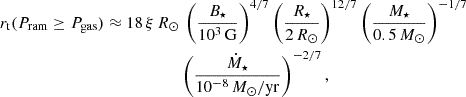 (2)
(2)
where B★ is the stellar magnetic field strength, R★ the stellar radius, M★ the stellar mass, and Ṁ★ the accretion rate on the star, and the correction factor (ξ) is 0.7 (Hartmann et al. 2016). For Pram < Pgas, the truncation radius follows from the condition
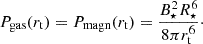 (3)
(3)
2.2. Stellar spin model
To calculate the stellar spin evolution, we included an external torque acting on the star,  , which equals the temporal derivative of the stellar AM, and the internal stellar evolution (e.g., Gallet et al. 2019). We assumed that the star rotates as a rigid body, J★ = Ω★I★, with the stellar moment of inertia, I★ = 0.2M★R★2 (e.g., Armitage & Clarke 1996; Matt et al. 2010)1. This results in a temporal derivative of the stellar angular velocity of
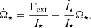 (4)
(4)
with
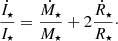 (5)
(5)
The external torque consists of the effects of the accretion process, Γacc, of the APSW, ΓAPSW, and of the ME, ΓME; Γext = Γacc + ΓAPSW + ΓME (see also Gallet et al. 2019; Gehrig et al. 2022). The accreted material carries AM that is added to the star and spins it up. An APSW removes AM from the star and causes a spin-down effect. MEs can spin up or spin down the star depending on the value of ωS. In the model of Gallet et al. (2019), MEs spin up the star for ωS ≤ 0.7.
Following Matt et al. (2010), the star contracts along the Hayashi track on its Kelvin-Helmholtz timescale2, resulting in a radius change according to
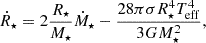 (6)
(6)
where Teff is the stellar effective temperature and σ the Stefan-Boltzmann constant. A detailed summary of the respective equations can be found in our previous work (Gehrig et al. 2022) and in Gallet et al. (2019).
2.3. Variable magnetic field
We studied the effects of a time-dependent magnetic field strength on two different timescales. First, the long-term effect of a decrease in the stellar dipole field strength due to the development of a radiative core was simulated (called the “long model”). According to Gregory et al. (2012), fully convective T Tauri stars host magnetic fields with a dominant dipole component of B★ ≳ 1 kG. Stars that have developed radiative cores, on the other hand, show more complex fields with dominant higher-order field components and weaker dipole fields of B★ ∼ 0.1 kG. Recent observations suggest that different dynamo mechanisms are responsible for generating the magnetic field in fully convective and partially convective stars (e.g., See et al. 2025), with notable differences particularly in the large-scale or dipole field strengths. It is assumed that the dipole component is the dominant component controlling the star–disk interaction (e.g., Finley & Matt 2018). The transition between these two states should occur within a few tenths of a megayear (e.g., Gregory et al. 2012; Villebrun et al. 2019). In our model, we started with a stellar dipole field of B★ = 1 kG at the beginning of the simulations. The initial stellar age, tinit, corresponds to the development of the radiative core and depends on the stellar mass (see Sect. 2.4 and Table 1). After a simulation time of τ0 = 104 years, B★ decreases and reaches 0.1 kG after τB = 0.5 Myr (see panel a of Fig. 1).
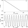 |
Fig. 1. Illustration of the time-dependent dipole field strength used in this work. Panel a: Long-term evolution due to the development of a radiative core. Panel b: Short-term variation due to stellar cycles. |
Initial model parameters used in this work.
Second, we included short-term variations due to stellar cycles (e.g., Armitage 1995, referred to as the “short model”). During a cycle period of τcyc, the stellar field strength varies according to
 (7)
(7)
where Bmean is the mean dipole field component and Bosc the oscillating field component. Again, we started with the variation of B★ after τ0 = 104 years. In fact, measurements of stellar dipole fields show a strong variability of B★ over several years. For example, the dipole field of V2129 Oph has increased from 280 G in 2005 to 970 G in 2009 (Johnstone et al. 2014). Based on the variation in photometric data of T Tauri stars ranging on timescales of 1.5 − 4 years (e.g., Lin et al. 2023), the cycle timescale can be estimated to be around ∼3 years (e.g., Gaidos et al. 2024). Furthermore, models of cool dwarfs (e.g., Bice & Toomre 2023) and solar-like stars (e.g., Strugarek et al. 2018) suggest plausible cycle timescales of ∼1 year and ∼30 years, respectively. Thus, we chose τcyc = 10 years (following Armitage 1995), Bmean = 1.0 kG, and Bosc = 0.9 kG. An illustration of B★(t) is given in Fig. 1b. Short-term variations of the stellar magnetic field of T Tauri stars are associated with a polarity reversal of the magnetic field (similar to the 11-year solar cycle; e.g., DeRosa et al. 2012; Finociety et al. 2023b; Gaidos et al. 2024). We note that the adopted form of the short-term magnetic cycle (Eq. 7) corresponds to an “effective” or absolute dipole field component acting on the disk. During a polarity reversal, the dipole field would decrease toward zero and change sign (as recently reported in Donati et al. 2026). For a dipole field close to zero, field components of higher order (quadrupole or octopole fields) start to affect the disk, resulting in an effective, nonzero component even at the polarity inversion (e.g., Finley & Matt 2018). In addition, we assumed that the alignment between the dipole field and the disk’s rotational axis is fixed. We discuss additional effects due to the changing alignment between the magnetic and rotational axes in Sect. 4.4. Further, the sinusoidal form of the cycle (following Armitage 1995) is an approximation. Observed magnetic field intensities in young stars show rather abrupt changes in the dipole component during possible polarity reversals (e.g., Finociety et al. 2023b). Although the exact form of the cycle remains unclear, the results of this work should not be significantly affected by a different cycle form. We chose the sinusoidal representation for its numerical stability.
2.4. List of parameters
Here, we provide an overview (see Table 1) of the parameters used in this work. We modeled three different stellar masses. To study the effects of a developing radiative core, we chose M★ = 1.0 and 0.7 M⊙. According to stellar evolution models, a solar mass star develops a radiative core shortly after 2 Myr and a 0.7 M⊙ star at around 5 Myr (e.g., Siess et al. 2000; Tognelli et al. 2011), which is the assumed stellar age at the beginning of the respective simulations, tinit. Magnetic cycles are also modeled for these stars, and, in addition, for a 0.3 M⊙ star with an initial age of 2 Myr. The initial stellar radii for the respective stars are based on isochrone models from Baraffe et al. (2015), and the initial accretion rates are chosen to be within the observed range reported in Betti et al. (2023). The viscosity parameters are taken from Cecil et al. (2024); αturb = 0.02 and αDZ = 0.0004. The initial rotation periods correspond to the respective ZTS (Γext ≈ 0) assuming an APSW efficiency of W = 1% and B★, init = 1.0 kG. The fastness parameter of the ZTS resulting from these input values is ωS ≈ 0.72, which matches the results of recent simulations (Zhu 2025) and population models (Gehrig et al. 2025). We initialized at ZTS rather than at spin equilibrium to isolate the effect of the variable magnetic field. We note that the star will spin up from stellar contraction in this configuration. Finally, we needed to choose the stellar X-ray luminosity, which is responsible for the photo-evaporative mass-loss. Recent developments in photo-evaporative models have shown lower mass-loss rates (by up to one order of magnitude) due to enhanced cooling (e.g., Sellek et al. 2024) compared to previous models (e.g., Ercolano et al. 2021). To get a mass-loss rate in our models that is comparable to the results presented in Sellek et al. (2024), we reduced the X-ray luminosities from Güdel et al. (2007) by a factor of 20.
3. Results
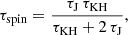
Before analyzing the evolution of the long and short models, we wanted to compare the relevant evolution timescales for the star–disk system (see Fig. 2). In the inner disk, the truncation radius adjusts on the order of days, equivalent to the dynamic timescale, τdyn, in ∼ days (e.g., Pittman et al. 2025), and the accretion rate evolves on the viscous timescale, τν, in ∼ 1000 years. The viscous timescale in the outer disk, τν, out ∼ 9 × 10⁵ years, is a measure for the long-term evolution of the disk accretion rate and the disk lifetime. The stellar spin evolves on a timescale  that combines the effect of the external torques and of stellar contraction. Neglecting the slow change of the stellar mass, Eqs. (4)–(6) yield
 (8)
(8)
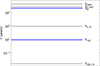 |
Fig. 2. Evolution timescales of the star–disk system relevant for this work. The timescales on which the magnetic field is assumed to change are marked in blue. |
where  is the timescale associated with the external (accretion + spin-down) torques and τKH = R★/|Ṙ★| is the Kelvin-Helmholtz timescale set by the second term on the right-hand side of Eq. (6). The external-torque timescale τJ is not constant: it can reach ∼(1 − 2)×106 yr in the spin-down regime at large fastness parameters (e.g., Ireland et al. 2022), but becomes considerably shorter in an accretion-dominated spin-up regime. For our initial conditions, the system starts in a ZTS (τJ → ∞), and τspin is set by contraction, τspin ≈ τKH/2 of approximately a few megayears. Once the simulation starts and the value of B★ changes, the star moves out of the ZTS, and τJ becomes variable. During our simulations, τspin stays at values of ≳τν, out. Depending on the relation between these timescales and τB = 5 × 10⁵ years and τcyc = 10 years, we expect different reactions of the disk on the variation of B★. Since τB ≫ τν, in ≫ τdyn, in, we expect that the inner disk quickly adjusts to magnetic variations due to a growing radiative core. The long-term evolution of the disk and the stellar rotation period, on the other hand, should only slowly adjust to the new magnetic field strength as τB < τν, out < τspin. In the case of magnetic cycles, the viscous timescales in the disk and the stellar spin evolution timescale are slow to react to the short-term changes in B★. The position of the truncation radius, however, should adjust to the variations quickly. Thus, we can expect a nontrivial reaction in the inner disk due to the short magnetic cycles. Overall, the stellar spin evolution (and the position of the corotation radius) is slow to react to changes in the magnetic field, and the truncation radius adjusts quickly. Thus, we expect the stellar spin state, defined by the fastness parameter ωs, to be directly affected by a variable B★.
We started our simulations with a star in the ZTS with a fastness parameter of ωS ≈ 0.72. After τ0 = 104 years, the temporal variation of B★ begins. In Fig. 3, the results for the long model are shown for stellar masses of 1.0 and 0.7 M⊙. For comparison, we include simulations in which the magnetic field remains constant. With a decrease in B★ after τ0 = 104 years, the truncation radius decreases according to Eq. (2) almost instantly on a timescale τdyn, in (panel b). The stellar rotation period and the corotation radius remain approximately constant as the stellar spin evolves on a larger timescale τspin (see Fig. 2). Consequently, the fastness parameter decreases from its initial value of 0.72 toward ≈0.17 (or by a factor of ≈4). As long as the accretion rate remains above Ṁ★ ≳ 10−9 M⊙ yr−1, the stellar spin slowly adjusts to the new condition, the star spins up, and ωs increases over the next few million years. As the accretion rate decreases due to viscous evolution and PE, the truncation radius increases, ultimately resulting in a value of ωS ≈ 1 as the accretion rate drops toward zero. During their T Tauri lifetime, stars at different masses (M★ ≳ 0.7 M⊙) start to develop a radiative core at different ages, and for all these different stellar masses, observations show a significant scatter in accretion rates. As a result, numerous combinations of stellar masses, ages, and accretion rates yield different rotation periods in their respective ZTS. For both stellar masses, which are shown here at different ages, the effect of a decreasing dipole field strength due to the development of a radiative core is similar.
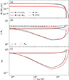 |
Fig. 3. Evolution of the long model compared to simulations with a constant magnetic field strength. The initial stellar ages of the 1.0 and 0.7 M⊙ models are tinit = 2.0 and 5.0 Myr (see Table 1), respectively. Panel a: Accretion rate. Panel b: Truncation radius, rt, and the corotation radius, Rco, in units of the stellar radius. Panel c: Fastness parameter, ωS. |
In the case of stellar magnetic cycles, the corresponding timescale τcyc = 10 years is significantly smaller than the stellar or disk evolution timescales. Thus, we assumed that the stellar radius remains constant over several τcyc. In contrast to the development of a radiative core, stellar magnetic cycles can also affect smaller stars that remain fully convective during their disk phase. The evolution of the short model for three different stellar masses, ages, and accretion rates is shown in Fig. 4. With an increasing magnetic field strength, the truncation radius is pushed away from the star (see Eq. (2)). The disk material cannot adjust to the change in the truncation radius as the viscous timescale in the inner disk is significantly larger compared to the cycles timescale (τν, in/τcyc ≳ 100). As a consequence, more disk material is located inside rt and is accreted on the star, increasing the accretion rate (panel a). Similarly, as B★ decreases, the disk material cannot follow the decreasing truncation radius, and the accretion rate also decreases. We note that for all our simulations the condition rt < Rco or ωS < 1 is fulfilled. Should the increase in magnetic field strength push the truncation radius beyond the corotation radius, disk material would be propelled away from the star and the accretion rate would significantly drop (e.g., Armitage 1995; Romanova et al. 2004a). The slow back-reaction in the accretion rate (τν, in > τcyc) weakens the effect of the magnetic cycles on the ZTS (the change in the accretion rate has an opposite effect on rt compared to the variable magnetic field, panel c and Eq. (2)). During one cycle, ωs varies between 0.87 and 0.50 (or by a factor of 1.74). Although the absolute values vary, the overall behavior of the accretion rate and ωS is comparable for the different stellar masses, ages, and accretion rates.
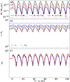 |
Fig. 4. Evolution of the short model. The panels are the same as in Fig. 3. The time reference is the beginning of the magnetic cycles at a simulation time of τ0 = 104 years. |
4. Discussion
4.1. Comparison with observations
Recently, the truncation radius of T Tauri stars has been derived from observational data in combination with the stellar rotation period and the corotation radius for a few dozen stars (Thanathibodee et al. 2023; Pittman et al. 2025). In both cases, a significant number of stars show values ωS smaller than expected from stellar spin models (e.g., Ireland et al. 2022; Serna et al. 2024; Zhu 2025). Based on the results presented in Pittman et al. (2025), we wanted to compare the ωS values of fully convective stars and stars that have started to develop a radiative core. For this comparison, we selected stars with stellar masses of M★ ≥ 0.7 M⊙ (see Table 2). For these stellar masses, the radiative core is expected to develop within the first 5 Myr of their lifetimes. For each star, we compared the stellar age taken from the literature with the end of the fully convective phase τconv based on the stellar evolution models of Tognelli et al. (2011, see also Gregory et al. 2012).
![Mathematical equation: $$ \begin{aligned} \tau _{\rm conv}\,\mathrm{[Myr]} \approx \left(\frac{1.448}{M_\star /M_\odot }\right)^{2.101}. \end{aligned} $$](/articles/aa/full_html/2026/06/aa58330-25/aa58330-25-eq12.gif) (9)
(9)
Mean stellar parameters from Pittman et al. (2025), including stellar ages taken from the literature.
We note that a minimum value of ωS should be reached at around τB = 0.5 Myr after the radiative core starts to develop (see Fig. 3). For a 1.0 M⊙ star, this results in a stellar age of τconv + τB ≈ 2.6 Myr and for a 0.7 M⊙ star, in an age of τconv + τB ≈ 5.1 Myr according to Eq. (9). We distinguish between stars with ages older (“old” stars) and younger (“young” stars) than τconv + τB and compare the values of ωS in Fig. 5. For young stars, the mean fastness parameter is ωS = 0.55 ± 0.40 and for old stars, ωS = 0.24 ± 0.16. The values for young stars are consistent with the ZTS for a spin model including an APSW (see Gehrig et al. 2025). The values for old stars match the simulation results shown in Fig. 3b.
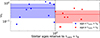 |
Fig. 5. Comparison of the values of ωS of the young (ages < τconv + τB) and old (ages ≥ τconv + τB) stars listed in Table 2. The stellar ages are plotted relative to τconv + τB (marked by the vertical dashed line). The horizontal lines show the respective mean values, and the colored areas mark the respective standard deviations. |
While this initial comparison suggests an age trend in ωS, we note that some caution remains warranted. First of all, the small number of available observations and the resulting uncertainties require more measurements to draw a clear conclusion. The two stars with the largest values of ωS, MY Lup and CV Cha, are in the regime τconv < age < τconv + τB. According to Fig. 3, some initial effects of the decreasing dipole field component on ωS should already be noticeable. Although this dataset is not fully consistent with the results presented in this work, the observational uncertainties should be taken into account. The inner disk radius and, in turn, ωS are subjected to short-term variability, for example, due to variability in the accretion rate (e.g., Zsidi et al. 2022; Robinson et al. 2022). In the case of MY Lup, the value of ωS varies from 0.55 to 1.42 during the observations (Pittman et al. 2025). Further, mass and age estimates can vary significantly depending on the observation method itself (e.g., Flores et al. 2022). For example, the age of CV Cha is reported to be 1.3−1.5 Myr (from which the mean value was used in Table 2; Ginski et al. 2024) and 3.0 − 4.5 Myr (Gregory et al. 2012). Another potential source of uncertainty in stellar age estimates is the disk itself. A large inclination (as in the case of MY Lup) and flaring can extinct the host star, leading to an overestimation of the stellar age (e.g., Andrews et al. 2018). As a result, the age of MY Lup has been corrected from 16.6 Myr, as reported in Frasca et al. (2017), to 2 Myr (Long et al. 2022). In addition, the effects of binaries and magnetic stellar evolution models (e.g., Feiden 2016) are not included in this preliminary comparison.
We further note that the value of ωS should increase again due to decreasing accretion rates toward the end of the disk’s lifetime (see Fig. 3). For all but two stars from the sample of Pittman et al. (2025), the accretion rate shows values of Ṁ★ > 10−9 M⊙ yr−1 even at older ages, and small values of ωS are expected after the radiative core has formed, matching our results. The accretion rates provided by Thanathibodee et al. (2023), on the other hand, range at Ṁ★ ∼ 10−10 M⊙ yr−1 and they find values of ωS ≲ 0.45 for most stars in their study, contradicting our results. As discussed in Thanathibodee et al. (2023), the mechanisms that shape the final stages of disk accretion in T Tauri stars have to be studied in future work. However, analyzing the stellar spin state (e.g., by means of the fastness parameter) at different stellar evolutionary stages (e.g., age < τconv, age ≈ τconv, and age > τconv) can advance our understanding of the star–disk interaction. One mission that could provide the fastness parameter for many stars is the Early eVolution Explorer (EVE) satellite (MacGregor et al. 2025). With a combined derivation of the truncation radius, the accretion rate, and the stellar rotation period, EVE can increase the available data by a factor of ≳15.
Comparing our results on magnetic cycles with observational data proves to be no less challenging. While variation in the dipole field strengths on the timescales of years have been known for a few stars (e.g., Johnstone et al. 2014; Finociety et al. 2023a; Gaidos et al. 2024), the first magnetic polarity reversal of a T Tauri star has been reported recently (for the star DO Tau, see Donati et al. 2026). A suitable comparison with our results requires simultaneous measurements of the dipole field strength, the truncation radius (that can be calculated with the accretion rate and the dipole field strength Bessolaz et al. 2008; Hartmann et al. 2016), and the stellar rotation period (setting the corotation radius). The SpectroPolarimetre InfraRouge (SPIRou) Legacy Survey does provide these measurements (e.g., Donati et al. 2020, 2024, 2026). In the course of the survey, young, accreting stars show variations of the dipole field strengths on timescales of several years. The dipole strength of V1298 Tau decreases from 245 G to 85 G (a factor of almost 3) during one year (Finociety et al. 2023a) and during the polarity reversal of DO Tau, the dipole field evolves from −190 G to 320 G (Donati et al. 2026). The absolute change of the dipole field in these stars is relatively small (∼100 G) compared to the present study and effects on the accretion rate are not clearly measurable. Larger dipole variations are reported for V2129 Oph from 280 G in 2005 to 970 G in 2009 (Johnstone et al. 2014). Unfortunately, the accretion rates have not been measured simultaneously and the effect of the different dipole field strengths on the accretion rate, the truncation radius, and the stellar spin state cannot be estimated. Future results by surveys like SPIRou will provide valuable data for constraining stellar magnetic cycles and their effects on the stellar spin evolution.
4.2. Other factors affecting the stellar spin state
During the evolution of a T Tauri star, other factors can affect the stellar spin state through the truncation radius or the corotation radius. In terms of the truncation radius, the most volatile contributing factors are the magnetic field strength and the accretion rate (see Eq. 2). The accretion rate can be variable on timescales of days to years (see the review by Fischer et al. 2023). Observations show a routine variability of < 1 − 2 mag over days to years (matching the dynamic and viscous timescale of the inner disk; e.g., Cody et al. 2017). In addition, outburst events can increase the accretion rate by up to 6 mag and can last for years to decades (e.g., Fu Ori outbursts; Kóspál et al. 2011). While we have observed a back-reaction of the accretion rate on the stellar magnetic cycles, there are other reasons for a variable Ṁ★ that are independent of B★ (e.g., Fischer et al. 2023). According to Eq. (2), a one-order-of-magnitude increase in the accretion rate will push the truncation radius inward by a factor of 0.52, corresponding to a decrease in ωs by 63%. Together with the effect of a stellar magnetic cycle, the value of ωs can be decreased even further. The potential combination of these effects could lead to a significant deviation from the ZTS.
Another factor that can affect the stellar spin state of observed stars is the assumed spin model itself. The ZTS value of ωs varies with different spin models, as the torque contributions acting on the star are subject to change with theoretical and observational advances (e.g., Ireland et al. 2021, 2022; Takasao et al. 2025; Zhu 2025). In their 3D model, for example, Takasao et al. (2025) found that MEs might play only a minor role in the stellar spin evolution, whereas CDWs can potentially remove significant amounts of disk and stellar AM (comparable to a strong APSW). An additional torque contribution that removes stellar AM, similar to an APSW, can result in smaller ωS values in the ZTS (Gehrig et al. 2025). Unfortunately, these recent models are restricted to a limited parameter space due to high computational costs (e.g., Takasao et al. 2022; Zhu 2025), and generalizing the results might not be straightforward.
This apparent incompleteness of the stellar spin model can be illustrated by the evolution of the stellar rotation period. In Fig. 6 we show the rotation period of the long model for a stellar mass of 1.0 M⊙ (see also Fig. 3). For comparison, the stellar rotation period of a contracting star according to Eq. (6) without any external torque contributions is highlighted. With a decreasing stellar magnetic field strength and low values of ωS, a spin-up torque is exerted onto the star in addition to its contraction, leading to fast rotation periods. This spin-up contradicts the observed constancy of rotational distributions (e.g., Smith et al. 2023), which indicates that certain spin-down contributions are not yet completely covered by the stellar spin model, as stated above, for example, the effects of winds in the innermost disk region.
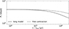 |
Fig. 6. Evolution of the stellar rotation period of the long model for a stellar mass of 1.0 M⊙. The rotation period of a contracting star according to Eq. (6) without any external torque contributions is shown for comparison. |
4.3. Dependence on timescales
We have shown the effects of a variable B★ based on two different scenarios acting on two different timescales. These timescales, however, might vary according to different stellar masses or ages. First, we show how the long model reacts if we change τB to 105 years and 2 × 10⁶ years. The stellar spin reacts to a changing magnetic field strength on timescales of τspin ≳ 2 − 3 Myr (see Fig. 3). If the timescale on which the magnetic field changes is significantly smaller, τB ≪ τspin, the stellar spin cannot adjust to the new parameters and the relative effect on ωS is large (blue lines in Fig. 7). For increasing values of τB ∼ τspin, the stellar spin can be adjusted to the changing parameter, and the relative effect on ωS is weaker (red lines in Fig. 7). If τB were much larger than τspin, we would not expect a significant shift away from the ZTS. In addition to the adjustment of the stellar spin to the new magnetic field strength, the decrease in the accretion rate due to the disk evolution and PE can limit the effect on ωs in the case of large values of τB.
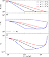 |
Fig. 7. Effect of different values of τB on the long model. The stellar mass is 1.0 M⊙. Panel a: Dipole field strength, B★. Panels b and c: Same as in Fig. 3. |
For variations in magnetic field strength on shorter timescales, we show how different values of τcyc affect the evolution of ωs (see Fig. 8). As shown in Fig. 4, the disk material is slow to adjust to variations shorter than the viscous timescale in the inner disk (τcyc < τν, in ≈ 1000 years, black lines). As a result, the accretion rate is affected by the magnetic cycle (the variable accretion rate has an opposite effect on rt compared to the variable magnetic field), and the effect on ωS is weakened. For increasing values of τcyc = τν, in, the disk material can adjust to the magnetic field variation, and enough disk material can be redistributed within the inner disk. As a result, the effect of a variable magnetic field on the accretion rate becomes smaller for increasing values of τcyc, and the accretion rate remains closer to its initial value. Thus, the ωS is shifted further away from its ZTS (blue lines). For even larger values τν, in < τcyc = 104 years, ωs is pushed toward values of ∼0.2 (red lines)3. While ωs is shifted significantly toward smaller values as a result of a decreasing field strength during a magnetic cycle, the shift toward larger values is weaker. When the truncation radius is pushed outward by an increasing magnetic field, the disk pressure increases close to the corotation radius (e.g., Steiner et al. 2021; Ireland et al. 2022), preventing a further outward shift. Summarizing, the effect of short-term magnetic variations on ωS depends on the relation between τcyc and the viscous timescale of the inner disk τν, in. A shift of the disk’s inner radius toward the star will also increase the temperature structure of the innermost disk regions. If the temperature increase is sufficient to ionize enough disk material, magneto-rotational instabilities can be triggered, causing further variability. These effects, however, are beyond the scope of this work and might be the subject of future studies.
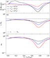 |
Fig. 8. Effect of different values of τcyc on the short model. The stellar mass is 1.0 M⊙. The time axis is normalized to one cycle, starting at τ0. The panels are the same as in Fig. 3. |
As mentioned in Sect. 2, the current model does not include the effects of magnetohydrodynamic-driven disk winds. There is growing theoretical and observational evidence that disk winds are essential for the evolution of PPDs (e.g., Zhu & Stone 2018; Jacquemin-Ide et al. 2021; Pascucci et al. 2023; van Dishoeck et al. 2025; Zhu 2025; Feeney-Johansson et al. 2026). Within the context of the present work, we want to discuss the effect of such disk winds on our results. The effect of a variation in the stellar magnetic field on the spin state depends on how fast the disk can react to changes in field strength. In a disk evolution scenario dominated by magnetohydrodynamic winds, the accretion timescale, τacc, is expected to be shorter compared to the viscous timescale. Models yield estimates of around τacc ∼ 100 × τdyn (e.g., Jacquemin-Ide et al. 2021). In the outer disk regions, this is comparable to the viscous timescale (see also Tabone et al. 2021), and our results should also apply to the wind-driven scenario. In the inner disk, on the other hand, the accretion timescale is significantly shorter than the viscous timescale, τacc ≲ τcyc ≪ τν, in (see also Fig. 2). As a result, material in the inner disk would react more quickly, and the stellar spin state should become more sensitive to variations in the stellar magnetic field strength (this would be comparable to larger values of τcyc in Fig. 8). The precise effects of disk winds on the stellar spin state will be the subject of future studies of this model, extended with magnetohydrodynamic-driven winds (with the fundamentals already included in Steiner et al. 2025).
4.4. Further implications for the inner disk
In this work, we did not include the large-scale disk magnetic field (for recent developments we refer to Steiner et al. 2025) or the effects resulting from the reversal of the magnetic field’s polarity (see Sect. 2.3). However, the stellar magnetic field can dominate the large-scale magnetic field topology in the inner disk region (see Steiner et al. 2025). Recent 3D simulations of the star-disk connection have shown that only a very limited region of the disk is directly connected to the star (r ≲ Rco; e.g., Takasao et al. 2022; Zhu 2025). Stellar field lines threading the disk at larger radii open up and are not able to transfer AM between the star and the disk. However, a changing polarity of the stellar magnetic field has implications on the resulting magnetic field strength and wind launching mechanisms (e.g., Ferreira et al. 2006) in the very inner disk:
-
(i)
In the anti-aligned case, magnetic flux, transported inward by magnetic advection, builds up close to the inner disk region, where the stellar magnetic field is strong enough to support closed field lines. This leads to an increased magnetic field strength in the vicinity of the magnetic truncation radius. In this configuration, an out-bursting, reoccurring outflow (for example, MEs) can transport AM between the star and the disk (e.g., Romanova et al. 2009; Zanni & Ferreira 2013).
-
(ii)
In the aligned case, the magnetic flux can merge/reconnect with the stellar magnetic field. At the point, where the stellar field “cancels out” the disk field (the so-called X-point), open field lines can connect to the closed stellar field lines and remove AM (e.g., Ferreira et al. 2000).
An oscillating polarity therefore likely leads to a time-dependent change in magnetic field strength and field topology close to the inner disk rim. This has an impact on the possibility and strength outflows originating from the innermost disk region (e.g., Lesur et al. 2023). Thus, periodically changing stellar fields could be a possible source of time-dependent disk winds. Recent observations of disk outflows and jets show “knotty” jets, which could be caused by a change in the magnetic field polarity (e.g., Vorobyov et al. 2018; Bajaj et al. 2025). To study the effects of changing magnetic field polarity on the inner disk and winds, future models should combine: (i) the innermost disk region including the magnetic star-disk connection, (ii) a description of the large-scale magnetic field, and (iii) a wind model, describing the launch of magneto-centrifugal and magneto-thermal winds.
5. Summary
In this work we show that the temporal variation of the stellar dipole field strength (B★) can have a distinct effect on the stellar spin state, described by the fastness parameter (ωs). Observations have shown significantly lower values of ωs than expected from stellar spin models. Two potential scenarios of a variable magnetic field have been studied. First, the decrease in B★ due to the development of a radiative core on a timescale of τB = 0.1 − 2.0 Myr (long model). Second, the variability of B★ due to stellar magnetic cycles with τcyc = 101 − 104 years (short model). The strength of these variations depends on the relation between the timescale of the changing magnetic field (τB or τcyc), the spin-up timescale (τspin), and the viscous timescale of the accretion disk (τν).
In the case of τB ≪ τspin ∼ 2 − 3 Myr, the stellar spin is slow to adjust to the changing parameters, and ωS is shifted out of its ZTS. If the variations occur on long timescales τB ∼ τspin, the stellar spin can adjust to the change and remain closer to its ZTS. On shorter timescales, the effect of magnetic cycles on ωS is weaker if they occur on shorter timescales than the viscous timescale of the inner disk τcyc ≪ τν, in ∼ 103 years. The inner disk material is slow to adjust to the changing parameters, resulting in a back-reaction in the accretion rate. For τcyc ≫ τν, in, this back-reaction is less pronounced and the effect on ωS increases. Our results can explain at least part of the observed low values ωs. Another possibility that could explain the differences between expected and measured ωS values is outflows and winds from the inner disk region. These winds can transport significant amounts of AM and affect the stellar spin state. In the next iteration of our star-disk model, we focus on these (time-dependent) disk winds in different configurations. We encourage further theoretical and observational work that connects accretion, stellar rotation, and magnetic properties in T Tauri stars.
Acknowledgments
The authors thank the anonymous referees for constructive feedback and insightful comments that improved the clarity of this work. Furthermore, we thank Eric Gaidos for his valuable comments during the course of the work. All figures were created using the Python packages Matplotlib (Hunter 2007) and Numpy (Harris et al. 2020).
References
- Agapitou, V., & Papaloizou, J. C. B. 2000, MNRAS, 317, 273 [CrossRef] [Google Scholar]
- Andrews, S. M., Terrell, M., Tripathi, A., et al. 2018, ApJ, 865, 157 [Google Scholar]
- Armitage, P. J. 1995, MNRAS, 274, 1242 [NASA ADS] [Google Scholar]
- Armitage, P. J., & Clarke, C. J. 1996, MNRAS, 280, 458 [NASA ADS] [Google Scholar]
- Armitage, P. J., Livio, M., & Pringle, J. E. 2001, MNRAS, 324, 705 [NASA ADS] [CrossRef] [Google Scholar]
- Bajaj, N. S., Pascucci, I., Beck, T. L., et al. 2025, AJ, 169, 296 [Google Scholar]
- Baraffe, I., Homeier, D., Allard, F., & Chabrier, G. 2015, A&A, 577, A42 [NASA ADS] [CrossRef] [EDP Sciences] [Google Scholar]
- Bessolaz, N., Zanni, C., Ferreira, J., Keppens, R., & Bouvier, J. 2008, A&A, 478, 155 [NASA ADS] [CrossRef] [EDP Sciences] [Google Scholar]
- Betti, S. K., Follette, K. B., Ward-Duong, K., et al. 2023, AJ, 166, 262 [Google Scholar]
- Biazzo, K., Frasca, A., Alcalá, J. M., et al. 2017, A&A, 605, A66 [NASA ADS] [CrossRef] [EDP Sciences] [Google Scholar]
- Bice, C. P., & Toomre, J. 2023, ApJ, 947, 36 [NASA ADS] [CrossRef] [Google Scholar]
- Cecil, M., Gehrig, L., & Steiner, D. 2024, A&A, 687, A136 [NASA ADS] [CrossRef] [EDP Sciences] [Google Scholar]
- Cody, A. M., & Hillenbrand, L. A. 2010, ApJS, 191, 389 [NASA ADS] [CrossRef] [Google Scholar]
- Cody, A. M., Hillenbrand, L. A., David, T. J., et al. 2017, ApJ, 836, 41 [Google Scholar]
- DeRosa, M. L., Brun, A. S., & Hoeksema, J. T. 2012, ApJ, 757, 96 [NASA ADS] [CrossRef] [Google Scholar]
- Donati, J.-F., Skelly, M. B., Bouvier, J., et al. 2010, MNRAS, 409, 1347 [NASA ADS] [CrossRef] [Google Scholar]
- Donati, J.-F., Kouach, D., Moutou, C., et al. 2020, MNRAS, 498, 5684 [NASA ADS] [CrossRef] [Google Scholar]
- Donati, J. F., Finociety, B., Cristofari, P. I., et al. 2024, MNRAS, 530, 264 [NASA ADS] [CrossRef] [Google Scholar]
- Donati, J.-F., Cristofari, P. I., Carmona, A., et al. 2026, A&A, 708, A230 [NASA ADS] [CrossRef] [EDP Sciences] [Google Scholar]
- Dorfi, E., & Drury, L. 1987, J. Comput. Phys., 69, 175 [NASA ADS] [CrossRef] [Google Scholar]
- Ercolano, B., Picogna, G., Monsch, K., Drake, J. J., & Preibisch, T. 2021, MNRAS, 508, 1675 [NASA ADS] [CrossRef] [Google Scholar]
- Feeney-Johansson, A., Aikawa, Y., Takakuwa, S., et al. 2026, AJ, 171, 172 [Google Scholar]
- Feiden, G. A. 2016, A&A, 593, A99 [NASA ADS] [CrossRef] [EDP Sciences] [Google Scholar]
- Ferreira, J., Pelletier, G., & Appl, S. 2000, MNRAS, 312, 387 [NASA ADS] [CrossRef] [Google Scholar]
- Ferreira, J., Dougados, C., & Cabrit, S. 2006, A&A, 453, 785 [NASA ADS] [CrossRef] [EDP Sciences] [Google Scholar]
- Finley, A. J., & Matt, S. P. 2018, ApJ, 854, 78 [Google Scholar]
- Finociety, B., Donati, J.-F., Cristofari, P. I., et al. 2023a, MNRAS, 526, 4627 [NASA ADS] [CrossRef] [Google Scholar]
- Finociety, B., Donati, J. F., Grankin, K., et al. 2023b, MNRAS, 520, 3049 [NASA ADS] [CrossRef] [Google Scholar]
- Fischer, W. J., Hillenbrand, L. A., Herczeg, G. J., et al. 2023, ASP Conf. Ser., 534, 355 [NASA ADS] [Google Scholar]
- Flores, C., Connelley, M. S., Reipurth, B., & Duchêne, G. 2022, ApJ, 925, 21 [NASA ADS] [CrossRef] [Google Scholar]
- Frasca, A., Biazzo, K., Alcalá, J. M., et al. 2017, A&A, 602, A33 [NASA ADS] [CrossRef] [EDP Sciences] [Google Scholar]
- Gaidos, E., Thanathibodee, T., Hoffman, A., et al. 2024, ApJ, 966, 167 [NASA ADS] [CrossRef] [Google Scholar]
- Gallet, F., & Bouvier, J. 2013, A&A, 556, A36 [NASA ADS] [CrossRef] [EDP Sciences] [Google Scholar]
- Gallet, F., Zanni, C., & Amard, L. 2019, A&A, 632, A6 [NASA ADS] [CrossRef] [EDP Sciences] [Google Scholar]
- Gammie, C. F. 1996, ApJ, 457, 355 [Google Scholar]
- Gehrig, L., Steiner, D., Vorobyov, E. I., & Güdel, M. 2022, A&A, 667, A46 [NASA ADS] [CrossRef] [EDP Sciences] [Google Scholar]
- Gehrig, L., Gaidos, E., Venuti, L., Cody, A. M., & Turner, N. J. 2025, A&A, 696, L18 [NASA ADS] [CrossRef] [EDP Sciences] [Google Scholar]
- Ghosh, P. 2007, Rotation and Accretion Powered Pulsars (World Scientific), 10 [Google Scholar]
- Ghosh, P., & Lamb, F. K. 1979, ApJ, 234, 296 [Google Scholar]
- Ginski, C., Garufi, A., Benisty, M., et al. 2024, A&A, 685, A52 [NASA ADS] [CrossRef] [EDP Sciences] [Google Scholar]
- GRAVITY Collaboration (Bouarour, Y. I., et al.) 2020, A&A, 642, A162 [NASA ADS] [CrossRef] [EDP Sciences] [Google Scholar]
- Gregory, S. G., Donati, J. F., Morin, J., et al. 2012, ApJ, 755, 97 [Google Scholar]
- Güdel, M., Briggs, K. R., Arzner, K., et al. 2007, A&A, 468, 353 [Google Scholar]
- Harris, C. R., Millman, K. J., van der Walt, S. J., et al. 2020, Nature, 585, 357 [NASA ADS] [CrossRef] [Google Scholar]
- Hartmann, L., Herczeg, G., & Calvet, N. 2016, ARA&A, 54, 135 [Google Scholar]
- Herbst, W., Bailer-Jones, C. A. L., Mundt, R., Meisenheimer, K., & Wackermann, R. 2002, A&A, 396, 513 [EDP Sciences] [Google Scholar]
- Herbst, W., Eislöffel, J., Mundt, R., & Scholz, A. 2007, in Protostars and Planets V, eds. B. Reipurth, D. Jewitt, & K. Keil, 297 [Google Scholar]
- Hunter, J. D. 2007, Comput. Sci. Eng., 9, 90 [NASA ADS] [CrossRef] [Google Scholar]
- Ireland, L. G., Zanni, C., Matt, S. P., & Pantolmos, G. 2021, ApJ, 906, 4 [Google Scholar]
- Ireland, L. G., Matt, S. P., & Zanni, C. 2022, ApJ, 929, 65 [NASA ADS] [CrossRef] [Google Scholar]
- Jacquemin-Ide, J., Lesur, G., & Ferreira, J. 2021, A&A, 647, A192 [EDP Sciences] [Google Scholar]
- Johnstone, C. P., Jardine, M., Gregory, S. G., Donati, J. F., & Hussain, G. 2014, MNRAS, 437, 3202 [Google Scholar]
- Koenigl, A. 1991, ApJ, 370, L39 [Google Scholar]
- Koldoba, A. V., Lovelace, R. V. E., Ustyugova, G. V., & Romanova, M. M. 2002, AJ, 123, 2019 [NASA ADS] [CrossRef] [Google Scholar]
- Kóspál, Á., Ábrahám, P., Acosta-Pulido, J. A., et al. 2011, A&A, 527, A133 [NASA ADS] [CrossRef] [EDP Sciences] [Google Scholar]
- Lavail, A., Kochukhov, O., & Hussain, G. A. J. 2019, A&A, 630, A99 [NASA ADS] [CrossRef] [EDP Sciences] [Google Scholar]
- Lehtinen, J. J., Käpylä, M. J., Hackman, T., et al. 2022, A&A, 660, A141 [NASA ADS] [CrossRef] [EDP Sciences] [Google Scholar]
- Lesur, G., Flock, M., Ercolano, B., et al. 2023, ASP Conf. Ser., 534, 465 [NASA ADS] [Google Scholar]
- Lii, P. S., Romanova, M. M., Ustyugova, G. V., Koldoba, A. V., & Lovelace, R. V. E. 2014, MNRAS, 441, 86 [Google Scholar]
- Lin, C.-L., Ip, W.-H., Hsiao, Y., et al. 2023, AJ, 166, 82 [NASA ADS] [CrossRef] [Google Scholar]
- Long, F., Andrews, S. M., Rosotti, G., et al. 2022, ApJ, 931, 6 [NASA ADS] [CrossRef] [Google Scholar]
- MacGregor, M., Cody, A. M., Turner, N., et al. 2025, Am. Astron. Soc. Meet. Abstr., 245, 234.09 [Google Scholar]
- Matt, S., & Pudritz, R. E. 2005a, ApJ, 632, L135 [Google Scholar]
- Matt, S., & Pudritz, R. E. 2005b, MNRAS, 356, 167 [NASA ADS] [CrossRef] [Google Scholar]
- Matt, S. P., Pinzón, G., de la Reza, R., & Greene, T. P. 2010, ApJ, 714, 989 [NASA ADS] [CrossRef] [Google Scholar]
- Matt, S. P., MacGregor, K. B., Pinsonneault, M. H., & Greene, T. P. 2012, ApJ, 754, L26 [Google Scholar]
- Maucó, K., Hernández, J., Calvet, N., et al. 2016, ApJ, 829, 38 [CrossRef] [Google Scholar]
- Ménard, F., Cuello, N., Ginski, C., et al. 2020, A&A, 639, L1 [EDP Sciences] [Google Scholar]
- Pantolmos, G., Zanni, C., & Bouvier, J. 2020, A&A, 643, A129 [NASA ADS] [CrossRef] [EDP Sciences] [Google Scholar]
- Pascucci, I., Cabrit, S., Edwards, S., et al. 2023, ASP Conf. Ser., 534, 567 [NASA ADS] [Google Scholar]
- Pittman, C. V., Espaillat, C. C., Robinson, C. E., et al. 2022, AJ, 164, 201 [NASA ADS] [CrossRef] [Google Scholar]
- Pittman, C. V., Espaillat, C. C., Zhu, Z., et al. 2025, ApJ, 993, 181 [Google Scholar]
- Pringle, J. E. 1981, ARA&A, 19, 137 [NASA ADS] [CrossRef] [Google Scholar]
- Ragossnig, F., Dorfi, E. A., Ratschiner, B., et al. 2020, Comput. Phys. Commun., 256, 107437 [NASA ADS] [CrossRef] [Google Scholar]
- Rebull, L. M. 2001, AJ, 121, 1676 [NASA ADS] [CrossRef] [Google Scholar]
- Rebull, L. M., Wolff, S. C., Strom, S. E., & Makidon, R. B. 2002, AJ, 124, 546 [Google Scholar]
- Rebull, L. M., Stauffer, J. R., Megeath, S. T., Hora, J. L., & Hartmann, L. 2006, ApJ, 646, 297 [NASA ADS] [CrossRef] [Google Scholar]
- Rebull, L. M., Stauffer, J. R., Cody, A. M., et al. 2020, AJ, 159, 273 [Google Scholar]
- Robinson, C. E., Espaillat, C. C., & Rodriguez, J. E. 2022, ApJ, 935, 54 [NASA ADS] [CrossRef] [Google Scholar]
- Roccatagliata, V., Henning, T., Wolf, S., et al. 2009, A&A, 497, 409 [NASA ADS] [CrossRef] [EDP Sciences] [Google Scholar]
- Romanova, M. M., Ustyugova, G. V., Koldoba, A. V., & Lovelace, R. V. E. 2002, ApJ, 578, 420 [Google Scholar]
- Romanova, M. M., Ustyugova, G. V., Koldoba, A. V., & Lovelace, R. V. E. 2004a, ApJ, 616, L151 [CrossRef] [Google Scholar]
- Romanova, M. M., Ustyugova, G. V., Koldoba, A. V., & Lovelace, R. V. E. 2004b, ApJ, 610, 920 [Google Scholar]
- Romanova, M. M., Ustyugova, G. V., Koldoba, A. V., & Lovelace, R. V. E. 2009, MNRAS, 399, 1802 [Google Scholar]
- Romanova, M., Blinova, A., Ustyugova, G., Koldoba, A., & Lovelace, R. 2018, New Astron., 62, 94 [Google Scholar]
- Rugel, M., Fedele, D., & Herczeg, G. 2018, A&A, 609, A70 [NASA ADS] [CrossRef] [EDP Sciences] [Google Scholar]
- See, V., Amard, L., Bellotti, S., et al. 2025, MNRAS, 542, 1318 [Google Scholar]
- Sellek, A. D., Grassi, T., Picogna, G., et al. 2024, A&A, 690, A296 [NASA ADS] [CrossRef] [EDP Sciences] [Google Scholar]
- Serna, J., Hernandez, J., Kounkel, M., et al. 2021, ApJ, 923, 177 [NASA ADS] [CrossRef] [Google Scholar]
- Serna, J., Pinzón, G., Hernández, J., et al. 2024, ApJ, 968, 68 [NASA ADS] [CrossRef] [Google Scholar]
- Shakura, N., & Sunyaev, R. 1973, A&A, 24, 337 [Google Scholar]
- Shu, F., Najita, J., Ostriker, E., et al. 1994, ApJ, 429, 781 [Google Scholar]
- Siess, L., Dufour, E., & Forestini, M. 2000, A&A, 358, 593 [Google Scholar]
- Smith, G. D., Gillen, E., Hodgkin, S. T., et al. 2023, MNRAS, 523, 169 [Google Scholar]
- Steiner, D., Gehrig, L., Ratschiner, B., et al. 2021, A&A, 655, A110 [NASA ADS] [CrossRef] [EDP Sciences] [Google Scholar]
- Steiner, D., Gehrig, L., & Güdel, M. 2025, A&A, 703, A163 [NASA ADS] [CrossRef] [EDP Sciences] [Google Scholar]
- Strugarek, A., Beaudoin, P., Charbonneau, P., & Brun, A. S. 2018, ApJ, 863, 35 [Google Scholar]
- Tabone, B., Rosotti, G. P., Cridland, A. J., Armitage, P. J., & Lodato, G. 2021, MNRAS, 512, 2290 [Google Scholar]
- Takasao, S., Tomida, K., Iwasaki, K., & Suzuki, T. K. 2022, ApJ, 941, 73 [NASA ADS] [CrossRef] [Google Scholar]
- Takasao, S., Kunitomo, M., Suzuki, T. K., Iwasaki, K., & Tomida, K. 2025, ApJ, 980, 111 [Google Scholar]
- Thanathibodee, T., Molina, B., Serna, J., et al. 2023, ApJ, 944, 90 [NASA ADS] [CrossRef] [Google Scholar]
- Tognelli, E., Prada Moroni, P. G., & Degl’Innocenti, S. 2011, A&A, 533, A109 [NASA ADS] [CrossRef] [EDP Sciences] [Google Scholar]
- Usoskin, I. G., Solanki, S. K., Krivova, N. A., et al. 2021, A&A, 649, A141 [NASA ADS] [CrossRef] [EDP Sciences] [Google Scholar]
- Valegård, P. G., Ginski, C., Derkink, A., et al. 2024, A&A, 685, A54 [NASA ADS] [CrossRef] [EDP Sciences] [Google Scholar]
- van Dishoeck, E. F., Tychoniec, Ł., Rocha, W. R. M., et al. 2025, A&A, 699, A361 [NASA ADS] [CrossRef] [EDP Sciences] [Google Scholar]
- Venuti, L., Bouvier, J., Cody, A. M., et al. 2017, A&A, 599, A23 [NASA ADS] [CrossRef] [EDP Sciences] [Google Scholar]
- Villebrun, F., Alecian, E., Hussain, G., et al. 2019, A&A, 622, A72 [NASA ADS] [CrossRef] [EDP Sciences] [Google Scholar]
- Vonmoos, M., Beer, J., & Muscheler, R. 2006, J. Geophys. Res.: Space Phys., 111, A10105 [Google Scholar]
- Vorobyov, E. I., Elbakyan, V. G., Plunkett, A. L., et al. 2018, A&A, 613, A18 [NASA ADS] [CrossRef] [EDP Sciences] [Google Scholar]
- Zanni, C., & Ferreira, J. 2009, A&A, 508, 1117 [CrossRef] [EDP Sciences] [Google Scholar]
- Zanni, C., & Ferreira, J. 2013, A&A, 550, A99 [NASA ADS] [CrossRef] [EDP Sciences] [Google Scholar]
- Zhu, Z. 2025, MNRAS, 537, 3701 [Google Scholar]
- Zhu, Z., & Stone, J. M. 2018, ApJ, 857, 34 [Google Scholar]
- Zsidi, G., Manara, C. F., Kóspál, Á., et al. 2022, A&A, 660, A108 [NASA ADS] [CrossRef] [EDP Sciences] [Google Scholar]
A developing radiative core in a young star eventually decouples from the convective envelope. However, the timescale at which the core rotation diverts significantly from the envelope is assumed to be on the order of ≳10 Myr (e.g., Gallet & Bouvier 2013), which is older than most T Tauri systems. Thus, the assumption of rigid stellar rotation should be valid within the scope of this study.
This assumption is usually used to describe fully convective stars. However, the stellar radius evolution described here does not deviate significantly from stellar evolution tracks (e.g., Baraffe et al. 2015) within the first ∼10 Myr for stellar masses of M★ ≲ 1.0 M⊙.
We note that large values of τcyc ≳ 100 years are yet to be confirmed for T Tauri stars. Based on ice-core reconstructions, Vonmoos et al. (2006) found variations in solar activity ranging around 103 − 104 years that might also be applicable for younger stars.
All Tables
Mean stellar parameters from Pittman et al. (2025), including stellar ages taken from the literature.
All Figures
|
Fig. 1. Illustration of the time-dependent dipole field strength used in this work. Panel a: Long-term evolution due to the development of a radiative core. Panel b: Short-term variation due to stellar cycles. |
| In the text | |
|
Fig. 2. Evolution timescales of the star–disk system relevant for this work. The timescales on which the magnetic field is assumed to change are marked in blue. |
| In the text | |
|
Fig. 3. Evolution of the long model compared to simulations with a constant magnetic field strength. The initial stellar ages of the 1.0 and 0.7 M⊙ models are tinit = 2.0 and 5.0 Myr (see Table 1), respectively. Panel a: Accretion rate. Panel b: Truncation radius, rt, and the corotation radius, Rco, in units of the stellar radius. Panel c: Fastness parameter, ωS. |
| In the text | |
|
Fig. 4. Evolution of the short model. The panels are the same as in Fig. 3. The time reference is the beginning of the magnetic cycles at a simulation time of τ0 = 104 years. |
| In the text | |
|
Fig. 5. Comparison of the values of ωS of the young (ages < τconv + τB) and old (ages ≥ τconv + τB) stars listed in Table 2. The stellar ages are plotted relative to τconv + τB (marked by the vertical dashed line). The horizontal lines show the respective mean values, and the colored areas mark the respective standard deviations. |
| In the text | |
|
Fig. 6. Evolution of the stellar rotation period of the long model for a stellar mass of 1.0 M⊙. The rotation period of a contracting star according to Eq. (6) without any external torque contributions is shown for comparison. |
| In the text | |
|
Fig. 7. Effect of different values of τB on the long model. The stellar mass is 1.0 M⊙. Panel a: Dipole field strength, B★. Panels b and c: Same as in Fig. 3. |
| In the text | |
|
Fig. 8. Effect of different values of τcyc on the short model. The stellar mass is 1.0 M⊙. The time axis is normalized to one cycle, starting at τ0. The panels are the same as in Fig. 3. |
| In the text | |
Current usage metrics show cumulative count of Article Views (full-text article views including HTML views, PDF and ePub downloads, according to the available data) and Abstracts Views on Vision4Press platform.
Data correspond to usage on the plateform after 2015. The current usage metrics is available 48-96 hours after online publication and is updated daily on week days.
Initial download of the metrics may take a while.