


| Issue |
A&A
Volume 709, May 2026
|
|
|---|---|---|
| Article Number | A258 | |
| Number of page(s) | 11 | |
| Section | Cosmology (including clusters of galaxies) | |
| DOI | https://doi.org/10.1051/0004-6361/202557820 | |
| Published online | 27 May 2026 | |
Evidence of dynamical dark energy found via the DESI DR2 Lymanα forest
1
Dipartimento di Fisica “E. Pancini”, Università degli Studi di Napoli “Federico II”, Complesso Universitario di Monte Sant’ Angelo, Edificio G, Via Cinthia, I-80126 Napoli, Italy
2
Istituto Nazionale di Fisica Nucleare (INFN), Sezione di Napoli, Via Cinthia 9, I-80126 Napoli, Italy
3
Scuola Superiore Meridionale, Via Mezzocannone 4, I-80134 Napoli, Italy
4
Department of Physics, Babes-Bolyai University, Kogălniceanu Street, Cluj-Napoca, 400084, Romania
5
Research Center of Astrophysics and Cosmology, Khazar University, 41 Mehseti Street, AZ1096 Baku, Azerbaijan
6
Department of Physics, Zhejiang Normal University, Jinhua 321004, People’s Republic of China
7
Pacif Institute of Cosmology and Selfology (PICS), Sagara, Sambalpur, 768224 Odisha, India
★ Corresponding author: This email address is being protected from spambots. You need JavaScript enabled to view it.
Received:
24
October
2025
Accepted:
16
March
2026
Abstract
We present a comprehensive analysis of the cosmological implications of the Dark Energy Spectroscopic Instrument Data Release 2 Lyman-α forest baryon acoustic oscillation measurements, combined with complementary datasets including DESI DR2 galaxy BAO, Type Ia supernova samples (Pantheon+, DES-Dovekie, and Union3), and the cosmic microwave background CamSpec likelihood. We consider several dark-energy parameterizations such as chevallier–polarski–linder, logarithmic, exponential, jassal–bagla–padmanabhan, barboza–alcaniz, and generalized emergent dark energy, as well as the wCDM model and non-flat extensions of the standard ΛCDM and wCDM models. Using the Metropolis-Hastings MCMC algorithm, we constrain the cosmological parameters of each model and compute the Bayesian evidence using the publicly available code MCEvidence to assess the performance of each model relative to ΛCDM. Our results show that the non-flat extensions remain consistent with spatial flatness, with Ωk ≈ 0 for all dataset combinations. Further, all dark-energy parameterizations predict w0 > −1, wa < 0, and w0 + wa < −1, which favor a dynamical dark-energy scenario of the Quintom-B type. We also find a moderate preference for dynamical dark-energy models relative to the standard ΛCDM scenario, reaching up to ∼3.10σ for the Lyα + CMB + Galaxy BAO dataset. When DESI DR2 Lyα measurements are combined with different SNe Ia samples and the CMB, the deviations decrease and remain typically below ∼2σ, corresponding only to inconclusive preference relative to ΛCDM. However, this level of evidence is not statistically decisive, and it remains too early to rule out the ΛCDM model. Finally, the Bayes factor in logarithmic space (lnBij) shows that model preference relative to ΛCDM depends strongly on the dataset combination. For Lyα + CMB + Galaxy BAO, wCDM and owCDM show moderate evidence, while most other models provide weak or inconclusive evidence. With Pantheon+ or DES-Dovekie, owCDM shows strong evidence, whereas other models show moderate evidence.
Key words: cosmological parameters / cosmology: theory / dark energy
© The Authors 2026
 Open Access article, published by EDP Sciences, under the terms of the Creative Commons Attribution License (https://creativecommons.org/licenses/by/4.0), which permits unrestricted use, distribution, and reproduction in any medium, provided the original work is properly cited.
This article is published in open access under the Subscribe to Open model. This email address is being protected from spambots. You need JavaScript enabled to view it. to support open access publication.
1. Introduction
The accelerated expansion of the Universe remains one of the most profound mysteries in modern cosmology. In the standard Λ cold dark matter (ΛCDM) paradigm, this acceleration is explained by the cosmological constant Λ, with a constant equation of state (EoS) parameter w = −1. However, recent results from the Dark Energy Spectroscopic Instrument (DESI) Data Release 1 (DR1) (Adame et al. 2025b) show deviations from the ΛCDM paradigm at the levels of 2.6σ, 2.5σ, 3.5σ, and 3.9σ when combined with data from the cosmic microwave background (CMB), Pantheon+, Union3, and Dark Energy Survey (DES) 5-year sample of Type Ia supernovae (DES-SN5YR) supernova samples, respectively. Furthermore, the more recent DESI Data Release 2 (DR2) (Abdul Karim et al. 2025), when combined with Pantheon+, Union3, and DES-SN5YR, reaches deviations of 2.8σ, 3.8σ, and 4.2σ, respectively, adding to the available evidence of a dynamical form of dark energy (DE) beyond the simple cosmological constant.
The Lyman-α (Lyα) forest serves as one of the most powerful probes of the high-redshift Universe, providing precise constraints on the cosmic expansion rate in the 2 < z < 4 range (Adame et al. 2025a; Cuceu et al. 2023). It arises from a series of absorption features in the spectra of distant quasars, produced by neutral hydrogen in the intergalactic medium (IGM). By analysing these absorption patterns along numerous lines of sight, the Lyα forest effectively traces the large-scale structure of matter at early cosmic times. Over the past decade, surveys such as Baryon Oscillation Spectroscopic Survey (BOSS), the extended Baryon Oscillation Spectroscopic Survey (eBOSS), and now DESI have significantly improved measurements of the baryon acoustic oscillation (BAO) scale using both the 3D auto-correlation of Lyα flux and its cross-correlation with quasar positions (Delubac et al. 2013; Slosar et al. 2013; Des Bourboux et al. 2020; Adame et al. 2025a). These studies have demonstrated that the Lyα forest not only provides an independent and robust measurement of the expansion history it also contains additional cosmological information beyond the BAO signal, offering a unique opportunity to test models of DE and possible deviations from the ΛCDM paradigm.
Cuceu et al. (2025) present cosmological constraints based on the DESI DR1 Lyα forest, providing the first joint measurements that combine the broadband Alcock-Paczynski (AP) and BAO information at high redshifts, which is referred to as the Best-Lyα sample. When combined, the Best-Lyα sample and the Pantheon+, Union3, and DES-SN5YR supernova samples show a preference for a dynamical DE model at the 0.8σ, 1.9σ, and 2.1σ levels, respectively. Including CMB data alongside these combinations slightly increases the tension, which reaches 1.1σ, 2.0σ, and 2.4σ for the same datasets. The deviation becomes more significant when the Lyα-AP measurements are combined with the CMB, galaxy BAO, and different Type Ia supernova (SN Ia) samples, reaching 2.8σ, 3.8σ, and 4.2σ when adding Pantheon+, Union3, and DES-SN5YR, respectively. In addition, the joint Lyα + galaxy BAO + CMB dataset shows a deviation of about 3.1σ, while the combination of Lyα + galaxy BAO alone shows a deviation of about 1.6σ. These findings align with a growing body of recent studies exploring the implications of DESI observations for new physics in the DE sector and potential resolutions to current cosmological tensions. Several recent works have also addressed this issue, aiming to interpret DESI results within a broader theoretical framework and to assess whether they indicate that the standard Λ model requires modifications (Odintsov et al. 2026, 2025; Capozziello et al. 2023; Bernardo et al. 2022; Di Valentino et al. 2025; Alam & Hossain 2025; Dinda et al. 2025; Liu et al. 2025; Choudhury & Okumura 2024; Choudhury 2025; Choudhury et al. 2025; Lee 2026; Vagnozzi 2020, 2023; Jiang et al. 2024; Pedrotti et al. 2026; Colgáin et al. 2021, 2025, 2026; Demianski et al. 2018; Högås & Mörtsell 2025).
In this study, we investigated the cosmological implications of the DESI DR2 Lyα forest measurements and explored possible deviations from the standard Λ paradigm. To achieve this, we considered several DE models that allow for a time-dependent EoS, and performed a Markov Chain Monte Carlo (MCMC) analysis to constrain the parameter space of each model. We also carried out a statistical analysis to test the consistency of these models with the DESI Lyα data. The manuscript is organized as follows. In Sect. 2, we present the mathematical formulation of each DE model. In Sect. 3, we describe the dataset used in this analysis and the methodology applied. In Sect. 4, we discuss our results and their implications. Finally, in Sect. 5, we summarize our main conclusions and outline possible directions for future research.
2. Standard cosmological background and the ΛCDM framework
General relativity forms the cornerstone of modern cosmology and satisfies the criteria established by the Lovelock theorem (Lovelock 1971), which states that the Einstein field equations are the only second-order field equations derivable from a scalar density in a 4D spacetime. The gravitational dynamics of the concordance model, ΛCDM, can thus be obtained from the Einstein–Hilbert action, which in natural units (c = ℏ = 1) takes the form
 (1)
(1)
where Λ is the cosmological constant; 𝒮m(gμν, Ψm) is the action associated with the matter fields, Ψm; g is the determinant of the spacetime metric, gμν; and G is Newton’s gravitational constant.
By varying the action in Eq. (1) with respect to the metric tensor, one obtains the Einstein field equation:
 (2)
(2)
where Rμν and R are the Ricci tensor and scalar, respectively, and Tμν denotes the energy–momentum tensor. For a perfect fluid,
 (3)
(3)
with ρ and p being the energy density and pressure, and uμ is the four-velocity, satisfying uμuμ = −1.
The Bianchi identities, ∇μGμν = 0, together with the Einstein equations, lead to ∇μTμν = 0, provided Λ is constant in spacetime. This ensures the local conservation of energy and momentum for all matter fields.
2.1. Cosmological dynamics in a flat FLRW background
Assuming a homogeneous and isotropic universe, the spacetime geometry is described by the flat Friedmann–Lemaêtre-Robertson-Walker (FLRW) metric,
 (4)
(4)
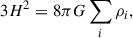
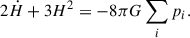
where a(t) denotes the scale factor and dΩ2 = dθ2 + sin2θ dϕ2. Substituting this metric into Eq. (2) yields the Friedmann equations:
 (5)
(5)
 (6)
(6)
Here, H = ȧ/a is the Hubble parameter and ρi and pi are the energy density and pressure of the ith cosmic component, respectively.
The conservation of the total energy-momentum tensor,  , leads to the continuity equation
 (7)
(7)
where wi = pi/ρi is the EoS parameter.
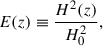
For non-relativistic matter (wm = 0), Eq. (7) gives ρm = ρm0a−3, while for DE characterized by wDE = −1, the density remains constant: ρDE = ρDE, 0. Consequently, the dimensionless Hubble function,
 (8)
(8)
is expressed as
 (9)
(9)
where Ωi = (8πGρi0)/(3H02) denotes the present density parameter of each component.
2.2. Dark energy parametrizations
While the ΛCDM model assumes a constant vacuum energy (w = −1), theoretical and observational considerations suggest that there are scenarios in which the DE EoS varies with time. For a general EoS w(z), the DE density evolves according to
![Mathematical equation: $$ \begin{aligned} f_{\mathrm{DE} }(z) = \exp \!\left[ 3 \int _0^z \frac{1 + w(z\prime )}{1 + z\prime } \, dz\prime \right]. \end{aligned} $$](/articles/aa/full_html/2026/05/aa57820-25/aa57820-25-eq11.gif) (10)
(10)
If w is constant, Eq. (10) yields fDE(z) = (1 + z)3(1 + w), i.e. the w cold dark matter (wCDM) model.
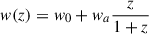
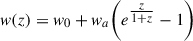
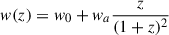
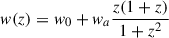
To capture possible time evolution, we considered the following EoS parametrizations:
-
Chevallier-Polarski-Linder (CPL) (Chevallier & Polarski 2001; Linder 2003):
-
The logarithmic model (Efstathiou 1999; Silva et al. 2012):

-
The exponential model (Najafi et al. 2024):
-
Jassal-Bagla-Padmanabhan (JBP) (Jassal et al. 2005):
-
Barboza-Alcaniz (BA) (Barboza & Alcaniz 2008):
-
Generalized Emergent DE (GEDE) (Li & Shafieloo 2020):
![Mathematical equation: $$ { w}(z) = -1 - \frac{\Delta }{3\ln 10} \left[ 1 + \tanh \!\left( \Delta \log _{10}\!\frac{1+z}{1+z_t} \right) \right], $$](/articles/aa/full_html/2026/05/aa57820-25/aa57820-25-eq17.gif)
where Δ is the free parameter and zt is a derived parameter, denoting the redshift at which the matter and DE densities become equal, ρm(zt) = ρDE(zt), implying Ωm0(1 + zt)3 = ΩDE(zt).
Given any of the w(z) above, fDE(z) follows from Eq. (10); inserting this into Eq. (9) yields the corresponding expansion history, E(z).
2.3. Non-flat universe extensions
Although the ΛCDM model assumes spatial flatness, several recent analyses suggest that the cosmic curvature may deviate slightly from zero. Planck data indicate a mild preference for a closed universe (Aghanim et al. 2020; Handley 2021; Di Valentino et al. 2020), while low-redshift probes lean towards an open geometry (Wu & Zhang 2025). These tensions motivated us to consider non-flat cosmologies.
2.3.1. Non-flat ΛCDM
Incorporating a curvature component, the dimensionless expansion rate becomes
 (11)
(11)
where Ωk quantifies the present curvature contribution.
2.3.2. Non-flat wCDM
If DE has a constant EoS of w ≠ −1, the corresponding expansion rate generalizes to
 (12)
(12)
This model highlights the degeneracy between curvature and the DE EoS parameter, emphasizing the importance of including Ωk when constraining cosmic acceleration.
3. Dataset and methodology
We performed parameter estimation and obtained observational constraints on the free parameters of each DE model proposed in Section 2. We now discuss the implications of these models further. To explore the parameter space, we used the Metropolis–Hastings MCMC sampling (Hastings 1970), integrated with the cosmological inference code Cobaya (Torrado & Lewis 2021). The theoretical models were computed using the Einstein–Boltzmann solver CAMB (Lewis et al. 2000). The convergence of the MCMC chains was tested using the Gelman-Rubin statistic (R − 1) (Gelman & Rubin 1992), adopting R − 1 < 0.01 as the threshold for convergence. The MCMC results were subsequently analysed and visualized using the GetDist package (Lewis 2025).
We applied the Bayesian evidence selection criterion using the publicly available code MCEvidence (Heavens et al. 2017a,b), which provides an estimate of the marginal likelihood for each cosmological model given the observational data. This allows a direct comparison between two competing models (i and j) through the Bayes factor defined as Bij ≡ Zi/Zj or, equivalently, in logarithmic form: lnBij = lnZi − lnZj. A positive value of lnBij indicates a preference for model i over model j.
To interpret the strength of the evidence, we adopted the revised Jeffreys scale (Kass & Raftery 1995; Trotta 2008). According to this criterion, |lnBij|< 1 corresponds to inconclusive evidence, 1 ≤ |lnBij|< 2.5 indicates weak evidence, 2.5 ≤ |lnBij|< 5 corresponds to moderate evidence, 5 ≤ |lnBij|< 10 indicates strong evidence, and |lnBij|≥10 is considered decisive evidence in favour of one model over the other.
For parameter estimation, we used the Lyα BAO measurements from DESI DR2 and the galaxy BAO measurements from DR2, the SN Ia sample, and the CamSpec CMB likelihood, which are listed below.
-
Lyα forest BAO. We used the Lyα forest BAO measurement from the DR2, which provides constraints on the distance ratios DH(zeff)/rd = 8.63 ± 0.10 and DM(zeff)/rd = 38.98 ± 0.53 at the effective redshift zeff = 2.33, with a correlation coefficient of ρ = −0.43.
-
DESI DR2 galaxy BAO. In addition to the Lyα forest BAO measurement, we also used the galaxy clustering BAO data from DESI DR2 (Abdul Karim et al. 2025). This sample provides measurements of DM/rd and DH/rd in five redshift bins covering the 0.5 < z < 1.5 range, as well as a single isotropic BAO constraint at z = 0.295.
-
Type Ia supernovae: We also used the unanchored SN Ia sample from Brout et al. (2022), which consists of 1701 light curves from 1550 SNe Ia. In our analysis, we excluded supernovae with redshifts of z < 0.01 as such low-redshift data are affected by significant systematic uncertainties arising from peculiar velocities. Then, we used the recalibrated 1820 photometric light curves from DES-Dovekie (Popovic et al. 2025), which includes 1623 DES-discovered SN Ia and 197 externally sourced low-z supernovae from the Center for Astrophysics (CfA) and Carnegie Supernova Project (CSP) samples (Hicken et al. 2009, 2012; Foley 2017). The revised DES-Dovekie has 1718 SNe Ia that are also included in DES-SN5YR (Vincenzi et al. 2024). We also used the Union3 compilation (Rubin et al. 2025), which contains 2087 SNe Ia, including 1363 that overlap with Pantheon+, providing complementary redshift coverage. For all supernova datasets, we marginalized over the absolute magnitude parameter (M) to account for calibration uncertainties (see Equations (A9)–(A12) in Goliath et al. 2001).
-
CMB CamSpec likelihood: Finally, we used the temperature (TT), polarization (EE), and cross-correlation (TE) power spectra measured by Planck. For the large angular scales (ℓ < 30), we used the Commander and SimAll likelihoods, while for smaller scales (ℓ ≥ 30) we used the CamSpec likelihood (Efstathiou & Gratton 2020; Rosenberg et al. 2022). The CamSpec is a new likelihood based on the latest Planck PR4 Next-generation Planck Iterative Processing Environment (NPIPE) data release, replacing the earlier Plik likelihood derived from the PR3 release. In addition, we used the CMB lensing measurements obtained from the joint analysis of Planck and Atacama Cosmology Telescope (ACT) Data Release 6 (DR6) data (Madhavacheril et al. 2024).
The priors chosen for these models are summarized in Table 1.
Priors on the cosmological parameters used in the analysis.
4. Results
In Fig. 1, we show the corner plot obtained by superimposing each model considered in this paper. The off-diagonal panels show the 2D marginalized confidence contours at the 68% and 95% confidence levels, while the diagonal panels show the 1D marginalized posterior distributions for each parameter. Fig. 2 shows the 2D marginalized confidence contours at the 1σ and 2σ confidence levels for the different cosmological models. In this analysis, we used the parameter values predicted by the ΛCDM model for each combination of datasets, treating it as the baseline model for comparison. In cosmology, we rely on observation-based inference, with which it is not possible to repeat measurements under identical conditions to achieve the same degree of precision. For this reason, evidence at the level of 2–4σ is generally considered significant. Several well-known anomalies such as the Hubble tension, the S8 tension, the MB calibration tension, and the CMB lensing anomaly are discussed as ‘tensions’ precisely because they appear within this range. Therefore, we quantified the deviation of each model parameter from the ΛCDM baseline in terms of the tension (T), defined as 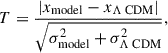 where xmodel and xΛCDM are the predicted parameter values (e.g. H0, Ωm, etc.), and σmodel and σΛCDM are their uncertainties (Camera et al. 2019; Chang et al. 2019). The results are interpreted using the following scale: |T|< 1σ, which is consistent with ΛCDM; 1σ ≤ |T|< 2.5σ, which is consistent with inconclusive tension; 2.5σ ≤ |T|< 5σ, which is consistent with moderate tension; 5σ ≤ |T|< 10σ, which is consistent with strong tension; and |T|≥10σ, which is consistent with decisive tension.
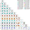 |
Fig. 1. Corner plot obtained by superimposing the ΛCDM, oΛCDM, wCDM, owCDM, CPL, logarithmic, exponential, JBP, BA, and GEDE models using DESI DR2 Lyα forest measurements in combination with the CMB, galaxy BAO, and SN Ia (Pantheon+, DES-Dovekie, and Union3) datasets. The contours correspond to the 68% (1σ) and 95% (2σ) confidence levels. The cross symbols indicate parameters that are not present in the corresponding models. |
First, we compared the predicted values of H0 for each model with those obtained from the ΛCDM model across different dataset combinations. The level of tension depends both on the DE parametrization and the dataset considered. For the Lyα + CMB + Galaxy BAO combination, the CPL, logarithmic, exponential, BA, wCDM, JBP, and GEDE models show inconclusive evidence of tension with respect to the ΛCDM prediction for H0, with deviations in the range 1σ ≲ |T|≲2.5σ. In contrast, the open Λ cold dark matter (oΛCDM) and open w cold dark matter (owCDM) models remain consistent with ΛCDM. For the Lyα + CMB + Pantheon+ and Lyα + CMB + DES-Dovekie combinations, all considered DE models remain consistent with the ΛCDM prediction for H0, as the corresponding tension values satisfy |T|< 1σ. Finally, for Lyα + CMB + Union3, the wCDM, owCDM, JBP, and GEDE models show inconclusive evidence of tension with respect to ΛCDM, whereas the remaining parametrizations remain consistent with the baseline model.
Now, Figs. 2a, b, and c show the 2D marginalized confidence contours in the {103Ωk − Ωm}, {w − Ωm}, and {103Ωk − w} planes for the oΛCDM, wCDM, and owCDM models, respectively. First, we discuss the constraints on the curvature parameter, Ωk. Since the numerical values of the curvature parameter are very close to zero, we constrained Ωk in the analysis, but we present the results in terms of 103Ωk for better visualization. For the oΛCDM model, the curvature parameter is predicted to be 103Ωk = 2.2 ± 1.1 and  for the Lyα + CMB + Galaxy BAO and Lyα + CMB + Pantheon+ dataset combinations, respectively. When combined with DES-Dovekie and Union3, the oΛCDM model predicts
  and
and  , respectively. Similarly, for the owCDM model, the curvature parameter is predicted to remain close to zero for all dataset combinations, with 103Ωk = 2.0 ± 1.2, 103Ωk = −1.8 ± 2.8, 103Ωk = −1.9 ± 2.8, and
  for the Lyα + CMB + Galaxy BAO, Lyα + CMB + Pantheon+, Lyα + CMB + DES-Dovekie, and Lyα + CMB + Union3 dataset combinations, respectively. All these results remain fully consistent with a spatially flat Universe (Ωk = 0) and are also in close agreement with previous measurements from Wilkinson Microwave Anisotropy Probe (WMAP) (−0.0179 < Ωk < 0.0081, 95% CL) (Bennett et al. 2013), Balloon Observations Of Millimetric Extragalactic Radiation and Geophysics (BOOMERanG) (0.988 < ΩM/R + ΩΛ < 1.0081, 95% CL) (de Bernardis et al. 2000), and Planck (ΩM/R + ΩΛ = 1.00 ± 0.026, 68% CL) (Aghanim et al. 2020). Further, the wCDM model predicts w = −1.046 ± 0.036 when the Lyα data are combined with the CMB and Galaxy BAO samples, whereas when Lyα is combined with the CMB and different SN Ia samples, it predicts w > −1.
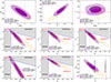 |
Fig. 2. 2D marginalized confidence contours of different planes of the oΛCDM, wCDM, owCDM, CPL, logarithmic, exponential, JBP, BA, and GEDE models using DESI DR2 Lyα forest measurements in combination with the CMB, galaxy BAO, and SN Ia (Pantheon+, DES-Dovekie, and Union3) measurements at 68% (1σ) and 95% (2σ) confidence intervals. |
Figs. 2d, e, f, g, and h show the 2D marginalized confidence contours at the 1σ and 2σ confidence levels in the {w0 − wa} plane for the CPL, logarithmic, exponential, JBP, and BA models, respectively. All models predict w0 > −1 and wa < 0 when the Lyα data are combined with the CMB, different SN Ia samples (Pantheon+, DES-Dovekie, and Union3), and Galaxy BAO, indicating a preference for the DE scenario characterized by w0 > −1, wa < 0, and w0 + wa < −1, namely the Quintom-B scenario (Cai et al. 2026; Ye et al. 2025), in which the EoS parameter satisfies w < −1 in the past and evolves to w > −1 at the present epoch. By crossing w = −1, this behaviour corresponds to a phantom crossing (Silva & Nunes 2025).
Fig. 2i shows the 2D marginalized confidence contours in the {Δ − Ωm} plane for the GEDE model. We find that the GEDE model predicts Δ = 0.36 ± 0.26 when the Lyα data are combined with the CMB and Galaxy BAO samples, showing an inconclusive deviation from the ΛCDM model. However, when different SN Ia samples (Pantheon+, DES-Dovekie, and Union3) are included, the GEDE model yields negative values of Δ, indicating a possible injection of DE at high redshifts (Lodha et al. 2025a,b).
In Fig. 3, we present a radar plot showing the deviations of the oΛCDM, wCDM, owCDM, CPL, logarithmic, exponential, JBP, BA, and GEDE models relative to the ΛCDM model. The deviations are quantified using the Nσ analysis based on the differences in the minimum χ2 values, which are defined as ΔχMAP2 ≡ χModel2 − χΛCDM2. As our main goal was to assess the preference for dynamical DE over the ΛCDM model, we focus on the CPL, logarithmic, exponential, JBP, BA, and GEDE models in our further discussion. Since ΛCDM is a special case of the dynamical DE model, the statistic ΔχMAP2 is expected to follow a χ2 distribution, with degrees of freedom equal to the number of additional parameters in the extended model, assuming Gaussian errors and that the null hypothesis (ΛCDM) is valid. For easier interpretation, we converted ΔχMAP2 into an equivalent frequentist significance (Nσ) for a 1D Gaussian distribution, CDFχ2(ΔχMAP2 | k d.o.f.)
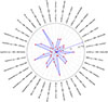 |
Fig. 3. Radar plot showing the deviation of the oΛCDM, wCDM, owCDM, CPL, logarithmic, exponential, JBP, BA, and GEDE models in terms of σ. Each radial distance, ending at a red dot, represents the statistical significance of the deviation. The radial axes correspond to the different dataset combinations, which are labelled along the outer edge of the plot. |
For the Lyα + CMB + Galaxy BAO combination, the CPL model shows moderate preference (≃3.10σ) relative to ΛCDM, while the logarithmic, exponential, and BA models also show moderate preference at the ∼2.6–2.8σ level. The JBP and GEDE models show an inconclusive preference (≃2.10σ and ≃1.72σ, respectively) relative to ΛCDM. For the Lyα + CMB + Pantheon+ dataset, all dynamical DE models remain statistically consistent with ΛCDM, with deviations close to or slightly above 1σ. The largest deviation arises for the GEDE model (≃1.09σ), which only corresponds to an inconclusive preference. For the Lyα + CMB + DES-Dovekie combination, all models remain statistically consistent with ΛCDM, with deviations below ∼1.3σ. The JBP model shows the largest deviation (≃1.21σ), which still lies within the range of inconclusive preference, while the GEDE model shows no deviation from ΛCDM. Finally, for the Lyα + CMB + Union3 combination, the CPL model shows inconclusive preference (≃2.02σ); the remaining models also fall within the range of inconclusive preference, with deviations in the ∼1.2–1.8σ range relative to ΛCDM.
Based on the logarithmic form of the Bayes factor, |lnBi, j|, and following the revised Jeffreys scale, we obtained the following results. For the Lyα + CMB + Galaxy BAO combination, the wCDM and owCDM models show moderate evidence against ΛCDM, while the oΛCDM, CPL, JBP, and GEDE models provide weak evidence. In contrast, the logarithmic, exponential, and BA models yield inconclusive evidence relative to the ΛCDM baseline. For the Lyα + CMB + Pantheon+ combination, the owCDM model shows strong evidence against ΛCDM, whereas the oΛCDM, wCDM, CPL, logarithmic, exponential, JBP, BA, and GEDE models show moderate evidence. For the Lyα + CMB + DES-Dovekie dataset, the owCDM model again shows strong evidence against ΛCDM. The oΛCDM, wCDM, CPL, logarithmic, exponential, BA, and GEDE models provide moderate evidence, while the JBP model shows weak evidence. Finally, for the Lyα + CMB + Union3 combination, the oΛCDM and owCDM models provide moderate evidence against ΛCDM. The wCDM, exponential, logarithmic, CPL, BA, JBP, and GEDE models also show moderate evidence relative to the ΛCDM prediction.
5. Discussion and conclusions
In this work, we investigated the cosmological implications of the DESI DR2 Lyα forest measurements in combination with several datasets, including the CMB, Galaxy BAO, and multiple SN Ia compilations (Pantheon+, DES-Dovekie, and Union3), to test the preference of the dynamical DE model over the ΛCDM model. Using various redshift-dependent DE parametrizations (CPL, logarithmic, exponential, JBP, BA, and GEDE models), as well as constant EoS and non-flat extensions, we performed a comprehensive Bayesian analysis based on the Metropolis–Hastings MCMC algorithm implemented in Cobaya. The theoretical predictions were computed using the Einstein–Boltzmann solver CAMB. Model comparison was carried out using the Bayesian evidence computed with MCEvidence, interpreted through the revised Jeffreys scale. Our main results can be summarized as follows:
-
Hubble and matter density parameters. The inclusion of DESI DR2 Lyα measurements together with other cosmological datasets shows dataset-dependent variations in both the Hubble constant,H0, and the matter density parameter, Ωm. In particular, the Lyα + CMB + Galaxy BAO combination shows the largest deviations from the ΛCDM predictions. For this dataset combination, several DE parametrizations, including the CPL, logarithmic, exponential, BA, wCDM, JBP, and GEDE models, show inconclusive evidence of tension with respect to the ΛCDM prediction for both H0 and Ωm, with deviations typically in the 1σ ≲ |T|≲2.5σ range. In contrast, the oΛCDM and owCDM models remain statistically consistent with ΛCDM.
-
Spatial curvature. The non-flat extensions oΛCDM and owCDM yield curvature constraints consistent with Ωk ≈ 0, with all dataset combinations providing tightly constrained values of Ωk that are statistically consistent with zero. These findings support the assumption of a spatially flat Universe, in agreement with previous results from WMAP, BOOMERanG, and Planck.
-
Quintom-B scenario. All redshift-dependent models (CPL, logarithmic, exponential, JBP, and BA) predict values of w0 > −1 and wa < 0, as indicated by the 2D marginalized confidence contours at the 1σ and 2σ confidence levels in the {w0 − wa} plane. These results show that the DE scenario is characterized by a Quintom-B type (w0 > −1, wa < 0, and w0 + wa < −1) in which the EoS parameter satisfies w < −1 in the past and evolves to w > −1 at the present epoch by crossing the phantom divide, w = −1, rather than a cosmological constant model in which DE is characterized by w = −1.
-
Evidence for dynamical DE. The inclusion of Lyα data in the combined cosmological analysis shows that the agreement with the ΛCDM model depends strongly on the choice of DE parametrization and dataset combination. For the Lyα + CMB + Galaxy BAO dataset, the CPL model shows moderate preference relative to ΛCDM (∼3.10σ), while the logarithmic, exponential, and BA models also exhibit a moderate preference (∼2.6–2.8σ). The JBP and GEDE models only show an inconclusive preference. When Lyα is combined with CMB and Pantheon+ or DES-Dovekie, all models remain statistically consistent with ΛCDM. For the Lyα + CMB + Union3 combination, the CPL model shows only an inconclusive preference, while the remaining parametrizations remain broadly compatible with the ΛCDM prediction.
-
Bayesian model comparison. Based on the Bayesian evidence and the revised Jeffreys scale, the preference for dynamical DE models relative to ΛCDM depends strongly on the dataset combination. For the Lyα + CMB + Galaxy BAO dataset, wCDM and owCDM show moderate evidence, while most other models provide weak or inconclusive evidence. When combined with Pantheon+ or DES-Dovekie, the owCDM model shows strong evidence against ΛCDM, whereas the remaining models generally yield moderate evidence.
Our results indicate that when high-redshift DESI DR2 Lyα forest measurements are combined with other cosmological datasets, the level of agreement with the ΛCDM model becomes strongly dependent on the adopted DE parametrization and dataset combination. For the Lyα + CMB + Galaxy BAO dataset, deviations from ΛCDM reach the ∼1.7–3.10σ level for several dynamical DE models, while the logarithmic, exponential, and BA parametrizations show a moderate preference at the ∼2.6–2.8σ level. When different SN Ia samples are included, the deviations decrease significantly and remain typically below ∼2σ, indicating only an inconclusive preference relative to ΛCDM. Although these deviations are not statistically decisive, they highlight the sensitivity of cosmological constraints to high-redshift Lyα measurements and suggest that future high-precision observations such as those in DESI Data Release 3 may provide further insight into the nature of DE.
The upcoming Stage IV surveys will shed new light on the nature of DE. DESI will deliver additional DR2 constraints from full-shape fitting, bispectrum, and gravitational lensing in 2025–2026, followed by DR3 BAO results expected in 2027; this will provide new insights into the state of DE, the ΛCDM model, and the phantom crossing. Observations from the Hubble Space Telescope and James Webb Space Telescope will refine H0, while the Simons Observatory (Ade et al. 2019), Legacy Survey of Space and Time (LSST) at the Vera C. Rubin Observatory (Ade et al. 2019), and ESA’s Euclid mission (Laureijs et al. 2011) will soon provide new CMB, weak lensing, and supernova data. The Subaru Prime Focus Spectrograph (PFS) survey (Takada et al. 2014) and the Nancy Grace Roman Space Telescope (Spergel et al. 2015) will extend DE constraints beyond z > 1, and in the 2030s DESI-II (Dawson et al. 2022) will push these boundaries even further. If Stage IV surveys challenge the standard ΛCDM model, the next questions will concern how we move forward, which new observing methods or cross-survey approaches we should focus on first, and whether there any particular signals or patterns in the data that could point us towards the true nature of DE. These will not be easy questions to answer. In the long run, we may find that proving ΛCDM is incomplete was the simple part and that understanding what actually drives cosmic acceleration is a much harder task.
Acknowledgments
SC acknowledges the Istituto Nazionale di Fisica Nucleare (INFN) Sez. di Napoli, Iniziative Specifiche QGSKY and MoonLight-2 and the Istituto Nazionale di Alta Matematica (INdAM), gruppo GNFM, for the support. This paper is based upon work from COST Action CA21136 Addressing observational tensions in cosmology with systematics and fundamental physics (CosmoVerse), supported by COST (European Cooperation in Science and Technology). The authors would like to thank Prof. Ravi Kumar Arya, Director of the Xiangshan 5G/6G Laboratory, Zhongshan Institute of Changchun University of Science and Technology, China, for providing access to the HPC facility for the MCMC analysis performed in this work.
References
- Abdul Karim, M., Aguilar, J., Ahlen, S., et al. 2025, Phys. Rev. D, 112, 083515 [Google Scholar]
- Adame, A., Aguilar, J., Ahlen, S., et al. 2025a, JCAP, 2025, 124 [CrossRef] [Google Scholar]
- Adame, A. G., Aguilar, J., Ahlen, S., et al. 2025b, JCAP, 02, 021 [CrossRef] [Google Scholar]
- Ade, P., Aguirre, J., Ahmed, Z., et al. 2019, JCAP, 2019, 056 [Google Scholar]
- Aghanim, N., Akrami, M., Ashdown, J., et al. 2020, A&A, 641, A6 [NASA ADS] [CrossRef] [EDP Sciences] [Google Scholar]
- Alam, S., & Hossain, M. W. 2025, ArXiv e-prints [arXiv:2510.03779] [Google Scholar]
- Barboza, E., Jr, & Alcaniz, J. 2008, Phys. Lett. B, 666, 415 [Google Scholar]
- Bennett, C. L., Larson, D., Weiland, J. L., et al. 2013, ApJS, 208, 20 [Google Scholar]
- Bernardo, R. C., Grandón, D., Said Levi, J., & Cárdenas, V. H. 2022, Phys. Dark Univ., 36, 101017 [Google Scholar]
- Brout, D., Scolnic, D., Popovic, B., et al. 2022, ApJ, 938, 110 [NASA ADS] [CrossRef] [Google Scholar]
- Cai, Y., Ren, X., Qiu, T., Li, M., & Zhang, X. 2026, Natl (Rev: Sci) [Google Scholar]
- Camera, S., Martinelli, M., & Bertacca, D. 2019, Phys. Dark Univ., 23, 100247 [NASA ADS] [CrossRef] [Google Scholar]
- Capozziello, S., Sarracino, G., & Spallicci, A. D. A. M. 2023, Phys. Dark Univ., 40, 101201 [Google Scholar]
- Chang, C., Wang, M., Dodelson, S., et al. 2019, MNRAS, 482, 3696 [Google Scholar]
- Chevallier, M., & Polarski, D. 2001, Int. J. Mod. Phys. D, 10, 213 [Google Scholar]
- Choudhury, S. R. 2025, ApJ, 986, L31 [Google Scholar]
- Choudhury, S. R., & Okumura, T. 2024, ApJ, 976, L11 [NASA ADS] [CrossRef] [Google Scholar]
- Choudhury, S. R., Okumura, T., & Umetsu, K. 2025, ApJ, 994, L26 [Google Scholar]
- Colgáin, E. Ó., Sheikh-Jabbari, M. M., & Yin, L. 2021, Phys. Rev. D, 104, 023510 [CrossRef] [Google Scholar]
- Colgáin, E. Ó., Pourojaghi, S., & Sheikh-Jabbari, M. M. 2025, Galaxies, 13, 133 [Google Scholar]
- Colgáin, E. Ó., Pourojaghi, S., Sheikh-Jabbari, M. M., & Yin, L. 2026, Phys. Dark Univ., 52, 102268 [Google Scholar]
- Cuceu, A., Font-Ribera, A., Nadathur, S., Joachimi, B., & Martini, P. 2023, Phys. Rev. Lett., 130, 191003 [NASA ADS] [CrossRef] [Google Scholar]
- Cuceu, A., Herrera-Alcantar, H. K., Gordon, C., et al. 2025, ArXiv e-prints [arXiv:2509.15308] [Google Scholar]
- Dawson, K., Hearin, A., Heitmann, K., et al. 2022, ArXiv e-prints [arXiv:2203.07291] [Google Scholar]
- de Bernardis, P., Ade, P. A., Bock, J. J., et al. 2000, Nature, 404, 955 [NASA ADS] [CrossRef] [Google Scholar]
- Delubac, T., Rich, J., Bailey, S., et al. 2013, A&A, 552, A96 [NASA ADS] [CrossRef] [EDP Sciences] [Google Scholar]
- Demianski, M., Piedipalumbo, E., Sawant, D., & Amati, L. 2018, Mem. Soc. Astron. It., 89, 197 [Google Scholar]
- Des Bourboux, H. D. M., Rich, J., Font-Ribera, A., et al. 2020, ApJ, 901, 153 [CrossRef] [Google Scholar]
- Di Valentino, E., Melchiorri, A., & Silk, J. 2020, Nat. Astron., 4, 196 [Google Scholar]
- Di Valentino, E., Said, J. L., Riess, A., et al. 2025, Phys. Dark Univ., 49, 101965 [Google Scholar]
- Dinda, B. R., Maartens, R., & Clarkson, C. 2025, JCAP, 12, 025 [Google Scholar]
- Efstathiou, G. 1999, MNRAS, 310, 842 [Google Scholar]
- Efstathiou, G., & Gratton, S. 2020, MNRAS, 496, L91 [Google Scholar]
- Foley, R. 2017, Keck Observatory Archive, U079, 39 [Google Scholar]
- Gelman, A., & Rubin, D. B. 1992, Stat. Sci., 7, 457 [Google Scholar]
- Goliath, M., Amanullah, R., Astier, P., Goobar, A., & Pain, R. 2001, A&A, 380, 6 [NASA ADS] [CrossRef] [EDP Sciences] [Google Scholar]
- Handley, W. 2021, Phys. Rev. D, 103, L041301 [NASA ADS] [CrossRef] [Google Scholar]
- Hastings, W. K. 1970, Biometrika, 57, 97 [Google Scholar]
- Heavens, A., Fantaye, Y., Mootoovaloo, A., et al. 2017a, ArXiv e-prints [arXiv:1704.03472] [Google Scholar]
- Heavens, A., Fantaye, Y., Sellentin, E., et al. 2017b, Phys. Rev. Lett., 119, 101301 [Google Scholar]
- Hicken, M., Challis, P., Jha, S., et al. 2009, ApJ, 700, 331 [Google Scholar]
- Hicken, M., Challis, P., Kirshner, R. P., et al. 2012, ApJS, 200, 12 [Google Scholar]
- Högås, M., & Mörtsell, E. 2025, Phys. Rev. D, 112, 103515 [Google Scholar]
- Jassal, H., Bagla, J., & Padmanabhan, T. 2005, MNRAS, 356, L11 [Google Scholar]
- Jiang, J.-Q., Pedrotti, D., da Costa, S. S., & Vagnozzi, S. 2024, Phys. Rev. D, 110, 123519 [Google Scholar]
- Kass, R. E., & Raftery, A. E. 1995, J. Am. Stat. Assoc., 90, 773 [Google Scholar]
- Laureijs, R., Amiaux, J., Arduini, S., et al. 2011, ArXiv e-prints [arXiv:1110.3193] [Google Scholar]
- Lee, S. 2026, Ann. Phys., 489, 170453 [Google Scholar]
- Lewis, A. 2025, JCAP, 2025, 025 [Google Scholar]
- Lewis, A., Challinor, A., & Lasenby, A. 2000, ApJ, 538, 473 [Google Scholar]
- Li, X., & Shafieloo, A. 2020, ApJ, 902, 58 [NASA ADS] [CrossRef] [Google Scholar]
- Linder, E. V. 2003, Phys. Rev. Lett., 90, 091301 [Google Scholar]
- Liu, T., Li, X., Xu, T., Biesiada, M., & Wang, J. 2025, Eur. Phys. J. C, 85, 1351 [Google Scholar]
- Lodha, K., Calderon, R., Matthewson, W. L., et al. 2025a, Phys. Rev. D, 112, 083511 [Google Scholar]
- Lodha, K., Shafieloo, A., Calderon, R., et al. 2025b, Phys. Rev. D, 111, 023532 [Google Scholar]
- Lovelock, D. 1971, J. Math. Phys., 12, 498 [CrossRef] [Google Scholar]
- Madhavacheril, M. S., Qu, F. J., Sherwin, B. D., et al. 2024, ApJ, 962, 113 [CrossRef] [Google Scholar]
- Najafi, M., Pan, S., Di Valentino, E., & Firouzjaee, J. T. 2024, Phys. Dark Univ., 45, 101539 [Google Scholar]
- Odintsov, S. D., Sáez-Chillón Gómez, D., & Sharov, G. S. 2025, Eur. Phys. J. C, 85, 298 [Google Scholar]
- Odintsov, S. D., Oikonomou, V. K., & Sharov, G. S. 2026, JHEAp, 50, 100471 [Google Scholar]
- Pedrotti, D., Escamilla, L. A., Marra, V., Perivolaropoulos, L., & Vagnozzi, S. 2026, Phys. Rev. D, 113, 043507 [Google Scholar]
- Popovic, B., Shah, P., Kenworthy, W., et al. 2025, ArXiv e-prints [arXiv:2511.07517] [Google Scholar]
- Rosenberg, E., Gratton, S., & Efstathiou, G. 2022, MNRAS, 517, 4620 [NASA ADS] [CrossRef] [Google Scholar]
- Rubin, D., Aldering, G., Betoule, M., et al. 2025, ApJ, 986, 231 [Google Scholar]
- Silva, E., & Nunes, R. C. 2025, JCAP, 2025, 078 [Google Scholar]
- Silva, R., Goncalves, R., Alcaniz, J., & Silva, H. 2012, A&A, 537, A11 [Google Scholar]
- Slosar, A., Iršič, V., Kirkby, D., et al. 2013, JCAP, 2013, 026 [CrossRef] [Google Scholar]
- Spergel, D., Gehrels, N., Baltay, C., et al. 2015, ArXiv e-prints [arXiv:1503.03757] [Google Scholar]
- Takada, M., Ellis, R. S., Chiba, M., et al. 2014, PASJ, 66, R1 [Google Scholar]
- Torrado, J., & Lewis, A. 2021, JCAP, 2021, 057 [Google Scholar]
- Trotta, R. 2008, Contemp. Phys., 49, 71 [Google Scholar]
- Vagnozzi, S. 2020, Phys. Rev. D, 102, 023518 [Google Scholar]
- Vagnozzi, S. 2023, Universe, 9, 393 [NASA ADS] [CrossRef] [Google Scholar]
- Vincenzi, M., Brout, D., Armstrong, P., et al. 2024, ApJ, 975, 86 [NASA ADS] [CrossRef] [Google Scholar]
- Wu, P. J., & Zhang, X. 2025, Phys. Rev. D, 112, 063514 [Google Scholar]
- Ye, G., Martinelli, M., Hu, B., & Silvestri, A. 2025, Phys. Rev. Lett., 134, 181002 [Google Scholar]
Appendix A: Additional tables
Tables A.1 and A.2 present the mean values of the cosmological parameters for each model, together with their 68% (1σ) confidence levels.
Numerical values of cosmological parameters at 68% confidence level for different dataset combinations.
Numerical values of cosmological parameters at 68% confidence level for different dataset combinations.
All Tables
Numerical values of cosmological parameters at 68% confidence level for different dataset combinations.
Numerical values of cosmological parameters at 68% confidence level for different dataset combinations.
All Figures
|
Fig. 1. Corner plot obtained by superimposing the ΛCDM, oΛCDM, wCDM, owCDM, CPL, logarithmic, exponential, JBP, BA, and GEDE models using DESI DR2 Lyα forest measurements in combination with the CMB, galaxy BAO, and SN Ia (Pantheon+, DES-Dovekie, and Union3) datasets. The contours correspond to the 68% (1σ) and 95% (2σ) confidence levels. The cross symbols indicate parameters that are not present in the corresponding models. |
| In the text | |
|
Fig. 2. 2D marginalized confidence contours of different planes of the oΛCDM, wCDM, owCDM, CPL, logarithmic, exponential, JBP, BA, and GEDE models using DESI DR2 Lyα forest measurements in combination with the CMB, galaxy BAO, and SN Ia (Pantheon+, DES-Dovekie, and Union3) measurements at 68% (1σ) and 95% (2σ) confidence intervals. |
| In the text | |
|
Fig. 3. Radar plot showing the deviation of the oΛCDM, wCDM, owCDM, CPL, logarithmic, exponential, JBP, BA, and GEDE models in terms of σ. Each radial distance, ending at a red dot, represents the statistical significance of the deviation. The radial axes correspond to the different dataset combinations, which are labelled along the outer edge of the plot. |
| In the text | |
Current usage metrics show cumulative count of Article Views (full-text article views including HTML views, PDF and ePub downloads, according to the available data) and Abstracts Views on Vision4Press platform.
Data correspond to usage on the plateform after 2015. The current usage metrics is available 48-96 hours after online publication and is updated daily on week days.
Initial download of the metrics may take a while.