| Issue |
A&A
Volume 708, April 2026
|
|
|---|---|---|
| Article Number | A307 | |
| Number of page(s) | 7 | |
| Section | Cosmology (including clusters of galaxies) | |
| DOI | https://doi.org/10.1051/0004-6361/202556955 | |
| Published online | 17 April 2026 | |
Testing the cosmological principle with quasars
1
School of Physics and Technology, Xinjiang University, Urumqi 830046, China
2
School of Physics and Electronics, Henan University, Kaifeng 475004, China
3
Xinjiang Astronomical Observatory, Chinese Academy of Sciences, Urumqi 830011, China
4
School of Physics and Astronomy, China West Normal University, Sichuan 637002, China
★ Corresponding authors: This email address is being protected from spambots. You need JavaScript enabled to view it.
, This email address is being protected from spambots. You need JavaScript enabled to view it.
Received:
22
August
2025
Accepted:
9
March
2026
Abstract
The cosmological principle posits that the universe is homogeneous and isotropic on the large scales. In history, the cosmological principle was confirmed by various cosmological observations from CMB to large scale structure. However, several new challenges to the cosmological principle were reported in recent years, particularly in radio observations from overdispersed radio source counts to quasars. Here, we firstly present studies on the peculiar velocity of large-scale anisotropy by measuring the dipole signal from the DESI DR1 catalogue with a sample of 1 176 570 quasars (0.8 < z < 3.0). Our analysis reveals the peculiar velocity of |v| = 443.8 ± 204.1 km/s towards (l, b) = (107.4° ±86.8° ,28.4° ±45.2° ) in Galactic coordinates. The motion direction deviates from the CMB dipole (264.02°, 48.253°). The inferred velocity is consistent at the 1.56σ level with the value of 370 km/s from a purely kinematic interpretation of the CMB dipole. Based on the motion direction component analysis, we have not found any significant deviation from cosmological principle in current released quasars data.
Key words: quasars: general / large-scale structure of Universe
© The Authors 2026
 Open Access article, published by EDP Sciences, under the terms of the Creative Commons Attribution License (https://creativecommons.org/licenses/by/4.0), which permits unrestricted use, distribution, and reproduction in any medium, provided the original work is properly cited.
This article is published in open access under the Subscribe to Open model. This email address is being protected from spambots. You need JavaScript enabled to view it. to support open access publication.
1. Introduction
The Λ cold dark matter (ΛCDM) model, validated by decades of observational data, serves as the standard framework of modern cosmology. This model successfully reconciles the observed accelerated expansion of the Universe with the theory of general relativity, resting on two foundational pillars: the theory of gravity itself and the cosmological principle (CP).
The CP, a core postulate of the concordance ΛCDM model, posits that the Universe is statistically homogeneous and isotropic on scales larger than ∼100 Mpc. This assumption forms the basis of the standard Friedmann-Lemaître-Robertson-Walker (FLRW) cosmology.
Direct support for large-scale isotropy comes from the high degree of uniformity observed in the cosmic microwave background (CMB), which appears remarkably isotropic on small angular scales. Complementary evidence is provided by a variety of independent cosmological tracers, including large-scale galaxy surveys (Gibelyou & Huterer 2012; Sarkar et al. 2018; Franco et al. 2023), the X-ray background (Wu et al. 1999), the spatial distribution of galaxy clusters (Bengaly et al. 2016), radio galaxies (Blake & Wall 2002), and Type Ia supernovae (Gupta & Saini 2010; Sorrenti et al. 2023). Collectively, these observations robustly corroborate the statistical isotropy of the Universe on the largest observable scales.
Amidst this backdrop of large-scale isotropy, the CMB itself exhibits a hierarchy of anisotropies. It contains small-scale fluctuations at the level of approximately 1 part in 105, and a far more prominent dipole anisotropy of amplitude ∼1 part in 103 as measured in the heliocentric frame. Given its distinctive amplitude and dipolar pattern, this dominant signal is almost universally attributed to a kinematic effect–the peculiar motion of the Solar System relative to the CMB rest frame. The latest measurements infer a velocity of v = 369.825 ± 0.11 km/s towards the Galactic coordinates (l, b) = (264.021° ,48.253° ) (Hinshaw et al. 2009; Aghanim et al. 2020).
A critical test of the CP involves verifying the purely kinematic origin of the CMB dipole. This is achieved by measuring a corresponding dipole anisotropy in the distribution of distant matter. If the CP holds, the peculiar velocity inferred from the matter rest frame must be consistent with that derived from the CMB. The Ellis–Baldwin test provides a direct implementation of this idea (Ellis & Baldwin 1984). It posits that if the CMB dipole is indeed due to our motion through a homogeneous and isotropic universe, then a statistically congruent dipole must be present in the number counts of distant sources, such as radio galaxies. The velocity inferred from these counts should agree with the CMB-derived value. Consequently, under the CP, the large-scale distribution of matter should appear isotropic when viewed from the CMB rest frame. Any significant deviation would necessitate a physical explanation and could potentially challenge the validity of the CP itself.
However, this expectation has been challenged by several findings over the past two decades. Singal (2011) reported a significant discrepancy, finding the dipole amplitude from discrete radio sources to be approximately four times larger than that of the CMB, albeit with a possibly consistent direction. A congruent result was obtained by Rubart & Schwarz (2013) using the NVSS and WENSS surveys, who confirmed a dipole direction aligned with the CMB but an amplitude larger by a factor of approximately three. Extending the analysis to Type Ia supernovae, Singal (2022) similarly found a dipole amplitude about four times greater than the CMB value. In a distinct finding from the Pantheon+SH0ES supernova data, Sorrenti et al. (2023) reported a dipole amplitude consistent with the CMB but a direction differing with a statistical significance exceeding 3σ. Earlier, using the Union2.1 supernovae data, Yang et al. (2013) also found a preferred dipole direction via a dipole-fitting approach.
Secrest et al. (2021) used quasars (QSOs) from the CatWISE2020 catalogue and found a dipole direction offset by ∼27° from the CMB dipole, but with an amplitude over twice as large as expected, rejecting the kinematic interpretation at the 4.9σ level. Separately, Dam et al. (2023) also reported a significant tension through a Bayesian analysis of QSO data, measuring a dipole amplitude approximately 2.7 times larger than the kinematic expectation with a statistical significance of 5.7σ. Most recently, an analysis combining NVSS, RACS-low, and LoTSS-DR2 radio surveys reported a dipole amplitude 3.67 ± 0.49 times larger than the kinematic expectation, a 5.4σ discrepancy (Böhme et al. 2025). Secrest et al. (2022) further analysed radio galaxies and QSOs; they suggest that if the CMB dipole is assumed to be fully kinematic, the reference frames of these distant sources may exhibit an intrinsic anisotropy.
Other studies also hint at potential violations of statistical isotropy. For instance, isotropy tests performed on the SDSS Luminous Red Galaxy sample indicate a possible breakdown on scales as large as ∼300 h−1 Mpc (Park et al. 2017). In the CMB itself, a persistent hemispherical power asymmetry remains significant at an approximate the 3σ level in the latest data (Eriksen et al. 2004; Planck Collaboration VII 2020; Planck Collaboration XVI 2016). Notably, several of these anomalous signals, including the dipole in radio polarization and the alignment of the CMB low-order multipoles, indicate a preferred direction closely aligned with the CMB dipole (Ralston & Jain 2004). Furthermore, the discovery of enormous cosmic structures–such as large QSO groups (Clowes et al. 2013), correlated QSO orientations (Friday et al. 2022), and giant cosmic voids (Haslbauer et al. 2020; Keenan et al. 2013)–challenges the assumption of homogeneity at the largest scales.
The cumulative evidence from these diverse studies, which utilize different tracers and methodologies and sometimes yield conflicting results, calls into question the foundational assumption of large-scale isotropy and homogeneity inherent in the CP. In this context, we employed an independent cosmological probe to estimate the Solar System’s peculiar motion by analysing the dipole anisotropy in the sky distribution of QSO redshifts. The redshift dipole offers a direct measurement of the peculiar velocity relative to the matter reference frame traced by the QSOs. This method circumvents the need to account for local over- or under-densities (e.g. – a local void or specific clustering) and other large-scale structures (LSSs) known to potentially bias traditional number-count dipole measurements (Oayda et al. 2024; Rameez et al. 2018; Tiwari & Nusser 2016; Rubart et al. 2014).
This study aims to employ the high-precision, wide-coverage QSO data from the Dark Energy Spectroscopic Instrument (DESI) Data Release 1 (DR1) to perform a tomographic estimation of the dipole modulation across redshift bins, following the methodology of da Silveira Ferreira & Marra (2024). We used the DESI DR1 QSO sample to infer the Solar System’s peculiar velocity via the aberration effect, thereby performing a direct test of the CP through the Ellis–Baldwin test. This test confronts the kinematic dipole measured in the matter frame (traced by distant QSOs) with that of the cosmic rest frame (defined by the CMB).
This paper is structured as follows. Section 2 details the DESI and eBOSS QSO catalogues and their sky footprints used in the analysis. Section 3 presents the formalism for the redshift dipole, outlines the least-squares estimator used to measure the dipole amplitude, justifies the separate analysis of the northern Galactic caps (NGC) and the southern Galactic caps (SGC) to account for systematic depth variations, and introduces Fisher’s method for evaluating the overall statistical significance. Finally, Section 4 presents the main results and discusses their implications, concluding that the QSO dipole inferred from DESI DR1 is consistent with the kinematic interpretation of the CMB dipole, thereby finding no compelling evidence against the CP.
2. Data
We aim to test the CP using LSS tracers from recent spectroscopic surveys. To ensure robust results, we selected catalogues based on data quality, minimal known systematics, substantial sky coverage, and the ability to perform survey comparisons. Specifically, we utilized the final QSO clustering catalogues from the SDSS Extended Baryon Oscillation Spectroscopic Survey (eBOSS) and the early data release of the Dark Energy Spectroscopic Instrument (DESI). These catalogues provide observational weights, redshifts, and angular positions, and their derived cosmological parameters are consistent with the ΛCDM framework.
We analysed three distinct QSO samples:
(i) The eBOSS DR14 QSO Catalogue (Abolfathi et al. 2018): This catalogue contains 194 801 objects in the redshift range 0.04 < z < 6.95. After removing extreme outliers, 90% of the data lie within 0.42 < z < 3.28, leaving 192 853 objects. To mitigate potential boundary effects, we further restricted our analysis to the well-populated range 0.4 < z < 2.8, resulting in a final sample of 187 954 QSOs. The spectra cover the wavelength region 3610−10 140 Å at a spectral resolution in the range 1300 < R < 2500 (Abolfathi et al. 2018).
(ii) The eBOSS DR16 QSO Catalogue (Ross et al. 2020): This catalogue contains 343 708 QSOs with a tight and uniform redshift distribution in the range 0.8 < z < 2.2, selected from the final SDSS-IV/eBOSS quasar sample (Lyke et al. 2020). We used the entire specified range without further cuts. The spectra cover 3600−10 400 Å with a spectral resolution of R ∼ 2000 (Lyke et al. 2020). At the largest QSO sample at the time, eBOSS DR16 provided important data for cosmological analysis.
(iii) The DESI DR1 QSO Catalogue (DESI Collaboration 2025): The Dark Energy Spectroscopic Instrument (DESI) is a Stage IV spectroscopic survey designed to obtain tens of millions of galaxy and QSO redshifts to constrain dark energy and cosmological models (Adame et al. 2025). Its first data release (DR1) encompasses the first year of main survey observations. The public large-scale structure catalogue for QSOs contains 1 223 170 objects with confident redshift measurements in the range 0.8 < z < 3.5. The spectra cover the wavelength region 3600−9824 Å at a spectral resolution in the range 2000 < R < 5200 (DESI Collaboration 2025).
The construction of this LSS catalogue, detailed in Adame et al. (2025), involves critical steps to correct for systematic variations in the observed number density and to ensure its suitability for cosmological clustering analyses, as follows.
Systematic weights: The catalogue incorporates weights to correct for two main sources of spurious density fluctuations: (1) imaging systematics (e.g. seeing, depth, and stellar density) affecting the input target selection, and (2) variations in the ability to confidently measure redshifts from DESI spectra, which depend on observing conditions and instrumental performance.
Reference randoms: A matched set of synthetic ‘randoms’ is provided to accurately model the survey selection function, geometry, and fibre assignment incompleteness.
Validation: The two-point clustering measurements from the final LSS catalogue have been compared to high-fidelity simulations of the DESI survey. They are found to be in general statistical agreement, typically within a 2% factor in the inferred galaxy bias, confirming that observational systematic uncertainties are sub-dominant to statistical uncertainties for large-scale analyses.
For our dipole analysis, we used the total systematic weight wi provided in the catalogue, which combines the corrections mentioned above. To avoid potential biases from sparse edges of the redshift distribution, we restricted our analysis to the well-characterized range 0.8 < z < 3.0, yielding a final sample of 1 176 570 QSOs.
The redshift range and the total number of sources for each final sample are summarized in Table 1. The redshift distributions are visualized in Figure 1 as scatter plots with a bin width of Δz = 0.001
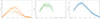 |
Fig. 1. Redshift distributions of the QSO catalogues. Left to right: eBOSS DR14 (orange), eBOSS DR16 (green), and DESI DR1 (blue). The DR14 distribution is broad (0.4 < z < 8) but sparse at the extremes; we use the well-populated range 0.4 < z < 2.8. The DESI DR1 distribution spans 0.8 < z < 3.5; we use 0.8 < z < 3.0 to avoid edge effects. All histograms use a bin width of Δz = 0.001. Note that the y-axis scales differ between panels. The primary overlap region for the eBOSS samples is 0.8 < z < 2.2, while DESI significantly overlaps in the range 0.8 < z < 2.3. |
QSO catalogues used in this analysis.
The sky footprints of the three catalogues are shown in Figure 2. To address potential hemispheric systematic biases from instrumentation or calibration, we performed a detailed comparison of the redshift distributions between the NGC and the SGC. As shown in Figure 3, we used bootstrap resampling to estimate the mean redshift in each cap. The NGC mean is taken as a reference (centred at zero). While the shapes of the NGC and SGC distributions are similar, they do not perfectly overlap. The systematic offset is approximately 0.008 for the eBOSS samples and 0.001 for the DESI samples, both of which are of the same order as the expected kinematic signal β ≡ v/c ∼ 0.001. This significant offset could bias a combined NGC+SGC dipole estimate. Therefore, we implemented an unbiased estimation method, described in Section 3.3, which analyses the two hemispheres separately.
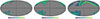 |
Fig. 2. Sky footprints of the QSO samples in Mollweide projection (HEALPix format with Nside = 64). Left to right: eBOSS DR14, eBOSS DR16, and DESI DR1. The maps show the number count per pixel for each catalogue. |
3. Method
3.1. Redshift dipole
The kinematic redshift dipole arises from the Doppler shift due to our peculiar motion relative to the cosmic rest frame. In an isotropic universe, the observed redshift distribution of distant sources should exhibit a dipolar anisotropy modulated by this motion. The dominant contribution to the observed redshift dipole Δ is our peculiar velocity v, expressed as β = v/c, where c is the speed of light. The theoretical relationship is given by Nadolny et al. (2021):
 (1)
(1)
where Δcd is the clustering dipole from large-scale structure, and 𝒪(β2) represents higher-order terms
Due to our motion, the observed frequency (ν) of light from a source in direction  is related to its rest-frame frequency νrest by
 (2)
(2)
Using c = λν and the definition of redshift z = (λobserve − λemit)/λemit, we derived the Lorentz boost relation between the observed redshift z′ (in the observer’s frame) and the intrinsic redshift z (in the CMB rest frame):
 (3)
(3)
The term z represents the expected redshift in an isotropic universe.
For high-redshift sources (z ≳ 1), such as the QSOs used here, the clustering dipole contribution Δcd is significantly suppressed compared to the kinematic term (Tiwari & Nusser 2016). Therefore, to first approximation, we assumed Δ ≈ −β when translating a measured dipole into a peculiar velocity.
3.2. Estimator
Following the tomographic methodology of da Silveira Ferreira & Marra (2024), we estimated the kinematic dipole by analysing the redshift distribution in fine bins. This approach mitigates the impact of large-scale clustering noise and allows us to probe potential redshift evolution of the signal.
We divided the QSO sample into narrow redshift bins of width Δz = 0.001. For each bin, we modelled the observed redshift z′i as a Doppler-shifted version of an intrinsic, isotropic redshift field. The goal is to determine the dipole vector Δ = (Δx, Δy, Δz) defined in the Cartesian coordinate system transformed from Galactic coordinates (x towards the Galactic centre, y in the direction of Galactic rotation, and z towards the North Galactic Pole), and a monopole offset m that best match this model. This is achieved by minimizing a per-bin χ2 statistic using a least-squares estimator. In practice, we employed the fit_dipole function from the HEALPix package (Gorski et al. 2005), which performs this fit on a spherical harmonic representation of the data within the bin.
The core of the estimator compares the observed redshifts with a simulated isotropic field. For a trial dipole Δ, we first computed the Lorentz boost factor  for each QSO i in direction
  . We then constructed a simulated intrinsic redshift for the bin,
  , by removing the estimated Doppler shift from all objects and computing the weighted mean:
 (4)
(4)
This  represents our best estimate of what the redshift would be in the CMB rest frame for that bin, given the current Δ. The N denotes the total number of objects. The total weights wi = wi, sys ⋅ wi, fail are derived from the LSS catalogues, where wi, sys represents the systematic weight and wi, fail the redshift failure weight. We emphasize that the weight definition is consistent for both the eBOSS and DESI catalogues used in this analysis. Next, we applied the boost to this intrinsic value to predict what we should observe if Δ were correct:
  . The χ2 for the bin measures the discrepancy between the actual observations z′i and these predictions z″i, bin:
![Mathematical equation: $$ \begin{aligned} \chi _{\rm bin}^2(\boldsymbol{\Delta }) = \frac{\sum _{i}^{N}w_{i}[1+z\prime _{i}-(1+z{\prime \prime }_{i,\mathrm{bin}})]^2}{\sum _{i}^{N}w_{i}}\cdot \end{aligned} $$](/articles/aa/full_html/2026/04/aa56955-25/aa56955-25-eq11.gif) (5)
(5)
The estimator iteratively adjusts Δ to minimize χbin2. The minimization process aims to fit a reference frame that is as stationary as possible relative to the CMB. This was achieved by removing our peculiar velocity. It should be noted that, since the peculiar velocity of the observed objects is unknown, we relied solely on the Earth’s peculiar velocity and the statistical characteristics of the material reference frame for the fit. As mentioned in Section 3.4, the distant material reference frame should remain relatively stationary with respect to the CMB as a whole.
3.3. Unbiased estimation
As established in Section 2 and Figure 3, significant systematic differences exist between the NGC and SGC. A joint fit to the combined data, assuming a single global monopole, would be biased because the mean redshift (the monopole) differs between hemispheres. To obtain an unbiased estimate of the dipole – which should be a global vector – we must account for these hemispheric offsets.
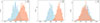 |
Fig. 3. Assessment of NGC and SGC systematic differences via bootstrap resampling. For each QSO sample (left: eBOSS DR14; centre: eBOSS DR16; right: DESI DR1), we repeatedly (1000 times) drew bootstrap resamples of 28 000 data points from each hemisphere’s dataset, computing the mean redshift for each resample. The distributions of these resampled means are plotted as histograms with a bin width of 0.000333. The y-axis represents the count of resamples whose mean redshift falls within the corresponding bin. All distributions are plotted relative to the average redshift of the total NGC dataset (vertical line at zero). The x-axis shows the redshift difference Δz (dimensionless) relative to the total NGC mean. The offset between the NGC (centred) and SGC distributions indicates a hemisphere-level systematic discrepancy. The amplitude of this offset (∼0.008 for eBOSS, ∼0.001 for DESI) is comparable to the expected kinematic dipole signal (β = v/c ∼ 10−3), necessitating separate hemispheric analysis (Section 3.3). |
The key to our unbiased estimation is to perform the dipole fit separately on the NGC and SGC datasets while enforcing consistency in the resulting dipole vector. If the two Galactic caps are analysed together, the dipole calculation would be adjusted relative to the combined monopole of both hemispheres, introducing systematic differences of the same order–or larger–than the expected dipole signal (cΔ ∼ 300 km/s). We therefore analysed the NGC and the SGC independently.
In practice, within each redshift bin, we minimized χbin, NGC2(Δ) and χbin, SGC2(Δ), allowing the fit in each hemisphere to account for its own redshift weighting. Crucially, we then required that the dipole vector Δ that minimizes the combined χtotal2 in Equation (6) be identical for both hemispheres. This approach effectively avoids the bias introduced by merging the data; it extracts a single, coherent kinematic dipole signal consistent across the full sky.
We implemented this by performing the minimization separately for the NGC and the SGC samples within each redshift bin. This yields two χ2 functions: χbin, NGC2(Δ) and χbin, SGC2(Δ), each already marginalized over their respective hemispheric monopoles. The total χ2 for the entire dataset is then the sum over all bins and both hemispheres:
![Mathematical equation: $$ \begin{aligned} \chi ^2_{\mathrm{total} }(\boldsymbol{\Delta }) = \sum \left[\chi ^2_{\mathrm{bin,NGC} }(\boldsymbol{\Delta }) + \chi ^2_{\mathrm{bin,SGC} }(\boldsymbol{\Delta })\right]. \end{aligned} $$](/articles/aa/full_html/2026/04/aa56955-25/aa56955-25-eq12.gif) (6)
(6)
Minimizing χtotal2(Δ) yields the dipole estimate Δ that best fits the data while being insensitive to the NGC-SGC mean redshift offset.
3.4. Fisher’s statistical method
To quantitatively assess the tension between our measured dipole and the prediction from the CMB kinematic dipole (ΔCMB), we needed a single statistical measure that combines the evidence from all three Cartesian components. Fisher’s combined probability test (Fisher 1925) provides a rigorous framework for this.
For each Cartesian component k ∈ x, y, z, we defined a null hypothesis H0(k): the measured dipole component Δk is consistent with the CMB-predicted value ΔCMB, k. We computed the corresponding p-value, Pk, which represents the probability of obtaining a value as extreme as or more extreme than our measurement Δk if H0(k) were true. Assuming Gaussian errors, Pk is derived from the two-tailed test statistic |Δk − ΔCMB, k|/σ, where  , since the CMB dipole is measured with high precision.
Following the CP and the work of Ellis & Baldwin (1984), the matter reference frame defined by distant objects is expected to be at rest relative to the CMB on large scales, meaning that an isotropic and homogeneous reference frame should not systematically bias any particular dipole component. Based on this, we assumed that the tests for the three orthogonal components are independent, Fisher’s method combines the p-values into a single test statistic:
 (7)
(7)
If all individual null hypotheses are true and the test statistics |Δk − ΔCMB, k| are independent, the test statistic X2 follows a χ2 distribution with 2 × 3 = 6 degrees of freedom.
The final combined p-value, Pcombined, was calculated as the survival function of the χ62 distribution at the observed X2. A very small Pcombined indicates a low probability that all three CMB dipole component predictions are simultaneously consistent with our measurements. This combined p-value was then converted into a significance level in units of Gaussian standard deviations (σ). This metric provides a comprehensive and conservative measure of the overall discrepancy between the large-scale structure dipole and the CMB dipole.
4. Discussion and conclusion
In this study, we presented a test of the CP by measuring the large-scale structure dipole anisotropy using QSO samples from eBOSS DR14 (0.4 < z < 2.8), DR16 (0.6 < z < 2.2), and DESI DR1 (0.8 < z < 3.0). Our analysis, employing the methodology of da Silveira Ferreira & Marra (2024), allows for a direct comparison of the kinematic dipole inferred from the distribution of QSOs with the canonical CMB dipole. The key results, summarized in Table 2 and Fig. 4, reveal a complex picture that warrants careful scientific discussion.
 |
Fig. 4. Empirical distribution plots of the DESI DR1 redshift dipole in its Cartesian components (m, cΔx, cΔy, cΔz). The red curve represents the dipole expected from the CMB dipole. The x-axis represents velocity (in kilometres per second), the y-axis represents distribution density, and the shaded regions denote the 1σ confidence intervals. Notably, the cΔy component shows small deviation from the CMB prediction, while the 1σ ranges of both cΔx and cΔz fully encompass the CMB dipole value. |
Three QSO catalogues dipole result, with 1σ range.
From the DESI DR1 data, we infer a bulk flow velocity of v = 443.8 ± 204.1 km/s towards (l, b) = (107.4° ±86.8° ,28.4° ±45.2° ). While the velocity magnitude is consistent with the CMB kinematic value of 370 km/s within 1.56σ, the best-fit direction shows a substantial offset from the CMB dipole (l = 264.02° ,b = 48.25° ). However, a component-by-component statistical assessment using Fisher’s method yields an overall tension of 3.45σ for DESI, primarily driven by a deviation in the Δy component. To interpret these seemingly contradictory signals – a consistent velocity magnitude but offset Δy direction and component level tension – we considered the evidence in a broader context.
Internal consistency and data evolution: The progression from the highly anomalous eBOSS DR14 result to the CMB-consistent eBOSS DR16 result underscores the critical impact of data quality. The DR14 discrepancy is likely attributable to its smaller sample size and higher redshift dispersion, limitations mitigated in DR16. This evolution cautions against over-interpreting significant tensions from any single data release, including the 3.45σ value from DESI DR1.
Methodological validation and external comparison: Our successful replication of the da Silveira Ferreira & Marra (2024) analysis on the eBOSS DR16 QSO sample yields a consistent result. We derive a bulk flow of v = 477.6 ± 224.4 km/s towards (l, b) = (261.4° ±117.3° , − 0.4° ±34.6° ), in agreement with the CMB kinematic dipole at a 2.1σ level (see Fig. A.1). This is in close agreement with their original finding of  km/s towards
  , which they reported as consistent with the CMB kinematic expectation at a 2σ level. This independent verification validates our analytical framework and, crucially, confirms that the methodology itself does not inherently produce high-tension results. The discrepancy, therefore, arises specifically with the DESI DR1 sample, suggesting sample-specific factors may be at play.
The nature of the 3.45σ tension in DESI: The significant Fisher combined tension for DESI warrants careful dissection. As Fig. 4 shows, it stems largely from the Δy component, whose associated unipolar amplitude differs from the expected value by nearly 300 km/s. This deviation may originate from the data itself, potentially challenging the CP. This pattern–a component-isolated deviation–is more indicative of residual systematic effects or unusual sample variance within DESI’s specific scan pattern and calibration, rather than a coherent, all-sky anisotropy expected from a genuine breakdown of isotropy.
The central question is whether the measured dipole reflects our motion relative to the Hubble flow (kinematic origin, supporting CP) or an intrinsic anisotropy (challenging CP). The amplitude of the DESI-inferred bulk flow is consistent with the kinematic expectation, which is a necessary condition for the kinematic interpretation. However, the offset in the best-fit direction, though not statistically significant given the large uncertainties, introduces ambiguity. Claims of a CP violation require not only high statistical significance but also robustness across multiple independent probes, elimination of plausible systematics, and a consistent directional signal across different redshift slices and tracers. Our DESI result, characterized by a component-level tension and a direction that is not robustly constrained, currently falls short of these stringent criteria.
In conclusion, our analysis employed the inferred bulk flow velocity–derived from the dipole–as the critical test. The amplitude of this velocity, at |v| = 443.8 ± 204.1 km/s, is consistent with the kinematic interpretation of the CMB dipole within 1.56σ. However, its direction (l, b) = (107.4° ±86.8° ,28.4° ±45.2° ) shows a notable offset from the CMB dipole, though with large uncertainties. The significant statistical tension (3.45σ) is primarily localized to the Δy component, which exhibits a large deviation. Crucially, the Δx and Δz components are in good agreement with expectations (see Fig. 4). This pattern–a coherent amplitude, a directionally ambiguous vector with two well-behaved components–suggests that the tension is more likely driven by residual systematics or sample variance in DESI DR1, rather than by cosmological anisotropy. Therefore, the current measurements do not provide compelling evidence against the CP. Future, larger datasets will be essential to reduce uncertainties and clarify the origin of the Δy anomaly.
Data availability
The eBOSS data are available at https://data.sdss.org/sas/dr16/eboss. The DESI data are available at https://data.desi.lbl.gov/public/dr1.
Acknowledgments
This work was supported by the National SKA Program of China (Grants Nos. 2022SKA0110200 and 2022SKA0110203). This work was also supported by Xiaofeng Yang’s ZHISHAN Distinguished Professor startup funding of Henan University.
References
- Abolfathi, B., Aguado, D. S., Aguilar, G., et al. 2018, ApJS, 235, 42 [NASA ADS] [CrossRef] [Google Scholar]
- Adame, A., Aguilar, J., Ahlen, S., et al. 2025, JCAP, 2025, 017 [Google Scholar]
- Aghanim, N., Akrami, Y., Arroja, F., et al. 2020, A&A, 641, A1 [NASA ADS] [CrossRef] [EDP Sciences] [Google Scholar]
- Bengaly, C. A. P., Bernui, A., Ferreira, I. S., & Alcaniz, J. S. 2016, MNRAS, 466, 2799 [Google Scholar]
- Blake, C., & Wall, J. 2002, Nature, 416, 150 [NASA ADS] [CrossRef] [Google Scholar]
- Böhme, L., Schwarz, D. J., Tiwari, P., et al. 2025, Phys. Rev. Lett., 135, 201001 [Google Scholar]
- Clowes, R. G., Harris, K. A., Raghunathan, S., et al. 2013, MNRAS, 429, 2910 [Google Scholar]
- da Silveira Ferreira, P., & Marra, V. 2024, JCAP, 2024, 077 [Google Scholar]
- Dam, L., Lewis, G. F., & Brewer, B. J. 2023, MNRAS, 525, 231 [NASA ADS] [CrossRef] [Google Scholar]
- DESI Collaboration (Abdul-Karim, M., et al.) 2025, ArXiv e-prints [arXiv:2503.14745] [Google Scholar]
- Ellis, G. F. R., & Baldwin, J. E. 1984, MNRAS, 206, 377 [NASA ADS] [CrossRef] [Google Scholar]
- Eriksen, H. K., Hansen, F. K., Banday, A. J., Gorski, K. M., & Lilje, P. B. 2004, ApJ, 605, 14 [NASA ADS] [CrossRef] [Google Scholar]
- Fisher, R. A. 1925, Statistical Methods for Research Workers (London: Oliver and Boyd) [Google Scholar]
- Franco, C., Avila, F., & Bernui, A. 2023, MNRAS, 527, 7400 [Google Scholar]
- Friday, T., Clowes, R. G., & Williger, G. M. 2022, MNRAS, 511, 4159 [Google Scholar]
- Gibelyou, C., & Huterer, D. 2012, MNRAS, 427, 1994 [NASA ADS] [CrossRef] [Google Scholar]
- Gorski, K. M., Hivon, E., Banday, A. J., et al. 2005, ApJ, 622, 759 [Google Scholar]
- Gupta, S., & Saini, T. D. 2010, MNRAS, 407, 651 [Google Scholar]
- Haslbauer, M., Banik, I., & Kroupa, P. 2020, MNRAS, 499, 2845 [Google Scholar]
- Hinshaw, G., Weiland, J. L., Hill, R. S., et al. 2009, ApJS, 180, 225 [Google Scholar]
- Keenan, R. C., Barger, A. J., & Cowie, L. L. 2013, ApJ, 775, 62 [Google Scholar]
- Lyke, B. W., Higley, A. N., McLane, J. N., et al. 2020, ApJS, 250, 8 [NASA ADS] [CrossRef] [Google Scholar]
- Nadolny, T., Durrer, R., Kunz, M., & Padmanabhan, H. 2021, JCAP, 2021, 009 [CrossRef] [Google Scholar]
- Oayda, O. T., Mittal, V., Lewis, G. F., & Murphy, T. 2024, ArXiv e-prints [arXiv:2406.01871] [Google Scholar]
- Park, C.-G., Hyun, H., Noh, H., & Hwang, J.-C. 2017, MNRAS, 469, 1924 [Google Scholar]
- Planck Collaboration XVI. 2016, A&A, 594, A16 [NASA ADS] [CrossRef] [EDP Sciences] [Google Scholar]
- Planck Collaboration VII. 2020, A&A, 641, A7 [NASA ADS] [CrossRef] [EDP Sciences] [Google Scholar]
- Ralston, J. P., & Jain, P. 2004, Int. J. Mod. Phys. D, 13, 1857 [Google Scholar]
- Rameez, M., Mohayaee, R., Sarkar, S., & Colin, J. 2018, MNRAS, 477, 1772 [Google Scholar]
- Ross, A. J., Bautista, J., Tojeiro, R., et al. 2020, MNRAS, 498, 2354 [NASA ADS] [CrossRef] [Google Scholar]
- Rubart, M., & Schwarz, D. J. 2013, A&A, 555, A117 [NASA ADS] [CrossRef] [EDP Sciences] [Google Scholar]
- Rubart, M., Bacon, D., & Schwarz, D. J. 2014, A&A, 565, A111 [Google Scholar]
- Sarkar, S., Pandey, B., & Khatri, R. 2018, MNRAS, 483, 2453 [Google Scholar]
- Secrest, N. J., Hausegger, S. V., Rameez, M., et al. 2021, ApJ, 908, L51 [Google Scholar]
- Secrest, N. J., von Hausegger, S., Rameez, M., Mohayaee, R., & Sarkar, S. 2022, ApJ, 937, L31 [NASA ADS] [CrossRef] [Google Scholar]
- Singal, A. K. 2011, ApJ, 742, L23 [NASA ADS] [CrossRef] [Google Scholar]
- Singal, A. K. 2022, MNRAS, 515, 5969 [Google Scholar]
- Sorrenti, F., Durrer, R., & Kunz, M. 2023, ArXiv e-prints [arXiv:2212.10328] [Google Scholar]
- Tiwari, P., & Nusser, A. 2016, JCAP, 2016, 062 [Google Scholar]
- Wu, K. K. S., Lahav, O., & Rees, M. J. 1999, Nature, 397, 225 [Google Scholar]
- Yang, X., Wang, F. Y., & Chu, Z. 2013, MNRAS, 437, 1840 [Google Scholar]
Appendix A: Methodological validation and additional analyses
This appendix provides supporting details for the dipole analysis presented in the main text, focusing on methodological consistency and the exploration of potential systematics.
As a primary validation step of our entire analysis pipeline—including data processing, dipole estimation, and uncertainty quantification—we applied it to the eBOSS DR16 QSO sample. This is the same dataset used in the benchmark study of (da Silveira Ferreira & Marra 2024).
We followed the identical procedure outlined in Section 3 of the main text. The sample selection, coordinate transformations, and likelihood analysis for the dipole components were performed without modification.
The resulting probability distributions for the monopole and the three Cartesian dipole components are shown in Fig. A.1 in the main text. The key outcome is that the expected value from the CMB kinematic dipole (red line) falls entirely within the 1σ posterior credible interval for every single component.
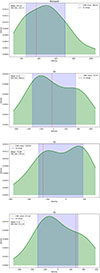 |
Fig. A.1. Empirical distribution plots of the eBOSS DR16 redshift dipole in its Cartesian components (m, cΔx, cΔy, cΔz). The red curve represents the dipole expected from the CMB dipole. The x-axis represents velocity (in km/s), the y-axis represents distribution density, and the shaded regions denote the 1σ confidence intervals. Notably, all components fully encompass the CMB dipole value at the 1σ ranges. |
This successful replication serves two crucial purposes: 1. Methodological Robustness: It confirms that our implementation of the (da Silveira Ferreira & Marra 2024) method is correct and yields consistent results on the same data. 2. Baseline Establishment: It provides a clear benchmark for a “consistent” result within the ΛCDM framework. The contrast between this clean consistency (eBOSS DR16) and the component-level tension found in DESI DR1 (Fig. 4) sharpens the discussion on the origin of the latter.
All Tables
All Figures
|
Fig. 1. Redshift distributions of the QSO catalogues. Left to right: eBOSS DR14 (orange), eBOSS DR16 (green), and DESI DR1 (blue). The DR14 distribution is broad (0.4 < z < 8) but sparse at the extremes; we use the well-populated range 0.4 < z < 2.8. The DESI DR1 distribution spans 0.8 < z < 3.5; we use 0.8 < z < 3.0 to avoid edge effects. All histograms use a bin width of Δz = 0.001. Note that the y-axis scales differ between panels. The primary overlap region for the eBOSS samples is 0.8 < z < 2.2, while DESI significantly overlaps in the range 0.8 < z < 2.3. |
| In the text | |
|
Fig. 2. Sky footprints of the QSO samples in Mollweide projection (HEALPix format with Nside = 64). Left to right: eBOSS DR14, eBOSS DR16, and DESI DR1. The maps show the number count per pixel for each catalogue. |
| In the text | |
|
Fig. 3. Assessment of NGC and SGC systematic differences via bootstrap resampling. For each QSO sample (left: eBOSS DR14; centre: eBOSS DR16; right: DESI DR1), we repeatedly (1000 times) drew bootstrap resamples of 28 000 data points from each hemisphere’s dataset, computing the mean redshift for each resample. The distributions of these resampled means are plotted as histograms with a bin width of 0.000333. The y-axis represents the count of resamples whose mean redshift falls within the corresponding bin. All distributions are plotted relative to the average redshift of the total NGC dataset (vertical line at zero). The x-axis shows the redshift difference Δz (dimensionless) relative to the total NGC mean. The offset between the NGC (centred) and SGC distributions indicates a hemisphere-level systematic discrepancy. The amplitude of this offset (∼0.008 for eBOSS, ∼0.001 for DESI) is comparable to the expected kinematic dipole signal (β = v/c ∼ 10−3), necessitating separate hemispheric analysis (Section 3.3). |
| In the text | |
|
Fig. 4. Empirical distribution plots of the DESI DR1 redshift dipole in its Cartesian components (m, cΔx, cΔy, cΔz). The red curve represents the dipole expected from the CMB dipole. The x-axis represents velocity (in kilometres per second), the y-axis represents distribution density, and the shaded regions denote the 1σ confidence intervals. Notably, the cΔy component shows small deviation from the CMB prediction, while the 1σ ranges of both cΔx and cΔz fully encompass the CMB dipole value. |
| In the text | |
|
Fig. A.1. Empirical distribution plots of the eBOSS DR16 redshift dipole in its Cartesian components (m, cΔx, cΔy, cΔz). The red curve represents the dipole expected from the CMB dipole. The x-axis represents velocity (in km/s), the y-axis represents distribution density, and the shaded regions denote the 1σ confidence intervals. Notably, all components fully encompass the CMB dipole value at the 1σ ranges. |
| In the text | |
Current usage metrics show cumulative count of Article Views (full-text article views including HTML views, PDF and ePub downloads, according to the available data) and Abstracts Views on Vision4Press platform.
Data correspond to usage on the plateform after 2015. The current usage metrics is available 48-96 hours after online publication and is updated daily on week days.
Initial download of the metrics may take a while.