| Issue |
A&A
Volume 700, August 2025
|
|
|---|---|---|
| Article Number | L1 | |
| Number of page(s) | 7 | |
| Section | Letters to the Editor | |
| DOI | https://doi.org/10.1051/0004-6361/202555720 | |
| Published online | 25 July 2025 | |
Letter to the Editor
Phase reddening of Phobos and Deimos from TGO/CaSSIS observations
1
INAF Astronomical Observatory of Padova, Vicolo dell’Osservatorio 5, 35122 Padova, Italy
2
CISAS, Università degli Studi di Padova, Padova, Italy
3
Physikalisches Institut, Sidlerstr. 5, University of Bern, CH-3012 Bern, Switzerland
4
School of Physical Sciences, The Open University, Walton Hall, Milton Keynes, UK
5
Brown University, Department of Earth, Environmental and Planetary Sciences, 180 Thayer St, Providence, RI 02912, USA
⋆ Corresponding author: This email address is being protected from spambots. You need JavaScript enabled to view it.
Received:
29
May
2025
Accepted:
26
June
2025
Abstract
Aims. We study the phase-reddening effect (i.e. the increase in spectral slope with phase angle) of Phobos and Deimos, with the aim of characterising the origin and physical properties of the two Martian moon surfaces and spectral units.
Methods. We analysed Phobos and Deimos four-filter observations at visible to near-infrared wavelengths acquired by the Colour and Surface Stereo Imaging System (CaSSIS) on board ESA’s ExoMars Trace Gas Orbiter (TGO) over a wide range of phase angles. From these observations, we derived the spatial distribution of the phase reddening and spectral slope over the sub-Mars hemispheres of Phobos and Deimos.
Results. We present the first spatially resolved map of the Phobos phase reddening and the first estimate of the Deimos global phase reddening in the visible to near-infrared wavelengths.
Conclusions. Our results suggest that (i) the surface of Phobos is characterised by variable phase reddening, (ii) the phase reddening of Deimos is similar to that of the redder units on Phobos, (iii) the amount of phase reddening is linked to regolith maturity and can be explained by space-weathering, (iv) the Phobos Blue unit post-dates the Stickney impact and may have an exogenous origin, and (v) the physical properties of the regolith on Phobos and Deimos are different from those of Martian regolith.
Key words: planets and satellites: composition / planets and satellites: formation / planets and satellites: surfaces / planets and satellites: terrestrial planets / planets and satellites: individual: Phobos / planets and satellites: individual: Deimos
© The Authors 2025
 Open Access article, published by EDP Sciences, under the terms of the Creative Commons Attribution License (https://creativecommons.org/licenses/by/4.0), which permits unrestricted use, distribution, and reproduction in any medium, provided the original work is properly cited.
This article is published in open access under the Subscribe to Open model. This email address is being protected from spambots. You need JavaScript enabled to view it. to support open access publication.
1. Introduction
Phobos and Deimos are the two moons of Mars. The diameter of the first moon is 22 km, and it orbits the planet at a distance of 9377 km, and the diameter of the second moon is 12 km, and it orbits 23 460 km from Mars. Despite more than 45 years of dedicated or serendipitous multi-instrument observations (Witasse et al. 2014; Pascu et al. 2014), the origin of the moons is still an open and largely debated conundrum. Current hypotheses envision a capture of primitive asteroids or comets (Pajola et al. 2012; Hansen 2018; Fornasier et al. 2024; Kegerreis et al. 2025) or in situ formation by either co-accretion with Mars or re-accretion from impact-generated debris (Rosenblatt 2011; Craddock 2011; Hyodo et al. 2017). The first scenario is supported by the similarity in the spectra of the moons and D-type (primitive carbonaceous) asteroids (Murchie & Erard 1996; Rivkin et al. 2002; Pajola et al. 2013) and with the photometric properties of 67P (Fornasier et al. 2024). The latter scenario explains the near-circular equatorial orbits of the moons (Craddock 2011; Rosenblatt 2011), but is inconsistent with the spectroscopy (Nakamura et al. 2021; Takir et al. 2022). A key goal of the upcoming JAXA Martian Moons eXploration (MMX) sample-return mission is an answer to this question (Kuramoto et al. 2022).
Spectroscopic and imaging data revealed that the Phobos surface is heterogeneous and exhibits at least two spectral units: a predominantly red unit distributed throughout Phobos, and a less-red (blue) unit that is located on the leading sub-Mars hemisphere near the impact crater Stickney (Murchie & Erard 1996; Fraeman et al. 2012, 2014; Pajola et al. 2018). The latter was initially considered as the fresh ejecta deposit excavated from the Phobos interior by the Stickney impact, but an exogenic origin from remnants of the impactor in a low-velocity impact cannot be ruled out either (Basilevsky et al. 2014; Takir et al. 2017). An intermediate transitional unit has also been identified from OMEGA hyperspectral data (Pajola et al. 2025). Deimos, in contrast, appears to be more spectrally uniform and similar to the Red unit of Phobos (Fraeman et al. 2014).
Photometric analyses of the Martian moons were largely focused on Phobos (Avanesov et al. 1991; Simonelli et al. 1998; Cantor et al. 1999; Pajola et al. 2012; Fraeman et al. 2012; Fornasier et al. 2024), while Deimos is less studied (Klaasen et al. 1979; Pang et al. 1983) and defined photometric models for Phobos and Deimos that allowed characterising their albedo, phase function, and spectral slope across their surface units. One photometric property of particular interest is phase reddening, that is, the increase in spectral slope with phase angle that is attributed to multiple scattering, surface roughness at the sub-micron level, and space-weathering (Sanchez et al. 2012; Schröder et al. 2014; Sato et al. 2014). Investigating this helps us to constrain the physical properties of the Martian moon surfaces in terms of the particle size and roughness.
The Colour and Surface Stereo Imaging System (CaSSIS) is a multi-filter stereo camera on board the ExoMars Trace Gas Orbiter (TGO) satellite (Thomas et al. 2017). It provides images of the Martian surface at 4.6 m/px in four filters centred at (effective wavelength ± equivalent bandwidth) 499.9 ± 118.0 nm (BLU), 675.0 ± 229.4 nm (PAN), 836.2 ± 94.3 nm (RED), and 936.7 ± 113.7 nm (near-IR; NIR) with a radiometric accuracy of 2.8% (Thomas et al. 2022). After multiple years entirely focusing on the Martian surface, CaSSIS has recently had the possibility of targeting Phobos and Deimos at different phase angles and spatial resolutions of ≈60–120 m/px and ≈ 200–300 m/px, respectively. We present the analysis of the CaSSIS observations of the Martian moons, the first characterisation of the spatial distribution of the phase reddening on Phobos, and its variability among specific geological units. In addition, we provide the first estimate of the global phase reddening on Deimos by performing a comparative analysis with Phobos.
2. Methods
We analysed 35 CaSSIS observations of Phobos and 4 observations of Deimos that spanned phase angles of 0.8 − 83.0° and 14.2 − 49.5°, respectively. The observation details are given in Tables A.1 and A.2. CaSSIS observes in push-frame mode and acquires all four filters simultaneously (Thomas et al. 2017). Therefore, multiple acquisition with Phobos (or Deimos) centred on each filter FoV are needed for a multi-band mosaic. This is typically accomplished in less than two minutes and implies that the illumination and observation conditions between each filter are the same. For each observation, we aligned all filters to the PAN using the software elastix (Klein et al. 2010). We obtained a four-band cube. Through SPICE (Acton 1996; Acton et al. 2018) we computed the local angles of incidence, phase, emission, and the latitude and longitude for each cube pixel, as in Stooke & Pajola (2019), for example. We used the shape models of Ernst et al. (2023) of Phobos and Deimos with a ground sampling distance of 18 m and 20 m, respectively Ernst et al. (2023). An example of a Phobos and Deimos RGB colour composite from the CaSSIS NIR-PAN-BLU bands and local incidence (i) and emission (e) angles is shown in Fig. 1. Since Deimos has very little spectral variability and a relatively low number of images, we opted for a very simple and straightforward approach and computed the average NIR/BLU filter ratio for each observation as a proxy for spectral slope. This ratio is not affected by shading, and therefore, no topographic correction (i.e. as in Pajola et al. 2012; Munaretto et al. 2021; Pajola et al. 2025) was required. It offers the largest wavelength baseline (499.9 nm to 936.7 nm) for evaluating the spectral slope with CaSSIS. Our formulation differs slightly from the usual spectral slope formulation, that is, SS  , with λ1 and λ2 being two wavelengths, and Rλ1, Rλ2 the corresponding reflectances (Fornasier et al. 2015, 2020). The latter relies on different wavelengths, however, which makes comparisons challenging. Our plain NIR/BLU can easily be converted into the usual notation with the formula (NIR/BLU-1)/(936.7–499.9), and it has been used for CaSSIS-based phase-reddening studies (Valantinas et al. 2025). For the above reasons, we adopted the most straightforward approach and considered the NIR/BLU ratio as a proxy for the spectral slope. We collected NIR/BLU versus phase angle for all the four Deimos observations and took the error in the NIR/BLU given by each filter 1σ standard deviation into account. We fitted this dataset with a linear model whose parameters allowed us to estimate the global spectral slope of the Deimos zero-phase angle (model intercept) and the global phase reddening coefficient of Deimos (model linear term). Many more overlapping observations are instead available for Phobos, and we therefore also analysed the spatial distribution of the phase reddening and spectral slopes. This required a different approach. We defined a latitude-longitude grid with a resolution of 1° ×1°. For each grid point, we collected data (i.e. NIR/BLU and phase angle) from all the observations that covered this location, and we fitted this dataset using a bootstrap approach (Bradley & Tibshirani 1993) to obtain maps of the phase reddening and zero-phase spectral slope. The fitting details are given in Appendix B). To analyse specific locations of Phobos with higher accuracy, we defined regions of interest (ROIs; Fig. 2) and repeated the fit with all data from these ROIs. The ROIs have different stages of regolith maturity. ROIs R1 to R3 are picked on the Red Unit as representatives of the oldest and most mature regolith of Phobos. LIMTOC was selected within the relatively fresher Limtoc crater (Fig. C.1d). B2 samples mature Blue unit material, and cr was selected on a crater younger than B2 that exposes material from the underlying Red unit (Fig. C.1b). B1 (Figs. C.1a and 2) is representative of less space weathered Blue unit material deposited by fresh crater ejecta (blue circles in Fig. C.1a). While it is unclear in principle whether B2 post or pre-dates LIMTOC, the cr and B1 ROI are most likely fresher. The latter sample craters with well-visible and preserved ejecta (arrows in Figs. C.1b,c), which is a typical fingerprint of Phobos fresh craters that are instead absent inside Limtoc and B2.
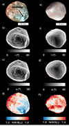 |
Fig. 1. CaSSIS NIR-PAN-BLU observations of Phobos (left) and Deimos (right). a and e: Colour composites. b and f: Local incidence. c and g: Emission angle maps. d and h: NIR/BLU maps. |
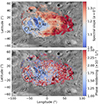 |
Fig. 2. Zero-phase angle NIR/BLU spectral slope (a) and phase-reddening spatial distribution (b) overlaid on the Phobos Viking global mosaic (Simonelli et al. 1993). The black polygons indicate the name and position of the ROIs. |
3. Results
We obtained the zero-phase spectral slope map (Fig. 2a), as well as the first spatially resolved phase-reddening map (Fig. 2b) at a resolution of 1° ×1° of the portion of the Phobos sub-Mars (i.e., near side) hemisphere observed by CaSSIS. These maps visually represent the variation in the phase reddening and spectral slope across the Phobos surface. In particular, they confirm that the variability in the spectral slope of Phobos is dominated by the Blue unit (lower spectral slopes), which transitions to the Red unit (higher spectral slope). Interestingly, the phase reddening is not uniform on the surface, but is lower in regions that broadly correspond to the Blue unit. We plot in Fig. 3 the fitted phase reddening and spectral slope for different Phobos units and Deimos. The model parameters and associated uncertainties are reported in Table 1. In particular, the Phobos Red unit ROIs (R1, R2, and R3) have the highest phase reddening and it is consistent with that of Deimos, and they have the highest spectral slope. The Limtoc crater ROI has a relatively lower phase reddening, followed by the B2 ROI (representative of unaltered Blue unit material). The cr ROI has a smaller phase reddening than the B2 unit, and finally, the B1 unit has the lowest phase-reddening coefficient. The Red unit ROIs have comparable and higher spectral slopes. Deimos has slightly lower spectral slopes, followed by the cr ROI. The Limtoc and the Blue units have the lowest spectral slope, as expected (i.e. Fornasier et al. 2024).
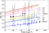 |
Fig. 3. NIR/BLU vs. phase-angle data for the Phobos ROIs and Deimos. The error bars are the 1σ standard deviations. The solid line shows the best-fit linear phase-reddening models, whose parameters are reported in Table 1. The vertical dashed lines indicate the range of the phase angles we used for the fits. The ROIs are defined in Fig. 2 and are described in Sect. 2. |
Average ROI phase-reddening coefficients and zero-phase NIR/BLU spectral slopes.
4. Discussion
The Red and Blue Phobos units are expected to originate from differences in the compositional and/or physical surface properties (Rosenblatt 2011; Ballouz et al. 2019). Phase reddening is sensitive to the microphysical properties of regolith, such as the surface roughness at the sub-micron level, and it has been correlated to the degree of space-weathering (Sanchez et al. 2012). In particular, space-weathered olivines, which are a good analogue for Phobos Xu et al. (2023), are characterised by the presence of sub-micron size nanophase iron (np-Fe0) particles. The roughness added by these space-weathering products may therefore induce a phase reddening of the surface. This is consistent with the phase-reddening map in Fig. 2b and with the ROI analysis summarised in Table 1, which show an increasing phase-reddening effect with regolith maturity. In particular, the older and most space-weathered units, represented by the Red unit on Deimos and Phobos (R1–R3). have the highest phase reddening (see Table 1). This gradually decreases with the transition to fresher units, that is, Limtoc and B2. The youngest and less space-weathered units B1 and cr have the weakest phase reddening. In this context, the phase reddening of the unaltered Blue unit ROI (B2) is intermediate between that of Limtoc and the cr ROI crater, which suggests that its emplacement occurred in between the two. This rules out its origin as material from Deimos and/or from Stickney ejecta. In these cases, it would be similarly space-weathered and present a phase reddening higher than Limtoc. Our results instead favour an emplacement of the Blue unit from exogenous material (Basilevsky et al. 2014; Takir et al. 2017) that occurred after the Limtoc and before the cr impacts.
The spatially resolved maps in Fig. 2 and the ROI analysis in Table 1 also suggest a possible trend between phase reddening and spectral slope. Our dataset does not allow us to separate the effects of phase reddening and compositional differences on the spectral slope, however. Any potential correlation between the spectral slope and the phase reddening should therefore be assessed through a compositional analysis.
Our results can also be compared with the phase-reddening analyses of Martian dust, which exhibits an arch-like curve that peaks at 40° phase (Valantinas et al. 2025) and is attributed to particle size. In contrast, we observe a monotonic reddening up to 60°. This suggests that the particle properties and possibly composition of the Martian dust or regolith are very different to those of Phobos and Deimos, and this agrees with compositional studies (Fraeman et al. 2012, 2014).
5. Conclusions
We presented a dataset of 35 observation of Phobos and 4 observations of Deimos acquired by TGO/CaSSIS. We summarise our main results and findings below.
-
We presented the first spatially resolved phase-reddening map of the sub-Mars hemisphere of Phobos at equatorial to medium latitudes. We identified a broad region that includes the Blue unit that is characterised by lower phase reddening surrounded by a higher phase-reddening surface.
-
We provided the first estimate of the Deimos phase reddening, which is comparable to that of the Phobos Red unit.
-
We found that the Phobos phase reddening increases with surface age and regolith maturity. This suggests that it originates from a sub-micron roughness that is added by space-weathering-sourced npFe0 particles that occurs at the moon.
-
We excluded an ejecta origin from Deimos or Stickney for the Blue unit. Instead, an exogenous nature is consistent with our results.
-
We found that the properties of the regolith on Phobos and Deimos are very different to those of Mars. This agrees with compositional studies.
The spatially resolved spectral slope and phase-reddening maps we presented will be useful in supporting the scientific activities of the future MMX mission and in selecting the best or freshest sampling sites on Phobos.
Acknowledgments
We gratefully acknowledge Dr. Driss Takir and Dr. Emmanuel Lellouch for providing insights that improved the paper. CaSSIS is a project of the University of Bern and funded through the Swiss Space Office via ESA’s PRODEX programme. The instrument hardware development was also supported by the Italian Space Agency (ASI) (ASI-INAF agreement no. 2020-17-HH.0), INAF/Astronomical Observatory of Padova, and the Space Research Center (CBK) in Warsaw. Support from SGF (Budapest), the University of Arizona (Lunar and Planetary Lab.) and NASA are also gratefully acknowledged. Operations support from the UK Space Agency under grant ST/R003025/1 is also acknowledged. We gratefully acknowledge support from the Italian Space Agency (ASI) with ASI-INAF agreements n. 2022-8-HH.0 and n. 2024-40-HH.0.
References
- Acton, C. H. 1996, Planet. Space Sci., 44, 65 [Google Scholar]
- Acton, C., Bachman, N., Semenov, B., & Wright, E. 2018, Planet. Space Sci., 150, 9 [Google Scholar]
- Avanesov, G., Zhukov, B., Ziman, Y., et al. 1991, Planet. Space Sci., 39, 281 [NASA ADS] [CrossRef] [Google Scholar]
- Ballouz, R.-L., Baresi, N., Crites, S. T., Kawakatsu, Y., & Fujimoto, M. 2019, Nat. Geosci., 12, 229 [CrossRef] [Google Scholar]
- Basilevsky, A. T., Lorenz, C. A., Shingareva, T. V., et al. 2014, Planet. Space Sci., 102, 95 [CrossRef] [Google Scholar]
- Bradley, E., & Tibshirani, R. J. 1993, An Introduction to the Bootstrap (New York: Chapman and Hall/CRC), Chapman Hall/CRC Monogr. Stat. Appl. Probab. [Google Scholar]
- Cantor, B. A., Wolff, M. J., Thomas, P. C., James, P. B., & Jensen, G. 1999, Icarus, 142, 414 [NASA ADS] [CrossRef] [Google Scholar]
- Craddock, R. A. 2011, Icarus, 211, 1150 [NASA ADS] [CrossRef] [Google Scholar]
- Ernst, C. M., Daly, R. T., Gaskell, R. W., et al. 2023, Earth Planets Space, 75, 103 [NASA ADS] [CrossRef] [Google Scholar]
- Fornasier, S., Hasselmann, P. H., Bartholucci, D., et al. 2015, A&A, 583, A30 [NASA ADS] [CrossRef] [EDP Sciences] [Google Scholar]
- Fornasier, S., Hasselmann, P. H., Deshapriya, J. D. P., et al. 2020, A&A, 644, A142 [NASA ADS] [CrossRef] [EDP Sciences] [Google Scholar]
- Fornasier, S., Wargnier, A., Hasselmann, P. H., et al. 2024, A&A, 686, A203 [NASA ADS] [CrossRef] [EDP Sciences] [Google Scholar]
- Fraeman, A. A., Murchie, S. L., Arvidson, R. E., et al. 2012, J. Geophys. Res., 117, E00J15 [Google Scholar]
- Fraeman, A. A., Murchie, S. L., Rivkin, A. S., et al. 2014, Icarus, 229, 196 [NASA ADS] [CrossRef] [Google Scholar]
- Hansen, B. M. S. 2018, MNRAS, 475, 2452 [CrossRef] [Google Scholar]
- Hyodo, R., Genda, H., Charnoz, S., & Rosenblatt, P. 2017, ApJ, 845, 125 [NASA ADS] [CrossRef] [Google Scholar]
- Kegerreis, J. A., Lissauer, J. J., Eke, V. R., Sandnes, T. D., & Elphic, R. C. 2025, Icarus, 425, 116337 [NASA ADS] [CrossRef] [Google Scholar]
- Klaasen, K. P., Duxbury, T. C., & Veverka, J. 1979, J. Geophys. Res., 84, 8478 [Google Scholar]
- Klein, S., Staring, M., Murphy, K., Viergever, M. A., & Pluim, J. P. W. 2010, IEEE Trans. Med. Imaging, 29, 196 [Google Scholar]
- Kuramoto, K., Kawakatsu, Y., Fujimoto, M., et al. 2022, Earth Planets Space, 74, 12 [NASA ADS] [CrossRef] [Google Scholar]
- McEwen, A. S., Eliason, E. M., Bergstrom, J. W., et al. 2007, J. Geophys. Res., 112, E05S02 [Google Scholar]
- Munaretto, G., Pajola, M., Lucchetti, A., et al. 2021, Planet. Space Sci., 200, 105198 [Google Scholar]
- Murchie, S., & Erard, S. 1996, Icarus, 123, 63 [CrossRef] [Google Scholar]
- Nakamura, T., Ikeda, H., Kouyama, T., et al. 2021, Earth Planets Space, 73, 227 [NASA ADS] [CrossRef] [Google Scholar]
- Pajola, M., Lazzarin, M., Bertini, I., et al. 2012, MNRAS, 427, 3230 [NASA ADS] [CrossRef] [Google Scholar]
- Pajola, M., Lazzarin, M., Dalle Ore, C. M., et al. 2013, ApJ, 777, 127 [NASA ADS] [CrossRef] [Google Scholar]
- Pajola, M., Roush, T., Dalle Ore, C., Marzo, G. A., & Simioni, E. 2018, Planet. Space Sci., 154, 63 [NASA ADS] [CrossRef] [Google Scholar]
- Pajola, M., Beccarelli, J., Munaretto, G., et al. 2025, A&A, 679, A56 [Google Scholar]
- Pang, K. D., Rhoads, J. W., Hanover, G. A., Lumme, K., & Bowell, E. 1983, J. Geophys. Res., 88, 2475 [NASA ADS] [CrossRef] [Google Scholar]
- Pascu, D., Erard, S., Thuillot, W., & Lainey, V. 2014, Planet. Space Sci., 102, 2 [Google Scholar]
- Rivkin, A. S., Brown, R. H., Trilling, D. E., Bell, J. F., & Plassmann, J. H. 2002, Icarus, 156, 64 [NASA ADS] [CrossRef] [Google Scholar]
- Rosenblatt, P. 2011, A&ARv, 19, 44 [CrossRef] [Google Scholar]
- Sanchez, J. A., Reddy, V., Nathues, A., & Moskovitz, N. 2012, Icarus, 220, 36 [CrossRef] [Google Scholar]
- Sato, H., Robinson, M. S., Hapke, B. W., Denevi, B. W., & Boyd, A. K. 2014, J. Geophys. Res., 119, 1775 [Google Scholar]
- Schröder, S. E., Grynko, Y., Pommerol, A., et al. 2014, Icarus, 239, 201 [Google Scholar]
- Simonelli, D. P., Thomas, P. C., Carcich, B. T., & Veverka, J. 1993, Icarus, 103, 49 [NASA ADS] [CrossRef] [Google Scholar]
- Simonelli, D. P., Wisz, M., Switala, A., et al. 1998, Icarus, 131, 52 [NASA ADS] [CrossRef] [Google Scholar]
- Stooke, P., & Pajola, M. 2019, Mapping Irregular Bodies, ed. H. Hargitai (Cham: Springer International Publishing), 191 [Google Scholar]
- Takir, D., Reddy, V., Sanchez, J. A., Shepard, M. K., & Emery, J. P. 2017, AJ, 153, 31 [Google Scholar]
- Takir, D., Matsuoka, M., Waiters, A., Kaluna, H., & Usui, T. 2022, Icarus, 371, 114691 [NASA ADS] [CrossRef] [Google Scholar]
- Thomas, N., Cremonese, G., Ziethe, R., et al. 2017, Space Sci. Rev., 212, 1897 [NASA ADS] [CrossRef] [Google Scholar]
- Thomas, N., Pommerol, A., Almeida, M., et al. 2022, Planet. Space Sci., 211, 105394 [NASA ADS] [CrossRef] [Google Scholar]
- Valantinas, A., Mustard, J. F., Chevrier, V., et al. 2025, Nat. Commun., 16, 1712 [Google Scholar]
- Witasse, O., Duxbury, T., Chicarro, A., et al. 2014, Planet. Space Sci., 102, 18 [Google Scholar]
- Xu, J., Mo, B., Wu, Y., et al. 2023, A&A, 672, A115 [NASA ADS] [CrossRef] [EDP Sciences] [Google Scholar]
Appendix A: Summary of Phobos and Deimos observations
We report in Tables A.1 and A.2 details of the CaSSIS observations of Phobos and Deimos used in this study. We plot in Fig. A.1 on a 1° ×1° latitude longitude grid the spatial distribution of the phase angle coverage (Figs. A.1a-c), as well as the number of data points (Fig. A.1d) and the accuracy of the phase-reddening and zero-phase spectral slope fits (Fig. A.1b) described in Appendix B.
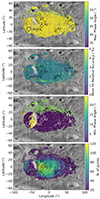 |
Fig. A.1. Maximum phase angle (a), mean fit relative accuracy (b), minimum phase angle (c), and number of points (d) for each grid point. |
CaSSIS Phobos observation details.
CaSSIS Deimos observation details.
Appendix B: Bootstrap fitting approach
We fitted the NIR/BLU vs phase angle data within each 1° ×1° grid point and within the selected ROIs with a linear model, i.e., y = mx + q. y represent NIR/BLU and x the phase angle (that we refer to with α). The model parameters are the linear slope m which represent the phase reddening coefficient and the intercept q that corresponds to the zero phase NIR/BLU spectral slope. In doing so, we filtered our dataset to phase angles < 60°. this criterion ensures that all locations have the same maximum phase angle, thereby avoiding possible correlations of the model parameters with maximum phase angle. An example is shown in fig. 3) and it is represented by the non-linear nature of phase reddening after ≈60°. This is the case for the B1, B2, LIMTOC and cr ROIs highlighting how regions with high phase angles observations could be sensitive to exponential phase reddening and their parameters could be biased accordingly. Potential biases could also come from the spatially variable number of data points in our dataset (Fig. A.1d) and their uneven phase angle coverage. In particular, Fig. 3 and Table A.1 highlight how phase angles between 40° and 80° are more densely sampled. To achieve uniform phase angle (α) sampling, we implement an inverse-probability resampling method. Given a set of data points  , coming from e.g., a ROI or a 1° ×1° grid point, we partition the phase angle range into N 1° non-empty bins. Let nj denote the number of data points falling into the j-th bin, with j = 1, 2, …, N. The original (non-uniform) sampling probability for each bin is then given by
 (B.1)
(B.1)
To correct for non-uniformity, we define the desired uniform sampling probability as
 (B.2)
(B.2)
The adjusted sampling weight for each bin, wj, is computed as the ratio
 (B.3)
(B.3)
Points within each bin inherit this bin-specific weight wj. The resulting sampling probability for the i-th data point, located in the j-th phase bin, is expressed as
 (B.4)
(B.4)
This method artificially increases the likelihood of sampling points from less populated bins while decreasing it in densely populated bins, thereby ensuring that if we extract a sample of points they will have a uniform phase distribution. We applied the bootstrap approach (Bradley & Tibshirani 1993) by repeatedly (1000 times) sampling 20 (the minimum from Fig. A.1d) data-points from e.g., a ROI or a 1° ×1° grid point and fitting them with a linear model. For each iteration, we obtained a set of model parameters. The final best-fitting parameters and their errors were estimated by calculating the average and standard deviation of the parameters collected from all the 1000 bootstrap iterations. This procedure was repeated for each grid point and for all the ROIs in Fig. 2.
Appendix C: Phobos imaged by HiRISE
Phobos was imaged by the High Resolution Imaging Science Experiment (HiRISE; McEwen et al. 2007) at 6.5 m/px on 23 March 2008. An RGB colour composite of the observation is shown in Fig. C.1, adapted from (Basilevsky et al. 2014). The original image is freely available at the HiRISE website1.
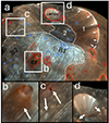 |
Fig. C.1. (a) RGB colour composite of Phobos from HiRISE image PSP_007769_9010, adapted from Basilevsky et al. (2014). Black labels indicate the approximate positions of the B1, B2, cr, and LIMTOC ROIs. Red and blue drawings indicate craters excavating Red and Blue unit materials, respectively. White lines indicate the approximate extent of the Blue unit and of Stickney floor (Basilevsky et al. 2014). Insets show close-ups of the cr ROI crater (b), visible ejecta of fresh craters (c), and the Limtoc crater and part of Stickney floor (d). Arrows indicate fresh crater ejecta. |
All Tables
Average ROI phase-reddening coefficients and zero-phase NIR/BLU spectral slopes.
All Figures
|
Fig. 1. CaSSIS NIR-PAN-BLU observations of Phobos (left) and Deimos (right). a and e: Colour composites. b and f: Local incidence. c and g: Emission angle maps. d and h: NIR/BLU maps. |
| In the text | |
|
Fig. 2. Zero-phase angle NIR/BLU spectral slope (a) and phase-reddening spatial distribution (b) overlaid on the Phobos Viking global mosaic (Simonelli et al. 1993). The black polygons indicate the name and position of the ROIs. |
| In the text | |
|
Fig. 3. NIR/BLU vs. phase-angle data for the Phobos ROIs and Deimos. The error bars are the 1σ standard deviations. The solid line shows the best-fit linear phase-reddening models, whose parameters are reported in Table 1. The vertical dashed lines indicate the range of the phase angles we used for the fits. The ROIs are defined in Fig. 2 and are described in Sect. 2. |
| In the text | |
|
Fig. A.1. Maximum phase angle (a), mean fit relative accuracy (b), minimum phase angle (c), and number of points (d) for each grid point. |
| In the text | |
|
Fig. C.1. (a) RGB colour composite of Phobos from HiRISE image PSP_007769_9010, adapted from Basilevsky et al. (2014). Black labels indicate the approximate positions of the B1, B2, cr, and LIMTOC ROIs. Red and blue drawings indicate craters excavating Red and Blue unit materials, respectively. White lines indicate the approximate extent of the Blue unit and of Stickney floor (Basilevsky et al. 2014). Insets show close-ups of the cr ROI crater (b), visible ejecta of fresh craters (c), and the Limtoc crater and part of Stickney floor (d). Arrows indicate fresh crater ejecta. |
| In the text | |
Current usage metrics show cumulative count of Article Views (full-text article views including HTML views, PDF and ePub downloads, according to the available data) and Abstracts Views on Vision4Press platform.
Data correspond to usage on the plateform after 2015. The current usage metrics is available 48-96 hours after online publication and is updated daily on week days.
Initial download of the metrics may take a while.