


| Issue |
A&A
Volume 711, July 2026
Euclid Quick Data Release (Q1)
|
|
|---|---|---|
| Article Number | A19 | |
| Number of page(s) | 18 | |
| Section | Extragalactic astronomy | |
| DOI | https://doi.org/10.1051/0004-6361/202554591 | |
| Published online | 30 June 2026 | |
Euclid Quick Data Release (Q1)
XIX. First study of red quasars selection
1
Department of Astronomy, University of Geneva, ch. d’Ecogia 16, 1290 Versoix, Switzerland
2
School of Physics, HH Wills Physics Laboratory, University of Bristol, Tyndall Avenue, Bristol BS8 1TL, UK
3
School of Physics & Astronomy, University of Southampton, Highfield Campus, Southampton SO17 1BJ, UK
4
Leiden Observatory, Leiden University, Einsteinweg 55, 2333 CC Leiden, The Netherlands
5
Caltech/IPAC, 1200 E. California Blvd., Pasadena CA 91125, USA
6
Kavli Institute for Cosmology Cambridge, Madingley Road, Cambridge CB3 0HA, UK
7
Department of Physical Sciences, Ritsumeikan University, Kusatsu, Shiga 525-8577, Japan
8
National Astronomical Observatory of Japan, 2-21-1 Osawa, Mitaka, Tokyo 181-8588, Japan
9
Academia Sinica Institute of Astronomy and Astrophysics (ASIAA), 11F of ASMAB, No. 1, Section 4, Roosevelt Road, Taipei 10617, Taiwan
10
Department of Physics, Centre for Extragalactic Astronomy, Durham University, South Road, Durham DH1 3LE, UK
11
Kapteyn Astronomical Institute, University of Groningen, PO Box 800, 9700 AV Groningen, The Netherlands
12
Faculdade de Ciências da Universidade do Porto, Rua do Campo de Alegre, 4150-007 Porto, Portugal
13
Instituto de Astrofísica e Ciências do Espaço, Universidade do Porto, CAUP, Rua das Estrelas, PT4150-762 Porto, Portugal
14
Institute for Astronomy, University of Edinburgh, Royal Observatory, Blackford Hill, Edinburgh EH9 3HJ, UK
15
Max Planck Institute for Extraterrestrial Physics, Giessenbachstr. 1, 85748 Garching, Germany
16
INAF-Osservatorio Astronomico di Capodimonte, Via Moiariello 16, 80131 Napoli, Italy
17
Department of Mathematics and Physics, Roma Tre University, Via della Vasca Navale 84, 00146 Rome, Italy
18
INAF-Osservatorio Astronomico di Roma, Via Frascati 33, 00078 Monteporzio Catone, Italy
19
Université Paris-Saclay, CNRS, Institut d’astrophysique spatiale, 91405 Orsay, France
20
ESAC/ESA, Camino Bajo del Castillo, s/n., Urb. Villafranca del Castillo, 28692 Villanueva de la Cañada, Madrid, Spain
21
School of Mathematics and Physics, University of Surrey, Guildford, Surrey GU2 7XH, UK
22
INAF-Osservatorio Astronomico di Brera, Via Brera 28, 20122 Milano, Italy
23
INAF-Osservatorio di Astrofísica e Scienza dello Spazio di Bologna, Via Piero Gobetti 93/3, 40129 Bologna, Italy
24
Université Paris-Saclay, Université Paris Cité, CEA, CNRS, AIM, 91191 Gif-sur-Yvette, France
25
IFPU, Institute for Fundamental Physics of the Universe, via Beirut 2, 34151 Trieste, Italy
26
INAF-Osservatorio Astronomico di Trieste, Via G. B. Tiepolo 11, 34143 Trieste, Italy
27
INFN, Sezione di Trieste, Via Valerio 2, 34127 Trieste TS, Italy
28
SISSA, International School for Advanced Studies, Via Bonomea 265, 34136 Trieste TS, Italy
29
Dipartimento di Fisica e Astronomia, Università di Bologna, Via Gobetti 93/2, 40129 Bologna, Italy
30
INFN-Sezione di Bologna, Viale Berti Pichat 6/2, 40127 Bologna, Italy
31
INAF-Osservatorio Astronomico di Padova, Via dell’Osservatorio 5, 35122 Padova, Italy
32
Space Science Data Center, Italian Space Agency, via del Politecnico snc, 00133 Roma, Italy
33
Dipartimento di Fisica, Università di Genova, Via Dodecaneso 33, 16146 Genova, Italy
34
INFN-Sezione di Genova, Via Dodecaneso 33, 16146 Genova, Italy
35
Department of Physics “E. Pancini”, University Federico II, Via Cinthia 6, 80126 Napoli, Italy
36
Dipartimento di Fisica, Università degli Studi di Torino, Via P. Giuria 1, 10125 Torino, Italy
37
INFN-Sezione di Torino, Via P. Giuria 1, 10125 Torino, Italy
38
INAF-Osservatorio Astrofisico di Torino, Via Osservatorio 20, 10025 Pino Torinese (TO), Italy
39
European Space Agency/ESTEC, Keplerlaan 1, 2201 AZ Noordwijk, The Netherlands
40
Institute Lorentz, Leiden University, Niels Bohrweg 2, 2333 CA Leiden, The Netherlands
41
INAF-IASF Milano, Via Alfonso Corti 12, 20133 Milano, Italy
42
Centro de Investigaciones Energéticas, Medioambientales y Tecnológicas (CIEMAT), Avenida Complutense 40, 28040 Madrid, Spain
43
Port d’Informació Científica, Campus UAB, C. Albareda s/n, 08193 Bellaterra (Barcelona), Spain
44
Institute for Theoretical Particle Physics and Cosmology (TTK), RWTH Aachen University, 52056 Aachen, Germany
45
INFN section of Naples, Via Cinthia 6, 80126 Napoli, Italy
46
Institute for Astronomy, University of Hawaii, 2680 Woodlawn Drive, Honolulu HI 96822, USA
47
Dipartimento di Fisica e Astronomia “Augusto Righi” – Alma Mater Studiorum Università di Bologna, Viale Berti Pichat 6/2, 40127 Bologna, Italy
48
Instituto de Astrofísica de Canarias, Vía Láctea, 38205 La Laguna, Tenerife, Spain
49
Jodrell Bank Centre for Astrophysics, Department of Physics and Astronomy, University of Manchester, Oxford Road, Manchester M13 9PL, UK
50
European Space Agency/ESRIN, Largo Galileo Galilei 1, 00044 Frascati, Roma, Italy
51
Université Claude Bernard Lyon 1, CNRS/IN2P3, IP2I Lyon, UMR 5822, Villeurbanne F-69100, France
52
Aix-Marseille Université, CNRS, CNES, LAM, Marseille, France
53
Institut de Ciències del Cosmos (ICCUB), Universitat de Barcelona (IEEC-UB), Martí i Franquès 1, 08028 Barcelona, Spain
54
Institució Catalana de Recerca i Estudis Avançats (ICREA), Passeig de Lluís Companys 23, 08010 Barcelona, Spain
55
UCB Lyon 1, CNRS/IN2P3, IUF, IP2I Lyon, 4 rue Enrico Fermi, 69622 Villeurbanne, France
56
Mullard Space Science Laboratory, University College London, Holmbury St Mary, Dorking, Surrey RH5 6NT, UK
57
Departamento de Física, Faculdade de Ciências, Universidade de Lisboa, Edifício C8, Campo Grande, PT1749-016 Lisboa, Portugal
58
Instituto de Astrofísica e Ciências do Espaço, Faculdade de Ciências, Universidade de Lisboa, Campo Grande, 1749-016 Lisboa, Portugal
59
INAF-Istituto di Astrofisica e Planetologia Spaziali, via del Fosso del Cavaliere, 100, 00100 Roma, Italy
60
Aix-Marseille Université, CNRS/IN2P3, CPPM, Marseille, France
61
Universitäts-Sternwarte München, Fakultät für Physik, Ludwig-Maximilians-Universität München, Scheinerstrasse 1, 81679 München, Germany
62
INFN-Bologna, Via Irnerio 46, 40126 Bologna, Italy
63
FRACTAL S.L.N.E., calle Tulipán 2, Portal 13 1A, 28231 Las Rozas de Madrid, Spain
64
Dipartimento di Fisica “Aldo Pontremoli”, Università degli Studi di Milano, Via Celoria 16, 20133 Milano, Italy
65
INFN-Sezione di Milano, Via Celoria 16, 20133 Milano, Italy
66
NRC Herzberg, 5071 West Saanich Rd, Victoria BC V9E 2E7, Canada
67
Institute of Theoretical Astrophysics, University of Oslo, P.O. Box 1029 Blindern, 0315 Oslo, Norway
68
Jet Propulsion Laboratory, California Institute of Technology, 4800 Oak Grove Drive, Pasadena CA, 91109, USA
69
Department of Physics, Lancaster University, Lancaster LA1 4YB, UK
70
Felix Hormuth Engineering, Goethestr. 17, 69181 Leimen, Germany
71
Technical University of Denmark, Elektrovej 327, 2800 Kgs. Lyngby, Denmark
72
Cosmic Dawn Center (DAWN), DTU Space, Elektrovej 327, 2800 Kgs. Lyngby, Denmark
73
Institut d’Astrophysique de Paris, UMR 7095, CNRS, and Sorbonne Université, 98 bis boulevard Arago, 75014 Paris, France
74
Max-Planck-Institut für Astronomie, Königstuhl 17, 69117 Heidelberg, Germany
75
NASA Goddard Space Flight Center, Greenbelt MD 20771, USA
76
Department of Physics and Helsinki Institute of Physics, Gustaf Hällströmin katu 2, 00014 University of Helsinki, Finland
77
Université de Genève, Département de Physique Théorique and Centre for Astroparticle Physics, 24 quai Ernest-Ansermet, CH-1211 Genève 4, Switzerland
78
Department of Physics, P.O. Box 64, 00014 University of Helsinki, Finland
79
Helsinki Institute of Physics, Gustaf Hällströmin katu 2, University of Helsinki, Helsinki, Finland
80
Centre de Calcul de l’IN2P3/CNRS, 21 avenue Pierre de Coubertin, 69627 Villeurbanne Cedex, France
81
Laboratoire d’etude de l’Univers et des phenomenes eXtremes, Observatoire de Paris, Université PSL, Sorbonne Université, CNRS, 92190 Meudon, France
82
SKA Observatory, Jodrell Bank, Lower Withington, Macclesfield, Cheshire SK11 9FT, UK
83
University of Applied Sciences and Arts of Northwestern Switzerland, School of Computer Science, 5210 Windisch, Switzerland
84
Universität Bonn, Argelander-Institut für Astronomie, Auf dem Hügel 71, 53121 Bonn, Germany
85
INFN-Sezione di Roma, Piazzale Aldo Moro, 2 - c/o Dipartimento di Fisica, Edificio G. Marconi, 00185 Roma, Italy
86
Dipartimento di Fisica e Astronomia “Augusto Righi” – Alma Mater Studiorum Università di Bologna, via Piero Gobetti 93/2, 40129 Bologna, Italy
87
Department of Physics, Institute for Computational Cosmology, Durham University, South Road, Durham DH1 3LE, UK
88
Université Paris Cité, CNRS, Astroparticule et Cosmologie, 75013 Paris, France
89
CNRS-UCB International Research Laboratory, Centre Pierre Binetruy, IRL2007, CPB-IN2P3, Berkeley, USA
90
University of Applied Sciences and Arts of Northwestern Switzerland, School of Engineering, 5210 Windisch, Switzerland
91
Institut d’Astrophysique de Paris, 98bis Boulevard Arago, 75014 Paris, France
92
Institute of Physics, Laboratory of Astrophysics, Ecole Polytechnique Fédérale de Lausanne (EPFL), Observatoire de Sauverny, 1290 Versoix, Switzerland
93
Aurora Technology for European Space Agency (ESA), Camino bajo del Castillo, s/n, Urbanizacion Villafranca del Castillo, Villanueva de la Cañada, 28692 Madrid, Spain
94
Institut de Física d’Altes Energies (IFAE), The Barcelona Institute of Science and Technology, Campus UAB, 08193 Bellaterra (Barcelona), Spain
95
School of Mathematics, Statistics and Physics, Newcastle University, Herschel Building, Newcastle-upon-Tyne NE1 7RU, UK
96
DARK, Niels Bohr Institute, University of Copenhagen, Jagtvej 155, 2200 Copenhagen, Denmark
97
Waterloo Centre for Astrophysics, University of Waterloo, Waterloo, Ontario N2L 3G1, Canada
98
Department of Physics and Astronomy, University of Waterloo, Waterloo, Ontario N2L 3G1, Canada
99
Perimeter Institute for Theoretical Physics, Waterloo, Ontario N2L 2Y5, Canada
100
Centre National d’Etudes Spatiales – Centre spatial de Toulouse, 18 avenue Edouard Belin, 31401 Toulouse Cedex 9, France
101
Institute of Space Science, Str. Atomistilor, nr. 409 Mägurele, Ilfov 077125, Romania
102
Consejo Superior de Investigaciones Cientificas, Calle Serrano 117, 28006 Madrid, Spain
103
Universidad de La Laguna, Departamento de Astrofísica, 38206 La Laguna, Tenerife, Spain
104
Dipartimento di Fisica e Astronomia “G. Galilei”, Università di Padova, Via Marzolo 8, 35131 Padova, Italy
105
INFN-Padova, Via Marzolo 8, 35131 Padova, Italy
106
Institut für Theoretische Physik, University of Heidelberg, Philosophenweg 16, 69120 Heidelberg, Germany
107
Institut de Recherche en Astrophysique et Planétologie (IRAP), Université de Toulouse, CNRS, UPS, CNES, 14 Av. Edouard Belin, 31400 Toulouse, France
108
Université St Joseph; Faculty of Sciences, Beirut, Lebanon
109
Departamento de Física, FCFM, Universidad de Chile, Blanco Encalada 2008, Santiago, Chile
110
Universität Innsbruck, Institut für Astro- und Teilchenphysik, Technikerstr. 25/8, 6020 Innsbruck, Austria
111
Institut d’Estudis Espacials de Catalunya (IEEC), Edifici RDIT, Campus UPC, 08860 Castelldefels, Barcelona, Spain
112
Satlantis, University Science Park, Sede Bld, 48940 Leioa-Bilbao, Spain
113
Institute of Space Sciences (ICE, CSIC), Campus UAB, Carrer de Can Magrans, s/n, 08193 Barcelona, Spain
114
Department of Physics, Royal Holloway, University of London, TW20 0EX, UK
115
Infrared Processing and Analysis Center, California Institute of Technology, Pasadena CA 91125, USA
116
Instituto de Astrofísica e Ciências do Espaço, Faculdade de Ciências, Universidade de Lisboa, Tapada da Ajuda, 1349-018 Lisboa, Portugal
117
Cosmic Dawn Center (DAWN), Copenhagen, Denmark
118
Niels Bohr Institute, University of Copenhagen, Jagtvej 128, 2200 Copenhagen, Denmark
119
Universidad Politécnica de Cartagena, Departamento de Electrónica y Tecnología de Computadoras, Plaza del Hospital 1, 30202 Cartagena, Spain
120
Dipartimento di Fisica e Scienze della Terra, Università degli Studi di Ferrara, Via Giuseppe Saragat 1, 44122 Ferrara, Italy
121
Istituto Nazionale di Fisica Nucleare, Sezione di Ferrara, Via Giuseppe Saragat 1, 44122 Ferrara, Italy
122
INAF, Istituto di Radioastronomia, Via Piero Gobetti 101, 40129 Bologna, Italy
123
Université Côte d’Azur, Observatoire de la Côte d’Azur, CNRS, Laboratoire Lagrange, Bd de l’Observatoire, CS 34229, 06304 Nice cedex 4, France
124
Department of Physics, Oxford University, Keble Road, Oxford OX1 3RH, UK
125
INAF - Osservatorio Astronomico di Brera, via Emilio Bianchi 46, 23807 Merate, Italy
126
INAF-Osservatorio Astronomico di Brera, Via Brera 28, 20122 Milano, Italy, and INFN-Sezione di Genova, Via Dodecaneso 33, 16146 Genova, Italy
127
ICL, Junia, Université Catholique de Lille, LITL, 59000 Lille, France
128
ICSC - Centro Nazionale di Ricerca in High Performance Computing, Big Data e Quantum Computing, Via Magnanelli 2, Bologna, Italy
129
Instituto de Física Teórica UAM-CSIC, Campus de Cantoblanco, 28049 Madrid, Spain
130
CERCA/ISO, Department of Physics, Case Western Reserve University, 10900 Euclid Avenue, Cleveland OH 44106, USA
131
Technical University of Munich, TUM School of Natural Sciences, Physics Department, James-Franck-Str. 1, 85748 Garching, Germany
132
Max-Planck-Institut für Astrophysik, Karl-Schwarzschild-Str. 1, 85748 Garching, Germany
133
Laboratoire Univers et Théorie, Observatoire de Paris, Université PSL, Université Paris Cité, CNRS, 92190 Meudon, France
134
Departamento de Física Fundamental. Universidad de Salamanca., Plaza de la Merced s/n. 37008 Salamanca, Spain
135
Université de Strasbourg, CNRS, Observatoire astronomique de Strasbourg, UMR 7550, 67000 Strasbourg, France
136
Center for Data-Driven Discovery, Kavli IPMU (WPI), UTIAS, The University of Tokyo, Kashiwa, Chiba 277-8583, Japan
137
California Institute of Technology, 1200 E California Blvd, Pasadena CA 91125, USA
138
Department of Physics & Astronomy, University of California Irvine, Irvine CA 92697, USA
139
Department of Mathematics and Physics E. De Giorgi, University of Salento, Via per Arnesano, CP-I93, 73100 Lecce, Italy
140
INFN, Sezione di Lecce, Via per Arnesano, CP-193, 73100 Lecce, Italy
141
INAF-Sezione di Lecce, c/o Dipartimento Matematica e Fisica, Via per Arnesano, 73100 Lecce, Italy
142
Departamento Física Aplicada, Universidad Politécnica de Cartagena, Campus Muralla del Mar, 30202 Cartagena, Murcia, Spain
143
Instituto de Astrofísica de Canarias (IAC); Departamento de Astrofísica, Universidad de La Laguna (ULL), 38200 La Laguna, Tenerife, Spain
144
Instituto de Física de Cantabria, Edificio Juan Jordá, Avenida de los Castros, 39005 Santander, Spain
145
CEA Saclay, DFR/IRFU, Service d’Astrophysique, Bat. 709, 91191 Gif-sur-Yvette, France
146
Institute of Cosmology and Gravitation, University of Portsmouth, Portsmouth PO1 3FX, UK
147
Department of Computer Science, Aalto University, PO Box 15400 Espoo FI-00 076, Finland
148
Instituto de Astrofísica de Canarias, c/ Via Lactea s/n, La Laguna 38200, Spain. Departamento de Astrofísica de la Universidad de La Laguna, Avda. Francisco Sanchez, La Laguna, 38200, Spain
149
Ruhr University Bochum, Faculty of Physics and Astronomy, Astronomical Institute (AIRUB), German Centre for Cosmological Lensing (GCCL), 44780 Bochum, Germany
150
Department of Physics and Astronomy, Vesilinnantie 5, 20014 University of Turku, Finland
151
Serco for European Space Agency (ESA), Camino bajo del Castillo, s/n, Urbanizacion Villafranca del Castillo, Villanueva de la Cañada, 28692 Madrid, Spain
152
ARC Centre of Excellence for Dark Matter Particle Physics, Melbourne, Australia
153
Centre for Astrophysics & Supercomputing, Swinburne University of Technology, Hawthorn, Victoria 3122, Australia
154
Department of Physics and Astronomy, University of the Western Cape, Bellville, Cape Town, 7535, South Africa
155
DAMTP, Centre for Mathematical Sciences, Wilberforce Road, Cambridge CB3 0WA, UK
156
Department of Astrophysics, University of Zurich, Winterthurerstrasse 190, 8057 Zurich, Switzerland
157
IRFU, CEA, Université Paris-Saclay, 91191 Gif-sur-Yvette Cedex, France
158
Oskar Klein Centre for Cosmoparticle Physics, Department of Physics, Stockholm University, Stockholm SE-106 91, Sweden
159
Astrophysics Group, Blackett Laboratory, Imperial College London, London SW7 2AZ, UK
160
Univ. Grenoble Alpes, CNRS, Grenoble INP, LPSC-IN2P3, 53, Avenue des Martyrs, 38000 Grenoble, France
161
INAF-Osservatorio Astrofisico di Arcetri, Largo E. Fermi 5, 50125 Firenze, Italy
162
Dipartimento di Fisica, Sapienza Università di Roma, Piazzale Aldo Moro 2, 00185 Roma, Italy
163
Centro de Astrofísica da Universidade do Porto, Rua das Estrelas, 4150-762 Porto, Portugal
164
HE Space for European Space Agency (ESA), Camino bajo del Castillo, s/n, Urbanizacion Villafranca del Castillo, Villanueva de la Cañada, 28692 Madrid, Spain
165
Dipartimento di Fisica - Sezione di Astronomia, Università di Trieste, Via Tiepolo 11, 34131 Trieste, Italy
166
Department of Astrophysical Sciences, Peyton Hall, Princeton University, Princeton NJ 08544, USA
167
Theoretical astrophysics, Department of Physics and Astronomy, Uppsala University, Box 515, 751 20 Uppsala, Sweden
168
Mathematical Institute, University of Leiden, Einsteinweg 55, 2333 CA Leiden, The Netherlands
169
Institute of Astronomy, University of Cambridge, Madingley Road, Cambridge CB3 0HA, UK
170
Space physics and astronomy research unit, University of Oulu, Pentti Kaiteran katu 1, FI-90014 Oulu, Finland
171
Center for Computational Astrophysics, Flatiron Institute, 162 5th Avenue, 10010 New York, NY, USA
172
Univ. Lille, CNRS, Centrale Lille, UMR 9189 CRIStAL, 59000 Lille, France
★ Corresponding author: This email address is being protected from spambots. You need JavaScript enabled to view it.
Received:
17
March
2025
Accepted:
27
May
2025
Abstract
Red quasars constitute an important but elusive phase in the evolution of supermassive black holes, where dust obscuration can significantly alter their observed properties. They have broad emission lines, like other quasars, but their optical continuum emission is significantly reddened, which is why they were traditionally identified based on near- and mid-infrared selection criteria. This work showcases the capability of the Euclid space telescope to find a large sample of red quasars, using Euclid near infrared (NIR) photometry. We first conduct a forecast analysis, comparing a synthetic catalogue of red quasars with COSMOS2020. Using template fitting, we reconstruct Euclid-like photometry for the COSMOS sources and identify a sample of candidates in a multi-dimensional colour-colour space achieving 98% completeness for mock red quasars with 30% contaminants. To refine our selection function, we implement a probabilistic Random Forest classifier, and use UMAP visualisation to disentangle non-linear features in colour-space, reaching 98% completeness and 88% purity. A preliminary analysis of the candidates in the Euclid Deep Field Fornax (EDF-F) shows that, compared to VISTA+DECam-based colour selection criteria, Euclid’s superior depth, resolution, and optical-to-NIR coverage improves the identification of the reddest, most obscured sources. Notably, the Euclid exquisite resolution in the IE filter unveils the presence of a candidate dual quasar system, highlighting the potential for this mission to contribute to future studies on the population of dual AGN. The resulting catalogue of candidates, including more the 150 000 sources, provides a first census of red quasars in Euclid Q1 and sets the groundwork for future studies in the Euclid Wide Survey (EWS), including spectral follow-up analyses and host morphology characterisation.
Key words: methods: numerical / surveys / galaxies: active / galaxies: photometry / quasars: general / quasars: supermassive black holes
© The Authors 2026
 Open Access article, published by EDP Sciences, under the terms of the Creative Commons Attribution License (https://creativecommons.org/licenses/by/4.0), which permits unrestricted use, distribution, and reproduction in any medium, provided the original work is properly cited.
This article is published in open access under the Subscribe to Open model. This email address is being protected from spambots. You need JavaScript enabled to view it. to support open access publication.
1. Introduction
Supermassive black holes (MBH > 106 M⊙) and their host galaxies are believed to grow in tandem, as postulated by theoretical (e.g., Silk & Rees 1998) and observational (e.g., Magorrian et al. 1998) arguments. At the same time, early galaxy-evolution simulations showed that in order to reproduce observed galaxy size and brightness distributions, as well as their star formation, some form of energetic feedback from the central black hole is required (Bower et al. 2006; Croton 2006). Black holes can influence their host galaxies through the release of gravitational potential energy in the form of radiation during their active phase of accretion of matter, also known as active galactic nuclei (AGNs). In addition, some AGNs are known to power energetic jets and winds, which extend their influence on their host galaxy. Therefore, AGNs hold the missing piece needed to advance our knowledge of the black-hole-galaxy co-evolution (Fabian 2012; Heckman & Best 2014).
The lack of a detailed theory of AGN feedback leads to unrealistic models, failing to capture the observed complexity of the AGN population. For example, models do not reliably predict the ratio of unobscured (type 1; face-on view of the accretion disc) to obscured (type 2; edge-on view of the accretion disc and obscuring torus) AGNs, nor the evolution of their luminosity function (Whalen et al. 2020). Habouzit et al. (2021) presented six current state-of-the-art galaxy-evolution simulations compared to the number density of AGNs derived from X-ray observations. Even though these models are successful in predicting the observed properties of normal galaxies, none of them reliably predicts the history of supermassive-black-hole growth and the corresponding AGN phase. Thus, the creation of an AGN activity model rooted in observations is needed to act as ground truth for galaxy-evolution simulations and to motivate the prescription of stochastic processes in sub-grid physics.
The most significant challenge in AGN studies is that each part of the electromagnetic spectrum captures a different aspect of the central engine, leading to major inconsistencies between detection methods (Padovani et al. 2017). This is particularly true for the obscured AGN population, nowadays suspected to also be a phase during the evolution of an AGN (Georgakakis et al. 2009; Urrutia et al. 2012; Glikman et al. 2015; Kim & Im 2018; Stacey et al. 2022), and not only an outcome of a geometric alignment of the disc/torus system towards the observer (Rose et al. 2013; Almeida & Ricci 2017).
The unification scenario (Antonucci 1993; Urry & Padovani 1995) postulated that the observed variety in the presence of broad and narrow emission lines in the spectra of active galaxies was due to the obscuration induced by a molecular torus along the line of the sight of the observer. The distinction between AGNs and quasars is largely a description of the relative luminosity of the central engine and the host galaxy, with quasars being extremely luminous and dominating over the host-galaxy emission. The definition of red quasars corresponds to sources that show broad lines (i.e. type 1 sources) but with significant absorption in their continuum (Glikman et al. 2012; Banerji et al. 2013). Red quasars seem to contradict the AGN unification scenario; this was first shown by Klindt et al. (2019) and more recently Andonie et al. (2022), Fawcett et al. (2023), Petley et al. (2024), Calistro Rivera et al. (2024), and Yue et al. (2024) showed evidence of enhanced radio detection rates from this population, which is at odds with a simple orientation-induced obscuration. Current models and several observations argue that red quasars could be an initial, short-lived stage during the onset of quasar activity within a galaxy. As the gas and dust are driven into the centre of the galaxy, the initial phase of accretion is shrouded in a dusty cocoon. Subsequently, the radiation pressure and induced winds will clear out the region around the black hole revealing a type 1, unobscured, blue quasar (Urrutia et al. 2009; Banerji et al. 2012, 2015; Temple et al. 2019; Calistro Rivera et al. 2021).
Determining the physical parameters of quasars and AGNs and contrasting them with inactive galaxies (i.e. non-AGN hosts) as a function of luminosity, stellar mass, star formation rate, and obscuration, as well as across cosmic time and large-scale environments, is crucial (e.g. Wethers et al. 2018; Laloux et al., in prep.). It will enable the creation of an evolutionary scenario for galaxies including the incidence of AGNs, which is much needed to establish the true evolutionary path of quasars and to inform the recipes used in simulations. However, AGNs are short-lived phenomena, and detailed statistical studies of this population have been hindered by the size of the available datasets.
The value of large AGN and quasar samples lies not only in the accurate determination of AGN luminosity-distribution functions, but also in allowing for detailed decomposition into AGN sub-populations. A recent decomposition of ∼150 mid-infrared-detected AGNs, split into unobscured, red quasars, and type 2 sources, shows the luminosity distribution functions to be of a double-power-law form with a break at a characteristic luminosity (Glikman et al. 2018). Similar distributions are also found at other wavelengths (e.g., Fotopoulou et al. 2016). Much larger samples are needed to draw definitive conclusions; however these studies show already differences in the number density of red and blue quasars, or type 1 and type 2 quasars between low and high redshift (z ∼ 1).
Euclid is a mission of the European Space Agency (ESA), expected to detect billions of sources in the optical and near-infrared (Laureijs et al. 2011; Euclid Collaboration: Mellier et al. 2025). The Euclid observational campaign will observe a third of the extragalactic sky through two surveys. The Euclid Wide Survey (EWS), covering more than ∼14 000 deg2, and the Euclid Deep Survey (EDS), focusing on three different areas for a total of 63.1 deg2. With its unprecedented, large dataset, Euclid offers the possibility to study and identify the largest sample to date of unobscured and obscured AGNs across all wavebands, extending to the faintest sources. A key aspect will be the determination of a corresponding selection function, which remains under ongoing development in the context of AGN studies.
This paper presents the first systematic identification of red quasars within the Euclid Quick Release Q1 (2025), comparing mock and observed sources (described in Sect. 2) anddiscussing and refining colour-selection criteria that will be functional for the EWS. The analysis was performed independently using external and Euclid photometry, exploiting the Euclid NIR stand-alone capability in recovering the target population. Section 3 provides a detailed description of the multi-step approach adopted in this study, based on both colour-selection criteria and machine-learning techniques. Section 4 presents the main findings and the performance of the proposed selection function for red quasars. Section 5 discusses the implications of the results and outlines the directions for future analyses.
2. Dataset
In this work, we studied the photometric separation between mock red quasars and observed sources in a multi-dimensional colour space. We used a synthetic catalogue for the former and the COSMOS2020 dataset (Weaver et al. 2022) for the latter. The resulting selection function was then applied to the Euclid Q1 dataset (Euclid Quick Release Q1 2025). In the following, we describe each dataset, the cuts applied, and the methods used to match their photometry.
2.1. Mock red quasars
Mock red quasars are described over a range of wavelengths extending from the optical through the near-infrared (NIR) and up to the mid-infrared (MIR): DECam g, r, i, z in the optical (Dark Energy Survey Collaboration 2016), Euclid VIS (IE) and NISP YE, JE, HE in the NIR (Euclid Collaboration: Schirmer et al. 2022; Euclid Collaboration: Cropper et al. 2025; Euclid Collaboration: Jahnke et al. 2025), VISTA J, H, Ks from the NIR to MIR (McCracken et al. 2012), and WISE W1, W2 in the MIR (Wright et al. 2010). The collection of filters used in this work and their weighted central wavelengths is shown in Fig. 1. The employed photometry is expressed in the AB magnitude system.
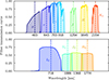 |
Fig. 1. Set of passbands describing the photometry of mock red quasars. The panels show the transmission efficiencies for the broad-band optical DECam griz filters, the Euclid VIS (optical) and NISP (NIR) filters, and the NIR to MIR VISTA JHKs filters. The vertical dashed lines are placed at the weighted central wavelength of each filter. |
To create the mock catalogue, we used the synthetic quasar spectrum constructed in Euclid Collaboration: Lusso et al. (2024), where a sample of quasars from SDSS DR7 (Shen et al. 2011) was selected across redshifts and grouped into nine bins of full width at half maximum (FWHM) of the Hβ emission line (see Table 1 in Euclid Collaboration: Lusso et al. 2024). Specifically, quasars were organised into three equivalent-width (EW) intervals ([15, 30], [30, 60], ≥ 60 Å) and three FWHM intervals ([2000, 3000], [3000, 5000], ≤5000 km/s), yielding a grid of nine spectral stacks. Stitching together the stacked spectra, the authors created a composite spectrum with very broad wavelength coverage.
Figure 2 shows the unobscured quasar spectrum and the dramatic impact of E(B − V) = 0.25 attenuation applied to it. The coloured bars correspond to the rest-frame wavelength coverage of the red-grism of Euclid. To create a mock catalogue of red quasars, we used the first spectral stack from Euclid Collaboration: Lusso et al. (2024) and the luminosity function of red quasars black determined in Glikman et al. (2018). The latter is described by a double-power-law function, which was already presented in Lacy et al. (2015); this is characterised by a faint-end and a right-end slope and a break luminosity, where the dominance shifts from the faint to the bright end.
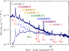 |
Fig. 2. Spectrum comparison between unobscured quasar stack (dark blue line; Euclid Collaboration: Lusso et al. 2024) and a reddened quasar spectrum with E(B − V) = 0.25 (light blue line). Emission lines are highlighted using coloured vertical markers along with their respective labels, pointing to different atomic species and ionisation states. The coloured bars correspond to the redshift range of the red grism of NISP. |
We created a grid of bolometric luminosity (40 < log10Lbol < 48, in erg s−1) and redshift (0 < z < 7) and calculated the expected number of red quasars by integrating the luminosity function. For each mock SED, we applied reddening according to their distribution covering 0.25 < E(B − V) < 1.45 and assuming the SMC attenuation law (Prevot et al. 1984) and intergalactic medium attenuation as described in Euclid Collaboration: Lusso et al. (2024). The chosen E(B − V) corresponds to the observed range in the sample of Glikman et al. (2018).
Finally, we applied an observed magnitude cut corresponding to the expected depth of EWS; i.e. J < 24.5. Figure 3 shows the coverage of the luminosity-redshift plane of our mock catalogue, assuming 14 500 deg2 sky coverage, at the wide-depth of Euclid. The black line shows the break luminosity of red quasars from Glikman et al. (2018).
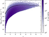 |
Fig. 3. Luminosity-redshift plane for mock sample of red quasars. The black line is the knee of the luminosity function of Glikman et al. (2018). |
2.2. COSMOS2020 sample
We used the COSMOS2020 dataset as our reference sample of observed sources. The catalogue includes multi-wavelength photometry spanning from the ultraviolet (UV) to the MIR, making it a suitable benchmark for assessing the separation of red quasars and other populations.
We cleaned the COSMOS2020 sample from corrupted photometry and fake detections and excluded the objects with null entries for the photometric redshift. To do this, we applied the mask FLAG_COMBINED = 0 to remove objects near bright stars and saturated regions, ACS_MU_CLASS = 1 to identify stars and remove them to retain galaxies, and lp_type ≠ 9 to exclude fake detections. Furthermore, we applied a magnitude upper cut at 23.5 in VISTA H in both COSMOS2020 and the mocks. Among the selected sources in the COSMOS2020 catalogue, we took into account those that are flagged as AGN candidates. The selected catalogue includes 95 052 objects.
Additionally, we excluded 1493 X-ray sources observed with Chandra (Civano et al. 2016) from our analysis. X-ray-selected AGNs outline a broad range of obscuration and their optical-to-NIR colours may not fully align with the selection criteria used in this study, which is based solely on red-quasar NIR photometry. We note that this sub-sample of X-ray AGNs constitutes a small fraction of the COSMOS2020 dataset and is not expected to dominate the target red quasar population. Its inclusion will be valuable for future works (see Sect. 5.6), as their properties can be used to refine the distinction between reddened AGNs and red galaxies.
2.3. Template fitting for COSMOS2020
Each object in COSMOS2020 is described by a photometric dataset including UV measures from GALEX, optical observations from the Subaru Hyper Suprime-Cam (HSC) and the Canada-France-Hawaii Telescope (CFHT), NIR data from VISTA, MIR data from the SPLASH programme of the Spitzer Space Telescope, and optical medium-band observations from Subaru. We refer the reader to Weaver et al. (2022) for references on these individual datasets. The properties of each filter are described in Table A.1.
The mock dataset includes VISTA, DECam, and Euclid VIS and NISP photometry. In order to match the photometric datasets of mocks and COSMOS2020, we used template fitting (TF) to estimate the optical and NIR fluxes that were originally not available in the latter. TF compares the input photometric dataset with a library of spectral energy distributions (SEDs) to identify the best match. For this task, we used the Phosphoros package (Paltani et al., in prep). Phosphoros is a fully Bayesian TF algorithm, supporting flexible prior distributions across allparameters (redshift, reddening, SED index, and luminosity) and producing multi-dimensional and marginalized posterior distributions. It was successfully employed in the Euclid photo-zchallenge, presented in Euclid Collaboration: Desprez et al. (2020), which was designed to evaluate the accuracy of various methods for photometric redshift estimation against the stringent requirements of Euclid cosmic shear analyses (Cropper et al. 2013, Tarsitano et al., in prep.). In Desprez et al. (2023), Phosphoros was validated and benchmarked against a similar code, Le Phare (Arnouts & Ilbert 2011). For each input galaxy, Phosphoros provides a multi-variate posterior distribution, allowing the inference of flux estimates in the missing bands from the best fit. For additional details about its metrics and models we refer the reader to Desprez et al. (2023) and Euclid Collaboration: Tucci et al. (2026).
2.4. Euclid Q1 dataset
We analysed mocks and COSMOS2020 (methods are described in Sect. 3) to derive a selection function for candidate red quasars, and we applied it to Euclid Q1 (Euclid Collaboration: Mellier et al. 2025). Q1 consists of a first visit of the Euclid Deep Fields (EDFs), spanning across a total area of 63.1 deg2 of the extragalactic sky; this area is divided among the Euclid Deep Field North (EDF-N, 20 deg2), Euclid Deep Field Fornax (EDF-F, 10 deg2), and the Euclid Deep Field South (EDF-S, 23 deg2). More details about the Q1 release are presented in Euclid Collaboration: Aussel et al. (2026), Euclid Collaboration: McCracken et al. (2026), Euclid Collaboration: Polenta et al. (2026) and Euclid Collaboration: Romelli et al. (2026).
In this work, we focused on the EDF-F, for which we find overlap with a collection of AGN candidates from Zou et al. (2022) – selected through the flag flag_IRagn_D12 – which follows the MIR colour-based cut proposed in Donley et al. (2012), and a catalogue of radio-selected quasars (Miller et al. 2013). These two datasets were used as external reference samples to independently assess the reliability of the selection function. In this work, we refer to them as control samples, as they provide an observational benchmark for AGNs, including potentially obscured sources. Their purpose is to evaluate whether known AGNs, selected via independent criteria, are successfully recovered by our method. This comparison is valuable for assessing the completeness of our selection function and flagging potential biases. We built a first dataset of 5 301 332 EDF-F sources, obtained by matching the Euclid morphology (Euclid Collaboration: Romelli et al. 2026) and photometric redshift (Euclid Collaboration: Tucci et al. 2026) catalogues. Then, we excluded objects flagged as spurious and with unphysical photometric and redshift properties. Furthermore, we only considered sources classified either as galaxies or quasars, according to the classification assigned in the Euclid photometric redshift pipeline (Euclid Collaboration: Tucci et al. 2026). A summary of this selection function is reported in Table 1. Additionally, we applied a cut near the limiting magnitude of the HE band, corresponding to 23.5. The final sub-sample at play counts 1 331 325 sources.
Sample selection function applied to the Q1 sample.
3. Methods
Colour-based selection criteria were extensively studied in the literature to identify AGNs and reddened AGNs. Most notably, Lacy et al. (2004), Stern et al. (2005), Mateos et al. (2012), and Assef et al. (2018) defined empirical cuts in MIR colour space. Alongside MIR-based selections, NIR colours have been proposed in Banerji et al. (2012) and Glikman et al. (2012, 2013, 2018), to separate red quasars from stars and galaxies.
To follow-up on these studies exploiting the unique depth and high-resolution of Euclid, we introduce a novel selection method that is solely based on Euclid NIR photometry. Our goal is to enhance the systematic identification of red quasars in the EWS where MIR photometry may be incomplete or unavailable.
To achieve this, we conducted a series of statistical analyses to study the photometric selection criteria that maximise the separation between the COSMOS2020-observed dataset and the mock red quasars. In particular, we explored the separation in a multi-dimensional colour-colour space, as a function of magnitude and redshift. Our study was performed independently using VISTA+DECam and reconstructed Euclid photometry. This allowed us to assess the impact of different wavelength coverage and filter sets on the identification of red quasars and to evaluate the Euclid NIR stand-alone capability of recovering our target population.
First, we collected features that are directly transferable into the reconstructed Euclid-like photometry. More precisely, we considered VISTA J − Ks, Y − Ks and J − H to describe NIR colours, and DECam i − Ks to sharpen the selection of reddened sources based on their optical-to-NIR transition. In the Euclid-like colour space, we used YE − HE, JE − HE, and YE − JE as NIR colours, and we adopted IE − HE as a metric to estimate the optical-to-NIR excess. We proceeded with the implementation of a multi-step analysis, which is detailed as follows:
-
Principal component analysis (PCA): This method has been successfully applied in previous studies to investigate the underlying physical properties of AGNs and their host galaxies. Boroson & Green (1992) were the first to use it in the AGN domain, to analyse optical emission lines and continuum properties of a low-redshift quasar sample. Their work was followed by Corbin (1993), Laor et al. (1994, 1997), Wang et al. (1996), and Brandt & Boller (1998). Their analyses found correlation between the primary eigenvector (or principal component) and quasar spectral features depending on physical parameters including Eddington ratio, luminosity, and black-hole spin. Beyond optical emission lines, the PCA has been applied to AGN spectral energy distributions and photometric datasets. Yip et al. (2004) applied PCA on SDSS quasar spectra and showed that the eigenvectors (named eigenspectra in their work) have the power to disentangle the contribution of the host-galaxy light, the optical continuum, and the AGN emission. Kuraszkiewicz et al. (2009) analysed a sample of red 2MASS AGNs (Cutri et al. 2002). Among their results, they found that the second principal component was correlated with optical-to-infrared colours (B − Ks, B − R, J − Ks), depending on the contribution of the host galaxy relative to the AGN emission. PCA was also used to study AGN samples in Hao et al. (2005), Stern & Laor (2012), Panda & Śniegowska (2024). In this work, we applied a PCA to the aforementioned multi-dimensional colour space to identify the most informative colours that separate mock red quasars from the observed COSMOS2020 sources. Our analysis focuses on broadband photometric selection in preparation for systematic large-scale red quasar searches in the Euclid Survey. Through a linear combination of the original features, a PCA reduces dimensionality while capturing variance in the dataset. It serves as an exploratory framework to highlight which optical and NIR colours contribute most to the identification of red quasars. Detailed information follows in Sect. 3.1.
-
Empirical colour-colour cuts: Using the most significant colours identified via the PCA, we studied a colour-colour selection function for red quasars. Additional information on the metric adopted to evaluate the selection performance is reported in Sect. 3.2.
-
Machine learning-based refinement: In this phase, we trained a probabilistic random-forest classifier (RF; Breiman 2001) to refine the previous selection function for red quasars and mitigate the effects of contaminants. RF has the advantage of handling non-linear relationships between the input features, so it sets complex decision boundaries that a PCA and empirical colour-based cuts cannot capture. The trained RF model was then applied to the Euclid Q1 dataset, where we selected candidate red quasars based on their predicted probabilities. We refer readers to Sect. 3.3 for a detailed description of this method.
In the analysis, we considered the discriminating power of additional features, such as compactness criteria, and we used external AGN datasets as control samples. The latter play a crucial role in identifying the proposed selection function and assessing its robustness, or revealing the risk of introducing a bias that could reduce the completeness of the red quasar selection. We used our findings to build a first census of candidate red quasars in Euclid Q1 EDF-F. Such a sample provides a framework for future spectral analyses and will serve as a training set for artificial-intelligence-based automated classification, extended to the EDF-N, EDF-S, and EWS.
3.1. Hyper-colour determination and colour selection
A PCA is a statistical method that can be used to project a dataset from a high-dimensional space into a low-dimensional space, retaining its most meaningful properties. More precisely, the technique consists of mapping the original features into a new set of uncorrelated ones, named principal components. The result is a linear combination where each coefficient represents the contribution of the corresponding original feature in forming a principal component. With this technique, the dataset is linearly transformed onto a new coordinate system whose directions – the principal components – capture as much variance in the data as possible, with the first component capturing the most variance, the second capturing the next most, and so on.
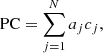
In this work, we used the module PCA available in the Python library Scikit-learn (Pedregosa et al. 2011), which follows the implementation presented in Halko et al. (2009). Applying PCA decomposition to our multi-dimensional dataset, described by the aforementioned colour features, means collapsing it into a low-dimensional one, where each principal component (PC) is a linear combination of the original colours (c):
 (1)
(1)
with aj being the coefficients of the linear combination, and N, the number of involved colours. Features with consistently high coefficients across components explain a larger portion of the variance and are more important in the transformed space. The aim is to identify principal components receiving significant contributions by a set of original colours and study their discriminating power between red quasars and the rest of the sample. We refer to such principal components as hyper-colours (HCs).
We ran a PCA on the mocks and COSMOS2020, standardising the input features to ensure comparability across different scales. By assuming three principal components, we identified a cut in the HC space that guarantees the highest discriminating power. We refer to this as the HP cut.
Furthermore, we studied the impact that the single colour features, cj, have on the HCs, based on their linear coefficients aj, and we identified a cut in the multi-dimensional colour-colour space made by them. We refer to this selection cut as a colour-colour (CC) cut.
3.2. Forecast analysis
By applying the HP or CC cut, we estimate the completeness (C) and purity (P) of the selected sample. Completeness is the fraction of mock red quasars correctly identified by the proposed selection criterion and is defined as
 (2)
(2)
where true positives (TPs) and false negatives (FNs) are the number of red quasars correctly identified and missed by the cut, respectively. The sum TP + FN thus corresponds to the total number of red quasars in the mock sample. Purity is defined as the fraction of TPs among all selected objects. We calculated it as
 (3)
(3)
where false positives (FPs) are the number of sources incorrectly identified as red quasars by the selection cut. In this work, we define FPs as the number of COSMOS2020-selected sources that are not classified as AGNs, plus the number of AGN candidates passing the cut with DECam i − Ks < 1.7. We assumed this metric since 1.7 is the lower limit for optical-to-NIR excess in the mock sample. Finally, we applied the colour-based selection functions to EDF-F, and we studied them with the aid of two control samples of MIR-selected and radio-selected AGN candidates in the same field.
3.3. Probabilistic random forest
A RF is a machine-learning algorithm that consists of creating an ensemble of decision trees and combines their outputs to make predictions. Each tree in the forest is trained on a random subset of the data and features, and the final classification is done by majority voting (standard RF) or by averaging the predicted probabilities assigned to each class across all the decision trees (probabilistic RF). In a binary classification case, a probabilistic RF assigns each source two values, corresponding to their probability of belonging to each of the two classes. This approach allows us to estimate the confidence level of each classification and make a probabilistic selection of candidate red quasars. The RF method can identify and rank the most important features that differentiate red quasars from other objects, and it can handle complex and non-linear relationships between features. Furthermore, RF is more robust in terms of over-fitting, which makes it suitable for noisy or imbalanced datasets, as in the case of targeting red quasars (Breiman 2001; Chen et al. 2004). In our work, we used the module RandomForestClassifier available in the Python library Scikit-learn.
First, we trained a RF classifier on three sets of features (named S1, S2 and S3) based on different combinations of Euclid-based colours and magnitudes. More precisely, S1 includes the most significant colours identified by PCA, and S2 includes all the Euclid NIR colours. S3 includes both Euclid NIR colours and magnitudes. This multi-step approach allowed us to test the impact of expanding the primary feature set in terms of purity, completeness, and classification performance.
For each set of features, we identified the best model using hyper-parameter tuning. The RF model operates within a hyper-parameter space described by a set of key parameters, whose combinations can impact the performance of the model itself. These parameters include the number of trees, the minimum amount of samples required to split a tree node (i.e. a point in the tree where the data is split based on the value of a certain input feature), and the leaf size (i.e. the minimum number of samples required to be in a leaf, which is a terminal node making a final prediction). We used the Scikit-learn module RandomizedSearchCV to explore this hyper-parameter space and identify the best performing set of key parameters. For each sampled combination of parameters, the algorithm employs a stratified k-fold cross-validation strategy with k = 5 folds. This technique divides the dataset into five partitions and trains the model on four of them, using the fifth for validation. The goal of this approach is to achieve a robust estimate of the model performance and check if over-fitting occurs at certain partitions. The best combination of parameters is selected based on the cross-validation accuracy.
Through hyper-parameter tuning and cross-validation (run with a fixed random seed for reproducibility), we obtained an optimised RF model for each initial set of features (S1, S2, and S3). We compared the three models in terms of feature importance, completeness, and purity, and we applied the best one to the Euclid Q1 EDF-F dataset. We discuss the results and our findings in Sect. 4.
4. Results
The main goal of this work is to identify a robust sample of candidate red quasars in the Euclid Q1 dataset. As described in Sect. 3, we adopted a multi-step approach involving PCA, colour-colour cuts, and machine-learning classification. In this section, we present results of each step and evaluate their effectiveness in isolating the target population.
4.1. Selection function in the HC space
The PCA on mocks and COSMOS2020, run in VISTA-defined multi-dimensional colour space, provides three HCs whose coefficients are reported in Table A.2. HC1 is a weighted average of all the input colour features, with a slight emphasis on J − Ks and i − Ks. HC2 and HC3 are dominated by H − Ks and i − Ks. Their explained variances (91%, 6.2%, and 2.7%, respectively) indicate that HC1 is related to the overall colour gradients across the feature set, while HC2 and HC3 isolate information specific to a certain feature. The combination of HC1 and HC3 provides the strongest discriminating power, as displayed in Fig. 4. The contours, normalised to their respective subsets, show that this HC space is able to effectively disentangle the populations of mock red quasars from the observed sources in COSMOS2020. The latter includes both galaxies and AGN candidates, as described in Sect. 2. The HC cut of HC1 > 0.6 and HC3 > −0.9 leads to an overall completeness level of 98%, with 81% purity. Among the COSMOS2020 AGN candidates passing the cut, 91% of them have DECam i − Ks > 1.7. As reported in Sect. 3, based on mocks we considered this as a requirement to identify possible obscured AGNs and flag them as candidate red quasars.
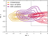 |
Fig. 4. Hyper colour-colour diagram obtained using VISTA+DECam photometry, showing the separation of mock red quasars from COSMOS2020 sources. The latter include galaxies (gold contours) and AGN candidates (in purple). The contours are normalised to their respective subsets. The proposed selection function is displayed via the grey dashed lines. |
We ran the PCA again, transferring the original VISTA colour features into the Euclid-like colour space, yielding similar results. The coefficients of the principal components are displayed in Table A.3. Analogously to the VISTA-based HCs, the Euclid-based HC1 is dominated by YE − HE, and HC3 obtains most contribution from IE − HE, tracking the optical-to-NIR transition. Figure 5 displays the Euclid-like HC space formed by HC1 and HC3. An HC cut of HC1 > 0.3 and HC3 > −0.9 leads to an overall completeness level of 97% with 68% purity.
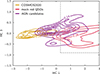 |
Fig. 5. Hyper colour-colour diagram obtained using Euclid-like photometry, showing separation of mock red quasars from COSMOS2020 galaxies (gold contours) and AGN candidates (in purple). The proposed selection function is displayed via the grey dashed lines. |
Beyond unveiling hyper-colours, the PCA highlights the original colour features, cj in Eq. (1), bringing the most weight in the identification of candidate red quasars. More precisely, in the VISTA parameter space, the most important colours for HC1, HC2 and HC3, based on their linear coefficients, are J − Ks, H − Ks, and i − Ks. In the Euclid-like parameter space, the most important features for the tree components are YE − HE, JE − HE, and IE − HE, respectively. We further advanced our analysis with a visual and quantitative assessment of the separation of mock red quasars using these multi-dimensional colour-colour spaces.
4.2. Photometric selection in colour-colour space
Figure 6 displays the separation between mock red quasars and the COSMOS2020 dataset achieved in a multi-dimensional parameter space spanning from optical to NIR wavelengths and defined through the most important colour features according to the PCA. The two populations are compared in the J − Ks versus H − Ks diagram, and COSMOS2020 is further split in two subsets to highlight candidate AGNs. If we apply the cut J − Ks > 0.8 and H − Ks > 0.2, we obtain an overall completeness level of 99% and a purity of 78%. We find that 85% of the candidate AGNs passing this multi-dimensional colour cut responds to the mock-calibrated red excess of DECam i − Ks > 1.7.
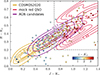 |
Fig. 6. VISTA+DECam colour-colour diagram showing separation of mock red quasars from COSMOS2020 galaxies (gold contours) and AGN candidates (in purple). The proposed selection function is displayed by the grey dashed lines. A subset of COSMOS2020 candidate AGNs overlays the selection, colour-coded as i − Ks. |
As the CC cut is defined through optical and NIR colours, the purity estimate can be influenced by dependences on redshift and magnitude. We first estimated purity as a function of redshift. In Fig. 7, we show the separation between the COSMOS2020 sample and mock red quasars as a function of redshift, based on the most relevant features (J − Ks and i − Ks). We obtain 90% purity at z < 0.5, 69% at 0.5 < z < 1.5, and 87% at higher redshifts. The observed trend arises from colour degeneracies between red quasars and massive red galaxies. We refer the reader to Sect. 5.1 for a more detailed discussion of these effects. The magnitude dependency sees purity values of 77% for H < 20, 65% for 20 < H < 22 and 86% for objects in the interval 22 < H < 23.5.
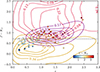 |
Fig. 7. VISTA+DECam colour-z diagram showing the separation of mock red quasars from COSMOS2020. The colour-codes adopted for the displayed populations are as in Fig. 6. |
We proceeded with the forecast analysis using the same metric, but defined with Euclid-like photometry. We studied a grid of multi-dimensional CC cuts to maximise the separation between the subsets at play, and we weighted the FP rate with the unreddened COSMOS2020 AGN candidates. The results are displayed in Fig. 8, with the colour-redshift evolution shown in Fig. 9. In this case, we find that the colour cut, YE − HE > 0.7 and JE − HE > 0.3 with IE − HE > 1.8, leads to an overall 99% completeness level and 67% purity, with redshift-dependent fluctuations: 86% purity at z < 0.5, 57% and 63% at 0.5 < z < 1.5 and higher redshifts, respectively. Purity values with magnitudes are 56% for HE < 20, 50% for 20 < HE < 22, and 77% for objects in the interval 22 < H < 23.5.
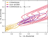 |
Fig. 8. Euclid-like colour-colour diagram showing separation of mock red quasars from COSMOS2020. The proposed colour-colour selection function is displayed via the grey dashed lines. The COSMOS2020 sample passing the selection is displayed in purple. |
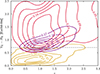 |
Fig. 9. Euclid-like colour-redshift diagram showing separation of mock red quasars (in red) from COSMOS2020 (golden contours). The COSMOS2020 passing the proposed CC cut is displayed in purple. |
4.3. Colour-colour selection applied to Euclid Q1
Having established the methods for the selection of red quasars based on mock and observed training samples in the previous sections, we then applied these methods to the Euclid Q1 EDF-F dataset. The selection is supported by control samples; MIR-selected and radio-selected AGN candidates, introduced in Sect. 2. Figure 10 display the discriminating power of the multi-dimensional CC cut, yielding an overall 98% completeness level of the mock sample. The colour-redshift evolution is displayed in Fig. 11. The MIR-selected and radio-selected AGNs have 77% and 47% reddened sources, according to the proposed cut IE − HE > 1.8. Among them, 87% pass the multi-dimensional CC cut. The selection functions are summarised in Table 2. Combining the CC cut with the RF classification probability (described in Sect. 3), we flag 151 853 sources as candidate red quasars.
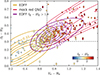 |
Fig. 10. Colour-colour diagram showing separation of mock red quasars from the Euclid Q1 sample. The proposed colour-colour selection is displayed via the grey dashed lines. The control samples are colour-coded by IE − HE; dots and diamonds represent MIR-selected and radio-selected AGNs, respectively. |
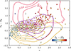 |
Fig. 11. Colour-z diagram showing separation of mock red quasars from the Euclid Q1 sample. The proposed colour-colour selection is displayed by the grey dashed line. The control samples are colour-coded by IE − HE; dots and diamonds represent the MIR-selected and radio-selected AGNs, respectively. The contours are coloured as in Fig. 10. |
Forecast red quasars’ completeness (C) and purity (P) from NIR selection functions.
4.4. Random-Forest analysis
In the previous steps of the analysis, we used a PCA to identify which regions in the hyper-colour space are most effective in distinguishing red quasars from other populations. Furthermore, using the most significant features based on PCA, we defined a three-dimensional colour-selection function, achieving high completeness levels and moderate purity (see Table 2).
In this final stage of the analysis, we aim to refine our selection using a probabilistic RF classifier. As discussed in Sect. 3.3, a RF can capture non-linear decision boundaries in the feature space, which are not detected by PCA or empirical CC cuts. This makes RF well-suited to increasing the purity of the selected sample of red quasars.
We applied a probabilistic RF classifier to identify candidate red quasars starting from a first set of photometric features, S1, including the most significant colours according to PCA: JE − HE, YE − HE, and IE − HE. The hyper-parameter search lead to an optimised model with 100 trees, minimum split size of 10, and minimum leaf size equal to 1. This configuration yields a mean cross-validation accuracy level of 95%, with a standard deviation of < 1%. We recover feature-importance values of 0.35 for JE − HE, 0.39 for YE − HE, and 0.26 for IE − HE.
Applying a probability threshold of P > 0.7 for classification, we obtain a 98% completeness level and 87% purity. We determined the probability threshold so that the completeness did not fall below the value we achieved using empirical CC cuts. This criterion ensures that the RF classification is at least as conservative as the other selection methods while improving purity.
To gather further insights from our analysis, we employed the uniform manifold approximation and projection algorithm (UMAP). As described in McInnes et al. (2018), the UMAP is a non-linear dimensionality-reduction technique that preserves both the local and global structure of the data and highlights possible clusters and patterns. We used UMAP to visualise the dataset in a reduced-dimensionality space and check the separation between classes.
The UMAP visualisation of the classified objects (Fig. 12), colour-coded by probability of being a red quasar, shows that a threshold of 0.7 outlines a boundary region between the two classes. One hundred sources randomly drawn from the test set are plotted over the map, with symbols following the empirical CC cut. Stars are used for sources classified as red quasars, and circles represent sources that did not pass the selection. The overlay displays a direct comparison between the empirical colour-selection method and the RF classification. Previously selected sources are mostly present in the region a with higher probability of being a red quasar and a minority populates the transition region. The RF refinement of these boundaries goes beyond the level of accuracy achieved by the empirical CC cut, thereby reducing contamination and raising purity.
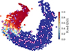 |
Fig. 12. UMAP visualisation for the results of the probabilistic RF classifier run on the most significant colour features based on PCA. Hexagons are colour-coded by probability of being a candidate red quasar. The overlaid scatter plot displays a random subset with symbols reflecting the empirical CC cut. Stars represent objects previously classified as red quasars. Circles are employed otherwise. |
We repeated the analysis on extended sets of features, specifically on S2 and S3 (introduced in Sect. 3.3), in order to assess the impact of additional information on the classification performance. More precisely, S2 includes YE − JE, JE − HE, YE − HE, and IE − HE, while S3 builds upon S2 by including in the set of features the magnitudes IE, YE, JE, and HE. The RF classifier optimised for S2 yields similar results, without improving completeness and purity. The feature-importance analysis assigns to the additional colour, YE − JE, a value of 0.03. Such results align with our findings from S3. In this case, the importance of the magnitude features is < 2%, and no increase in completeness and purity is registered.
Along this multi-step analysis, the dominant importance of the PCA-selected colours remains unchanged and leads to a consolidated probabilistic RF model that we applied to the Euclid Q1 EDF-F sample.
The UMAP visualisation of the Euclid Q1 sample, displayed in Fig. 13, is colour-coded by probability of being a red quasar. The over-plotted symbols represent a fraction (25%) of the two control samples: circles denote the MIR-selected AGN candidates, while diamonds represent the radio-selected AGN candidates. White markers indicate the sources that passed the previous empirical CC cut selection, and light grey colours those that were not classified as red quasars. Analogously to our findings from the analysis of the COSMOS2020 dataset, we notice that the spatial distribution of the sources is clustered around two different populations (according to their likelihood of being red quasars) and that the boundaries obtained via RF are more robust to contaminants, compared to the empirical CC cuts.
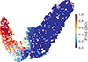 |
Fig. 13. UMAP visualisation of Euclid Q1 dataset, colour-coded by the RF-based probability of being a red quasar. The overlaid scatter plot displays 25% of the validation samples. MIR and radio-selected candidate AGNs are marked by circles and diamonds, respectively. The symbols are filled in white if the source passed the empirical CC cut; otherwise, they are coloured in light grey. |
5. Discussion
In this section, we comment and expand on our findings presented above, discussing the performance of the proposed selection function, the refinement using probabilistic RF, and the added value of the Euclid data through morphological and colour analyses. We also discuss potential future extensions, including dual AGN identification and spectroscopical analyses.
5.1. Performance of the selection function
The VISTA-based HC spaces provide effective separation between mock red quasars and observed sources. Their translation into the Euclid-like HC space preserves the structure of the primary component (HC1), while introducing small shifts in the secondary components (HC2 and HC3). These shifts are expected due to the differences in filter characteristics and photometric uncertainties. The photometric selection function, using multi-dimensional colour cuts in the Euclid optical and NIR regimes, forecasts high levels of completeness (98%) and moderate purity (78%) for candidate red quasars. The completeness of the mocks remains consistently high across redshift and magnitude intervals, suggesting that the proposed selection effectively captures the reddened quasar population. Purity decreases in intermediate redshift ranges and at faint magnitudes, where physical degeneracies between red quasars and red galaxies become more significant. However, comparing redshift and magnitude distributions of the mock red quasars and the sources in COSMOS2020 suggests there is also an observational effect at play. Figure A.1 shows that the redshift distribution of mock red quasars peaks at higher values compared to the observed sources, as they are modelled to represent a deeper survey aiming to capture the properties of obscured AGNs. Purity estimates can be affected in the mismatched higher redshift range. The lower purity at intermediate redshift could be partially mitigated by training the selection function on larger, more representative datasets that include additional sources of variation, such as differences in host-galaxy properties or environmental factors. Future work could explore the inclusion of environmental parameters, such as local density or clustering, to refine selection criteria. Larger values of purity for bright objects is also influenced by the broader photometric extent of Euclid-like mocks, which outnumber COSMOS2020 at lower magnitudes (Fig. A.2). On the opposite side, fainter sources are more prone to contamination by non-AGN populations due to increasing photometric uncertainties, an aspect that potentially reduces purity at fainter magnitudes.
5.2. Considerations on the mock-based approach
In our analysis, we used a red quasar mock catalogue based on the stacking of SDSS quasar spectra with varying levels of reddening applied. While this approach effectively models the intrinsic quasar properties, it does not account for the host-galaxy contamination. The host-galaxy flux can dominate over the AGN emission in the optical and NIR bands, especially for lower redshift sources. The consequent dilution of quasar colours may reduce the effectiveness of our HC selection criteria, which are primarily optimised for quasar-dominated SEDs. Such aspects set the seed for future works, where our mock catalogue incorporates realistic galaxy templates, either by adding scaled galaxy SEDs to the quasar spectra or by using simulations informed by empirical measurements of quasar host properties. Nevertheless, our analysis still provides valuable insights into the potential of Euclid when it comes to identifying red quasars. As reported in Sect. 4, we also note that our results remain robust for brighter sources (H < 22), which are aligned closer to SDSS, where the impact of host galaxies is expected to be minimal.
5.3. Optimisation of the selection function with probabilistic RF
The probabilistic RF classifier refines the empirical CC cut by achieving higher levels of completeness and purity (98% and 88%, respectively). This improvement is due to the RF ability to integrate non-linear relationships in the multi-dimensional feature space, which are not detected with simpler colour-colour cuts.
A key aspect in our RF approach is that is starts from a set of features including the most significant colours, according to PCA, and then expand it with additional colours and magnitudes. Through feature-importance analysis, this multi-step methodology allows us to assess how the classification performance is impacted by the information encoded in the additional features. Furthermore, such expansion did not lead to substantial improvements in completeness and purity, confirming the NIR multi-dimensional colour space (JE − HE, YE − HE, and IE − HE) as the most informative and effective to classify out target population.
The UMAP visualisation of the datasets, colour-coded by probability of a source being a red quasar, shows that the threshold P > 0.7 effectively segments the transition region between the two classes. In comparison with the overlaid validation datasets, it shows consistency and robustness against contaminants.
5.4. Visual assessment of the morphology and environment of candidate red quasars
To further clarify our selection, we made an initial visual assessment of the morphological properties of the candidate red quasars. The visual inspection of the selected sources reveals that most candidates exhibit point-like or slightly extended profiles, consistent with AGN-dominated systems. The multi-wavelength images in the first three panels of Fig. 14 show sources with bright NIR emission and a weaker component in the VIS band, consistent with significant optical light attenuation due to dust. These characteristics suggest that the sources are indeed candidate red quasars. In this case, we also highlight the importance of this dataset for future morphological analyses, performing host galaxy decomposition and adding information on the properties of the AGN component and its dusty cocoon.
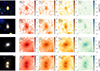 |
Fig. 14. Candidate red quasars. Panels show, from left to right, the RGB image and the HE, JE, YE, and IE bands. Raw images were obtained through ESA Datalabs (Navarro et al. 2024). |
In addition to examples of individuals red quasar candidates, in the fourth panel of Fig. 14 we introduce an example of a candidate dual-AGN system. The image displays two distinct compact sources with optical-to-NIR colour IE − HE = 2.4, at redshifts of 0.86 (central source) and 0.9; these are classified as candidate red quasars with RF-based probabilities of 0.82 (central source) and 0.74. Their proximity consists of a projected distance of less then 100 kpc and a difference in redshift not surpassing 0.06. Such criteria align with the definition of a dual AGN given in earlierliterature (De Rosa et al. 2019). Such systems offer a unique observational window into AGN triggering mechanisms, galaxy mergers, and the evolution of supermassive black holes. The example presented in this work will be part of future systematic searches of dual-AGN systems. This effort will use morphological analysis and spectroscopic follow-up, where available. The results of this investigation will be presented in forthcoming publications.
5.5. Comparison with VISTA+DECam-based selection
We expanded this first characterisation of the selected sources, making a comparison between candidates selected through VISTA and DECam colours and via Euclid-only colours. In the EDF-F, we identified a sample of 43528 objects observed by Euclid, the Vista Hemisphere Survey (VHS, McMahon et al. 2019), and DES. Among them, we selected 3% and 4% using solely Euclid and VISTA+DECam colours, respectively.
As shown in Fig. 15, Euclid-only-selected objects extend into redder IE − HE values. This suggests that Euclid is better at identifying the reddest sources, which might be missed by VISTA. Furthermore, we observe that the candidates identified through the VISTA+DECam system display a broader distribution towards bluer colours. This can be explained by VISTA depth and resolution, which are both inferior to Euclid, leading to misclassification and missing reddened sources. This preliminary analysis suggests that Euclid’s better resolution and NIR sensitivity enables a more complete and robust identification of red quasars.
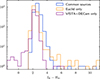 |
Fig. 15. Optical-to-NIR colour distributions for EDF-F sample of candidate red quasars observed through both Euclid and VISTA+DECam photometry. The orange and purple distributions are for candidates selected only via Euclid and VISTA+DECam colours, respectively. |
Figure 16 displays two examples of visually inspected candidate red quasars identified with colour selection based on either Euclid or VISTA+DECam only. These sources illustrate typical trends we observed across the sample, including enhanced compactness and contrast in the Euclid bands. More precisely, the first row of Fig. 16 shows an example of a red-quasar candidate selected with Euclid only. The image in the IE band shows a compact source with a bright centre and some faint surrounding structure which can be attributed to the quasar host galaxy. The presence of asymmetry in the outer structure hints at a merger history or disturbed morphology. The Euclid HE-band image shows a smooth compact core with higher emission than in the optical. This proves that the optical-to-NIR contrast is high. The VISTA and DES images are noisier, and the source is harder to distinguish. The poorer signal can explain why the VISTA+DECam system did not classify this sources as a candidate red quasar. Images are normalised and shown in flux units.
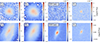 |
Fig. 16. Examples of two candidate red quasars. The first and the second rows show an Euclid-only and VISTA+DECam-only-selected candidate, respectively. Panels from left to right display the object in the IE and HE filters, in DECam i and VISTA Ks. |
We repeated the visual inspection on sources that were selected as candidate red quasars through the VISTA+DECam system only. In the second row of Fig. 16, the Euclid IE band displays an extended morphology with clear structures, possibly star-forming regions or satellite companions. In the DECam i band only the overall structure is less visible due to the lower resolution compared to Euclid. Similarly, in the VISTA bands the galaxy is less resolved and appears to be more concentrated in NIR. In this case, the lower resolutions of DECam and VISTA make the system look more compact, while Euclid sees a more extended morphology with detailed substructural features. Therefore, the VISTA+DECam colours used for the selection can be biased towards the integrated light of the system rather than its true morphology. This suggests that the Euclid-selected sample of red quasars tends to be cleaner, avoiding extended galaxies being misclassified as quasars.
5.6. Implications for future studies
In this work, we flagged over 150 000 sources in the EDF-F as candidate red quasars. This population serves as a first base for future refinements, incorporating additional diagnostics such as MIR data, spectral analyses (spectra were not considered in this work), and morphological compactness. Thesefeatures should help to further improve purity without compromising completeness. In terms of number expectations, we refer to the studies by Euclid Collaboration: Bisigello et al. (2024) and Euclid Collaboration: Selwood et al. (2025), which were conducted in anticipation of the Q1 data release. The former predicts a fraction of 57% AGNs among NIR-selected sources in EDF-F. The latter estimates an obscured fraction of 26% in the expected AGN population. Applying these forecasts to our EDF-F sample, we calculate 196 992 expected obscured AGNs. This is compatible with our selected sample, which is set to include reddened AGNs, a contamination of red galaxies, and red quasars. The classification of these sources will be the subject of future refinements based on the aforementioned criteria.
In this work, we excluded X-ray sources from the COSMOS2020 sample. However, their integration will be beneficial to future analyses, as their properties are directly linked to the degree of obscuration (Ma et al. 2024). This approach, which can be tested against the Q1 catalogue of X-ray AGN counterparts by Euclid Collaboration: Roster et al. (2026), can help improve the distinction between truly reddened AGNs from red galaxies, thereby improving the purity of the selected sample.
6. Conclusions
In this work, we explored the capability of selection criteria based on Euclid optical and NIR photometry to identify and characterise red quasars. We explored the separation in a multi-dimensional colour-colour space, as a function of magnitude and redshift, and we compared it with selections based on VISTA+DECam photometry. Through a joint PCA and statistical analysis we identified selection functions achieving high completeness levels and moderate purity. Then, to refine the identification of red quasars, we used a probabilistic RF classifier, which significantly improved purity (88%) and maintained a high level of completeness (98%). This result reflects the capability of this method to identify complex, non-linear relationships in a multi-dimensional colour space, beyond the reach of simple empirical cuts. Additionally, visualisation methods such as UMAP confirm a clear separation between red quasars and contaminants, reinforcing the robustness of our selectioncriteria.
Our analysis has shown that Euclid-based selection recovers redder quasar candidates than those identified by VISTA+DECam, as evidenced by shifts in the IE − HE distribution. This suggests that Euclid’s superior depth and resolution enable a more complete detection of highly obscured sources, which might be misclassified or missed in lower resolution surveys. Conversely, we found that some VISTA+DECam-selected sources appear as extended galaxies in Euclid images, indicating that lower resolution surveys may introduce contamination by compact galaxies in the sample of red quasars.
A key insight from future morphological inspection of the selected candidates will come from investigating the capability of Euclid to resolve host-galaxy features in a subset of sources, distinguishing between true quasars and compact galaxies.
We used our findings to build a first census of candidate red quasars in Euclid Q1. The catalogue will be released as a fits table to the Euclid Collaboration. This work provides the foundation for systematic red quasar searches in the Euclid Wide Survey (EWS). The proposed selection function will be further refined with additional diagnostics, including MIR data, spectroscopic follow-ups, and analysis of the host morphology. This first census of red-quasar candidates in Euclid Q1 represents a significant step towards a more complete understanding of the dusty AGN population and its connection to galaxy evolution.
Acknowledgments
This work has made use of the Euclid Quick Release (Q1) data from the Euclid mission of the European Space Agency (ESA), 2025, https://doi.org/10.57780/esa-2853f3b. The Euclid Consortium acknowledges the European Space Agency and a number of agencies and institutes that have supported the development of Euclid, in particular the Agenzia Spaziale Italiana, the Austrian Forschungsförderungsgesellschaft funded through BMK, the Belgian Science Policy, the Canadian Euclid Consortium, the Deutsches Zentrum für Luft- und Raumfahrt, the DTU Space and the Niels Bohr Institute in Denmark, the French Centre National d’Etudes Spatiales, the Fundação para a Ciência e a Tecnologia, the Hungarian Academy of Sciences, the Ministerio de Ciencia, Innovación y Universidades, the National Aeronautics and Space Administration, the National Astronomical Observatory of Japan, the Netherlandse Onderzoekschool Voor Astronomie, the Norwegian Space Agency, the Research Council of Finland, the Romanian Space Agency, the State Secretariat for Education, Research, and Innovation (SERI) at the Swiss Space Office (SSO), and the United Kingdom Space Agency. A complete and detailed list is available on the Euclid web site (www.euclid-ec.org). This work has made use of CosmoHub, developed by PIC (maintained by IFAE and CIEMAT) in collaboration with ICE-CSIC. CosmoHub received funding from the Spanish government (MCIN/AEI/10.13039/501100011033), the EU NextGeneration/PRTR (PRTR-C17.I1), and the Generalitat de Catalunya. This research makes use of ESA Datalabs (datalabs.esa.int), an initiative by ESA’s Data Science and Archives Division in the Science and Operations Department, Directorate of Science. The VISTA Hemisphere Survey data products served at Astro Data Lab are based on observations collected at the European Organisation for Astronomical Research in the Southern Hemisphere under ESO programme 179.A-2010, and/or data products created thereof. This work has benefited from the support of Royal Society Research Grant RGS\R1\231450. This research was supported by the International Space Science Institute (ISSI) in Bern, through ISSI International Team project #23- 573 “Active Galactic Nuclei in Next Generation Surveys”. F. R., B. L. acknowledge the support from the INAF Large Grant “AGN & Euclid: a close entanglement” Ob. Fu. 01.05.23.01.14.
References
- Almeida, C. R., & Ricci, C. 2017, Nat. Astron., 1, 679 [Google Scholar]
- Andonie, C., Alexander, D. M., Rosario, D., et al. 2022, MNRAS, 517, 2577 [NASA ADS] [CrossRef] [Google Scholar]
- Antonucci, R. 1993, ARA&A, 31, 473 [Google Scholar]
- Arnouts, S., & Ilbert, O. 2011, LePHARE: Photometric Analysis for Redshift Estimate, Astrophysics Source Code Library [record ascl:1108.009] [Google Scholar]
- Assef, R. J., Stern, D., Noirot, G., et al. 2018, ApJS, 234, 23 [Google Scholar]
- Banerji, M., McMahon, R. G., Hewett, P. C., et al. 2012, MNRAS, 427, 2275 [Google Scholar]
- Banerji, M., McMahon, R. G., Hewett, P. C., Gonzalez-Solares, E., & Koposov, S. E. 2013, MNRAS, 429, L55 [Google Scholar]
- Banerji, M., Alaghband-Zadeh, S., Hewett, P. C., & McMahon, R. G. 2015, MNRAS, 447, 3368 [Google Scholar]
- Boroson, T. A., & Green, R. F. 1992, ApJS, 80, 109 [Google Scholar]
- Bower, R. G., Benson, A. J., Malbon, R., et al. 2006, MNRAS, 370, 645 [Google Scholar]
- Brandt, N., & Boller, T. 1998, Astron. Nachr., 319, 163 [Google Scholar]
- Breiman, L. 2001, Mach. Learn., 45, 5 [Google Scholar]
- Calistro Rivera, G., Alexander, D. M., Rosario, D. J., et al. 2021, A&A, 649, A102 [NASA ADS] [CrossRef] [EDP Sciences] [Google Scholar]
- Calistro Rivera, G., Alexander, D. M., Harrison, C. M., et al. 2024, A&A, 691, A191 [NASA ADS] [CrossRef] [EDP Sciences] [Google Scholar]
- Chen, C., Liaw, A., & Breiman, L. 2004, Using Random Forest to Learn Imbalanced Data, Technical Report 666, Department of Statistics, UC Berkley [Google Scholar]
- Civano, F., Marchesi, S., Comastri, A., et al. 2016, ApJ, 819, 62 [Google Scholar]
- Corbin, M. R. 1993, ApJ, 403, L9 [Google Scholar]
- Cropper, M., Hoekstra, H., Kitching, T., et al. 2013, MNRAS, 431, 3103 [Google Scholar]
- Croton, D. J. 2006, MNRAS, 369, 1808 [NASA ADS] [CrossRef] [Google Scholar]
- Cutri, R. M., Nelson, B. O., Francis, P. J., & Smith, P. S. 2002, in IAU Colloq. 184: AGN Surveys, eds. R. F. Green, E. Y. Khachikian, & D. B. Sanders, ASP Conf. Ser., 284, 127 [NASA ADS] [Google Scholar]
- Dark Energy Survey Collaboration (Abbott, T., et al.) 2016, MNRAS, 460, 1270 [Google Scholar]
- De Rosa, A., Vignali, C., Bogdanović, T., et al. 2019, New A Rev., 86, 101525 [NASA ADS] [CrossRef] [Google Scholar]
- Desprez, G., Picouet, V., Moutard, T., et al. 2023, A&A, 670, A82 [NASA ADS] [CrossRef] [EDP Sciences] [Google Scholar]
- Donley, J. L., Koekemoer, A. M., Brusa, M., et al. 2012, ApJ, 748, 142 [Google Scholar]
- Euclid Collaboration (Desprez, G., et al.) 2020, A&A, 644, A31 [EDP Sciences] [Google Scholar]
- Euclid Collaboration (Schirmer, M., et al.) 2022, A&A, 662, A92 [NASA ADS] [CrossRef] [EDP Sciences] [Google Scholar]
- Euclid Collaboration (Bisigello, L., et al.) 2024, A&A, 691, A1 [NASA ADS] [CrossRef] [EDP Sciences] [Google Scholar]
- Euclid Collaboration (Lusso, E., et al.) 2024, A&A, 685, A108 [NASA ADS] [CrossRef] [EDP Sciences] [Google Scholar]
- Euclid Collaboration (Cropper, M., et al.) 2025, A&A, 697, A2 [Google Scholar]
- Euclid Collaboration (Jahnke, K., et al.) 2025, A&A, 697, A3 [Google Scholar]
- Euclid Collaboration (Mellier, Y., et al.) 2025, A&A, 697, A1 [Google Scholar]
- Euclid Collaboration (Selwood, M., et al.) 2025, A&A, 693, A250 [Google Scholar]
- Euclid Collaboration (Aussel, H., et al.) 2026, A&A, 711, A1 (Euclid Q1 SI) [Google Scholar]
- Euclid Collaboration (McCracken, H., et al.) 2026, A&A, 711, A2 (Euclid Q1 SI) [Google Scholar]
- Euclid Collaboration (Polenta, G., et al.) 2026, A&A, 711, A3 (Euclid Q1 SI) [Google Scholar]
- Euclid Collaboration (Romelli, E., et al.) 2026, A&A, 711, A4 (Euclid Q1 SI) [Google Scholar]
- Euclid Collaboration (Roster, W., et al.) 2026, A&A, 711, A16 (Euclid Q1 SI) [Google Scholar]
- Euclid Collaboration (Tucci, M., et al.) 2026, A&A, 711, A5 (Euclid Q1 SI) [Google Scholar]
- Euclid Quick Release Q1 2025, https://doi.org/10.57780/esa-2853f3b [Google Scholar]
- Fabian, A. C. 2012, ARA&A, 50, 455 [Google Scholar]
- Fawcett, V. A., Alexander, D. M., Brodzeller, A., et al. 2023, MNRAS, 525, 5575 [CrossRef] [Google Scholar]
- Fotopoulou, S., Buchner, J., Georgantopoulos, I., et al. 2016, A&A, 587, A142 [NASA ADS] [CrossRef] [EDP Sciences] [Google Scholar]
- Georgakakis, A., Clements, D. L., Bendo, G., et al. 2009, MNRAS, 394, 533 [Google Scholar]
- Glikman, E., Urrutia, T., Lacy, M., et al. 2012, ApJ, 757, 51 [Google Scholar]
- Glikman, E., Urrutia, T., Lacy, M., et al. 2013, ApJ, 778, 127 [Google Scholar]
- Glikman, E., Simmons, B., Mailly, M., et al. 2015, ApJ, 806, 218 [Google Scholar]
- Glikman, E., Lacy, M., LaMassa, S., et al. 2018, ApJ, 861, 37 [NASA ADS] [CrossRef] [Google Scholar]
- Habouzit, M., Li, Y., Somerville, R. S., et al. 2021, MNRAS, 503, 1940 [NASA ADS] [CrossRef] [Google Scholar]
- Halko, N., Martinsson, P. G., & Tropp, J. A. 2009, arXiv e-prints [arXiv:0909.4061] [Google Scholar]
- Hao, L., Strauss, M. A., Tremonti, C. A., et al. 2005, AJ, 129, 1783 [Google Scholar]
- Heckman, T. M., & Best, P. N. 2014, ARA&A, 52, 589 [Google Scholar]
- Kim, D., & Im, M. 2018, A&A, 610, A31 [EDP Sciences] [Google Scholar]
- Klindt, L., Alexander, D. M., Rosario, D. J., Lusso, E., & Fotopoulou, S. 2019, MNRAS, 488, 3109 [Google Scholar]
- Kuraszkiewicz, J., Wilkes, B. J., Schmidt, G., et al. 2009, ApJ, 692, 1180 [NASA ADS] [CrossRef] [Google Scholar]
- Lacy, M., Storrie-Lombardi, L. J., Sajina, A., et al. 2004, ApJS, 154, 166 [Google Scholar]
- Lacy, M., Ridgway, S. E., Sajina, A., et al. 2015, ApJ, 802, 102 [NASA ADS] [CrossRef] [Google Scholar]
- Laor, A., Fiore, F., Elvis, M., Wilkes, B. J., & McDowell, J. C. 1994, ApJ, 435, 611 [NASA ADS] [CrossRef] [Google Scholar]
- Laor, A., Fiore, F., Elvis, M., Wilkes, B. J., & McDowell, J. C. 1997, ApJ, 477, 93 [Google Scholar]
- Laureijs, R., Amiaux, J., Arduini, S., et al. 2011, arXiv e-prints [arXiv:1110.3193] [Google Scholar]
- Ma, Y., Goulding, A., Greene, J. E., et al. 2024, ApJ, 974, 225 [NASA ADS] [CrossRef] [Google Scholar]
- Magorrian, J., Tremaine, S., Richstone, D., et al. 1998, AJ, 115, 2285 [Google Scholar]
- Mateos, S., Alonso-Herrero, A., Carrera, F. J., et al. 2012, in Half a Century of X-ray Astronomy, eds. I. Georgantopoulos, & M. Plionis, 148 [Google Scholar]
- McCracken, H. J., Milvang-Jensen, B., Dunlop, J., et al. 2012, A&A, 544, A156 [NASA ADS] [CrossRef] [EDP Sciences] [Google Scholar]
- McInnes, L., Healy, J., & Melville, J. 2018, arXiv e-prints [arXiv:1802.03426] [Google Scholar]
- McMahon, R. G., Banerji, M., Gonzalez, E., et al. 2019, VizieR On-line Data Catalog: II/359. [Google Scholar]
- Miller, N. A., Bonzini, M., Fomalont, E. B., et al. 2013, ApJS, 205, 13 [NASA ADS] [CrossRef] [Google Scholar]
- Navarro, V., del Rio, S., Diego, M. A., et al. 2024, in ESA Datalabs: Digital Innovation in Space Science, ed. A. Cortesi(Singapore: Springer Nature Singapore), 1 [Google Scholar]
- Padovani, P., Alexander, D. M., Assef, R. J., et al. 2017, A&A Rev., 25, 2 [NASA ADS] [CrossRef] [Google Scholar]
- Panda, S., & Śniegowska, M. 2024, ApJS, 272, 13 [NASA ADS] [CrossRef] [Google Scholar]
- Pedregosa, F., Varoquaux, G., Gramfort, A., et al. 2011, JMLR, 12, 2825 [Google Scholar]
- Petley, J. W., Morabito, L. K., Rankine, A. L., et al. 2024, MNRAS, 529, 1995 [NASA ADS] [CrossRef] [Google Scholar]
- Prevot, M. L., Lequeux, J., Maurice, E., Prevot, L., & Rocca-Volmerange, B. 1984, A&A, 132, 389 [Google Scholar]
- Rose, M., Tadhunter, C. N., Holt, J., & Rodríguez Zaurín, J. 2013, MNRAS, 432, 2150 [Google Scholar]
- Shen, Y., Richards, G. T., Strauss, M. A., et al. 2011, ApJS, 194, 45 [Google Scholar]
- Silk, J., & Rees, M. J. 1998, A&A, 331, L1 [NASA ADS] [Google Scholar]
- Stacey, H. R., Costa, T., McKean, J. P., et al. 2022, MNRAS, 517, 3377 [NASA ADS] [CrossRef] [Google Scholar]
- Stern, J., & Laor, A. 2012, MNRAS, 423, 600 [NASA ADS] [CrossRef] [Google Scholar]
- Stern, D., Eisenhardt, P., Gorjian, V., et al. 2005, ApJ, 631, 163 [Google Scholar]
- Temple, M. J., Banerji, M., Hewett, P. C., et al. 2019, MNRAS, 487, 2594 [Google Scholar]
- Urrutia, T., Becker, R. H., White, R. L., et al. 2009, ApJ, 698, 1095 [Google Scholar]
- Urrutia, T., Lacy, M., Spoon, H., et al. 2012, ApJ, 757, 125 [Google Scholar]
- Urry, C. M., & Padovani, P. 1995, PASP, 107, 803 [NASA ADS] [CrossRef] [Google Scholar]
- Wang, T., Brinkmann, W., & Bergeron, J. 1996, A&A, 309, 81 [NASA ADS] [Google Scholar]
- Weaver, J. R., Kauffmann, O. B., Ilbert, O., et al. 2022, ApJS, 258, 11 [NASA ADS] [CrossRef] [Google Scholar]
- Wethers, C. F., Banerji, M., Hewett, P. C., et al. 2018, MNRAS, 475, 3682 [Google Scholar]
- Whalen, K. E., Hickox, R. C., DiPompeo, M. A., Richards, G. T., & Myers, A. D. 2020, ApJ, 888, 71 [Google Scholar]
- Wright, E. L., Eisenhardt, P. R. M., Mainzer, A. K., et al. 2010, AJ, 140, 1868 [Google Scholar]
- Yip, C. W., Connolly, A. J., Vanden Berk, D. E., et al. 2004, AJ, 128, 2603 [Google Scholar]
- Yue, B. H., Best, P. N., Duncan, K. J., et al. 2024, MNRAS, 529, 3939 [NASA ADS] [CrossRef] [Google Scholar]
- Zou, F., Brandt, W. N., Chen, C.-T., et al. 2022, ApJS, 262, 15 [NASA ADS] [CrossRef] [Google Scholar]
Appendix A: Supplementary information
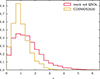 |
Fig. A.1. Redshift distributions of the mock and the COSMOS2020 datasets. For the latter, we consider the photometric redshift calculated with LePhare and available in The Classic catalogue. |
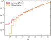 |
Fig. A.2. VISTA H magnitude distributions of the mock and the COSMOS2020 datasets. |
Characteristics of filters in COSMOS2020 used for template fitting.
Principal Component Coefficients for each VISTA HC.
Principal component coefficients for each Euclid-like HC.
All Tables
Forecast red quasars’ completeness (C) and purity (P) from NIR selection functions.
All Figures
|
Fig. 1. Set of passbands describing the photometry of mock red quasars. The panels show the transmission efficiencies for the broad-band optical DECam griz filters, the Euclid VIS (optical) and NISP (NIR) filters, and the NIR to MIR VISTA JHKs filters. The vertical dashed lines are placed at the weighted central wavelength of each filter. |
| In the text | |
|
Fig. 2. Spectrum comparison between unobscured quasar stack (dark blue line; Euclid Collaboration: Lusso et al. 2024) and a reddened quasar spectrum with E(B − V) = 0.25 (light blue line). Emission lines are highlighted using coloured vertical markers along with their respective labels, pointing to different atomic species and ionisation states. The coloured bars correspond to the redshift range of the red grism of NISP. |
| In the text | |
|
Fig. 3. Luminosity-redshift plane for mock sample of red quasars. The black line is the knee of the luminosity function of Glikman et al. (2018). |
| In the text | |
|
Fig. 4. Hyper colour-colour diagram obtained using VISTA+DECam photometry, showing the separation of mock red quasars from COSMOS2020 sources. The latter include galaxies (gold contours) and AGN candidates (in purple). The contours are normalised to their respective subsets. The proposed selection function is displayed via the grey dashed lines. |
| In the text | |
|
Fig. 5. Hyper colour-colour diagram obtained using Euclid-like photometry, showing separation of mock red quasars from COSMOS2020 galaxies (gold contours) and AGN candidates (in purple). The proposed selection function is displayed via the grey dashed lines. |
| In the text | |
|
Fig. 6. VISTA+DECam colour-colour diagram showing separation of mock red quasars from COSMOS2020 galaxies (gold contours) and AGN candidates (in purple). The proposed selection function is displayed by the grey dashed lines. A subset of COSMOS2020 candidate AGNs overlays the selection, colour-coded as i − Ks. |
| In the text | |
|
Fig. 7. VISTA+DECam colour-z diagram showing the separation of mock red quasars from COSMOS2020. The colour-codes adopted for the displayed populations are as in Fig. 6. |
| In the text | |
|
Fig. 8. Euclid-like colour-colour diagram showing separation of mock red quasars from COSMOS2020. The proposed colour-colour selection function is displayed via the grey dashed lines. The COSMOS2020 sample passing the selection is displayed in purple. |
| In the text | |
|
Fig. 9. Euclid-like colour-redshift diagram showing separation of mock red quasars (in red) from COSMOS2020 (golden contours). The COSMOS2020 passing the proposed CC cut is displayed in purple. |
| In the text | |
|
Fig. 10. Colour-colour diagram showing separation of mock red quasars from the Euclid Q1 sample. The proposed colour-colour selection is displayed via the grey dashed lines. The control samples are colour-coded by IE − HE; dots and diamonds represent MIR-selected and radio-selected AGNs, respectively. |
| In the text | |
|
Fig. 11. Colour-z diagram showing separation of mock red quasars from the Euclid Q1 sample. The proposed colour-colour selection is displayed by the grey dashed line. The control samples are colour-coded by IE − HE; dots and diamonds represent the MIR-selected and radio-selected AGNs, respectively. The contours are coloured as in Fig. 10. |
| In the text | |
|
Fig. 12. UMAP visualisation for the results of the probabilistic RF classifier run on the most significant colour features based on PCA. Hexagons are colour-coded by probability of being a candidate red quasar. The overlaid scatter plot displays a random subset with symbols reflecting the empirical CC cut. Stars represent objects previously classified as red quasars. Circles are employed otherwise. |
| In the text | |
|
Fig. 13. UMAP visualisation of Euclid Q1 dataset, colour-coded by the RF-based probability of being a red quasar. The overlaid scatter plot displays 25% of the validation samples. MIR and radio-selected candidate AGNs are marked by circles and diamonds, respectively. The symbols are filled in white if the source passed the empirical CC cut; otherwise, they are coloured in light grey. |
| In the text | |
|
Fig. 14. Candidate red quasars. Panels show, from left to right, the RGB image and the HE, JE, YE, and IE bands. Raw images were obtained through ESA Datalabs (Navarro et al. 2024). |
| In the text | |
|
Fig. 15. Optical-to-NIR colour distributions for EDF-F sample of candidate red quasars observed through both Euclid and VISTA+DECam photometry. The orange and purple distributions are for candidates selected only via Euclid and VISTA+DECam colours, respectively. |
| In the text | |
|
Fig. 16. Examples of two candidate red quasars. The first and the second rows show an Euclid-only and VISTA+DECam-only-selected candidate, respectively. Panels from left to right display the object in the IE and HE filters, in DECam i and VISTA Ks. |
| In the text | |
|
Fig. A.1. Redshift distributions of the mock and the COSMOS2020 datasets. For the latter, we consider the photometric redshift calculated with LePhare and available in The Classic catalogue. |
| In the text | |
|
Fig. A.2. VISTA H magnitude distributions of the mock and the COSMOS2020 datasets. |
| In the text | |
Current usage metrics show cumulative count of Article Views (full-text article views including HTML views, PDF and ePub downloads, according to the available data) and Abstracts Views on Vision4Press platform.
Data correspond to usage on the plateform after 2015. The current usage metrics is available 48-96 hours after online publication and is updated daily on week days.
Initial download of the metrics may take a while.