| Issue |
A&A
Volume 699, July 2025
|
|
|---|---|---|
| Article Number | A318 | |
| Number of page(s) | 12 | |
| Section | Planets, planetary systems, and small bodies | |
| DOI | https://doi.org/10.1051/0004-6361/202554439 | |
| Published online | 16 July 2025 | |
Evaluating the contribution of Tianwen-4 mission to Jupiter’s gravity field estimation using inter-satellite tracking
1
State Key Laboratory of Information Engineering in Surveying, Mapping and Remote Sensing, Wuhan University,
Wuhan,
China
2
Xinjiang Astronomical Observatory, Chinese Academy of Sciences,
Urumqi
830011,
China
3
Geodesy Observatory of Tahiti, University of French Polynesia,
BP 6570, Faa’a, Tahiti
98702,
French Polynesia,
France
★ Corresponding author: jgyan@whu.edu.cn
Received:
9
March
2025
Accepted:
13
June
2025
Context. The upcoming Chinese Tianwen-4 mission, featuring both primary and secondary satellites, promises to significantly enhance our understanding of Jupiter’s gravity field. We provide here a comprehensive evaluation of its contribution to modeling of Jupiter’s gravity field.
Aims. This study investigates the potential contribution of the Tianwen-4 mission to the estimation of Jupiter’s gravity field and the tidal effects knm associated with the Galilean moons by incorporating spacecraft-to-spacecraft tracking (SST) alongside traditional two-way (2W) observations.
Methods. We analyze various observational factors, such as orbital altitudes, noise levels, data durations, and tidal responses, to evaluate their impact on gravity field estimation accuracy.
Results. Our analysis demonstrates that the combined 2W and SST mode enhances the precision of gravity field estimates by up to an order of magnitude, reducing formal errors, and improving spatial resolution compared to the 2W mode alone, even when using shorter arcs data. Furthermore, the combined mode yields a superior performance in the estimation of Love numbers, with lower orbital altitudes and longer data collection periods further improving accuracy, despite introducing operational challenges.
Conclusions. The enhanced sensitivity and accuracy provided by the SST configuration offer valuable insights into Jupiter’s internal structure and dynamics, thereby guiding the design of future missions aimed at maximizing scientific returns.
Key words: gravitation / methods: data analysis / space vehicles / celestial mechanics / planets and satellites: gaseous planets / planets and satellites: individual: Jupiter
© The Authors 2025
 Open Access article, published by EDP Sciences, under the terms of the Creative Commons Attribution License (https://creativecommons.org/licenses/by/4.0), which permits unrestricted use, distribution, and reproduction in any medium, provided the original work is properly cited.
This article is published in open access under the Subscribe to Open model. Subscribe to A&A to support open access publication.
1 Introduction
Jupiter’s gravity field provides unique insights into the planet’s internal structure, composition, and dynamic behavior. Early missions, such as Pioneer 10 and 11 in the 1970s (Null 1976), and Voyager 1 and 2 (Lindal et al. 1981), offered initial insights into Jupiter’s gravity field, while the Galileo orbiter in 1995 revealed a dense core and powerful magnetosphere (D’Amario et al. 1992). The Juno mission, orbiting Jupiter since 2016, has provided precise gravity measurements, allowing scientists to better understand the planet’s interior and study its deep atmosphere and differential rotation (Asmar et al. 2017; Bolton et al. 2021). These findings contribute to our understanding of Jupiter’s formation and the dynamics of gas giants, as well as their role in shaping the Solar System (Stevenson 2020).
Jupiter’s atmosphere is characterized by strong east-west zonal jet streams that contribute to the planet’s distinctive red and white bands (Vasavada & Showman 2005). These jet streams include an eastward super-rotating current near the equator, moving at about 100 m/s, and give way to vortex-dominated dynamics near the poles (Bolton et al. 2021). These atmospheric movements significantly influence Jupiter’s gravitational field by altering the planet’s internal density distribution (Kaspi et al. 2010), which is reflected in its gravity model coefficients (Iess et al. 2018). Early findings from the Juno mission revealed a north-south imbalance in Jupiter’s gravitational field, which corresponds to variations in wind patterns observed at the cloud level (Kaspi et al. 2018). This imbalance aligns with predictions about the gravitational effects of varying flow depths, derived from the study of gravity harmonics (Kaspi 2013).
Jupiter’s gravity field is influenced by both static and dynamic density components. The static component is symmetrical (Guillot 1999), while the dynamic component, driven by atmospheric flows, contributes to both symmetric and asymmetric elements. The impact of these dynamic factors becomes especially prominent in higher-degree gravity harmonics beyond J10, where the gravity signal is predominantly shaped by variations in wind-induced density changes (Kaspi 2013). Additionally, Juno’s precise measurements revealed that Jupiter’s gravity field is affected by internal oscillations or normal modes further complicating its gravitational dynamics (Durante et al. 2022).
Earlier research, including studies by Folkner et al. (2017), Iess et al. (2018), Durante et al. (2020), and Parisi et al. (2021), revealed that gravity measurements from Juno could identify individual harmonics up to J12, allowing scientists to evaluate the depths of Jupiter’s atmospheric flows. This was done by analyzing low-degree odd harmonics (J3, J5, J7, and J9) and isolating the static component from even harmonics (J6–J10) based on models of Jupiter’s internal structure.
Notably, Juno’s precision has shown that the influence of dynamic processes on Jupiter’s gravity field becomes predominant at J10 and marks a critical transition point in the gravity spectrum (Guillot et al. 2018). Recent studies extended the analysis to J40, revealing how Jupiter’s cylindrical atmospheric flows influence gravity harmonics and generate wavy patterns. This advancement through spatial constraints at high latitudes links cloud-level winds to deeper atmospheric structures and underscores the impact of cylindrical flows on Jupiter’s gravity field (Kaspi et al. 2023).
Jupiter’s tidal effects caused by the gravitational pull of its moons are measured using tidal Love numbers (Love 1911), which are essential for understanding the planet’s deep internal structure. Studies by Wahl et al. (2016), Iess et al. (2018), Notaro et al. (2019), and Durante et al. (2020) highlight the importance of these measurements in revealing Jupiter’s internal composition and dynamics. For Tianwen-4, accurate tidal measurements require more regular sampling of Jupiter’s moon longitudes during gravity-focused pericenter passes, enabling a better assessment of the tidal bulge and gravitational interactions.
The formal errors in Jupiter’s gravity field model arise largely due to noise in the observational data and limitations in the spatial resolution of the gravity measurements (Kaspi et al. 2023). At higher degrees, the gravity signal often falls below the noise level and makes it difficult to distinguish the true gravitational variations from observational noise (Kaspi et al. 2023). This is particularly problematic in regions near the poles where most of the Juno spacecraft’s gravity measurements are concentrated, limiting the accuracy of higher-degree harmonics. Additionally, the wavy pattern in the gravity signal caused by interactions with Jupiter’s strong zonal winds further complicates the interpretation of gravity harmonics. As a result, formal errors increase at higher degrees.
An effective way to further mitigate noise issues that affect Earth-based measurements is by using inter-satellite tracking, also known as spacecraft-to-spacecraft tracking (SST), as has been demonstrated by the GRACE and GRAIL missions, and its potential application to Mars (Yan et al. 2024). GRACE produced highly accurate Earth gravity models (Tapley et al. 2005, 2004) and GRACE-FO refined these using laser ranging interferometry (Kornfeld et al. 2019). For the Moon, traditional two-way (2W) doppler tracking resolved the gravity field up to degree 150 (Yan et al. 2020) whereas GRAIL achieved detailed lunar gravity field models up to degree and order 1500 (Park et al. 2015). Leveraging advances from earlier missions (Sun et al. 2025), China’s Tianwen-4 mission is expected to consider SST as a possible technique for investigating the Jupiter gravity field.
This paper evaluates how inter-satellite observations can enhance the accuracy of spherical harmonic coefficients up to degree 40. Using data anticipated from the Tianwen-4 mission, which employs an inter-satellite configuration to study Jupiter, this study proposes a flexible observational strategy. The main spacecraft provides comprehensive gravity measurements and a smaller polar satellite delivers detailed observations, improving insights into Jupiter’s gravity field and internal structure. The paper is organized as follows: Section 2 describes the methodology, including the simulation setup, estimation setup, dynamical models, and solve parameters used. In Section 3, we discuss the results of the simulation and their implications for planetary science. Finally, Section 4 concludes with a summary of the key findings.
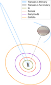 |
Fig. 1 Orbital configuration of Tianwen-4 primary and secondary satellites around Jupiter, including major moons. The graph is on the scale of approximately 6 million kilometers for the X axis, 5.7 million kilometers for the Y axis, and 1.4 million kilometers for the Z axis. |
2 Methodology
Following the success of Tianwen-1 (Sun et al. 2025), Tianwen-4 aims to expand our understanding of the Jovian system. Scheduled for launch in 2029 and arrival at Jupiter by 2035 (Xu et al. 2022). The mission will delve into Jupiter’s atmosphere, magnetosphere, and gravity field, providing invaluable data on the planet’s internal structure, mass distribution, and the mechanisms driving its dynamic weather patterns, including the iconic Great Red Spot (Parisi et al. 2021). Additionally, Tianwen-4 will focus on Jupiter’s Galilean moons, particularly Callisto (Sun et al. 2024). The mission will explore Callisto’s topography, gravity field, and interior structure, providing insights into its geological history.
Figure 1 illustrates the orbital configuration of the Tianwen-4 mission, showcasing the primary and secondary satellites orbiting Jupiter. This figure also highlights the trajectories of Jupiter’s major moons including Io, Europa, Ganymede, and Callisto. This configuration demonstrates the mission’s capability to conduct SST and simultaneous observations of the Jovian system enabling precise gravity field measurements and detailed studies of Jupiter’s environment and its moons.
Scenarios examined in the simulation.
2.1 Description of simulation
In this study, we assess how the Tianwen-4 mission’s observation data could impact the accuracy of Jupiter’s gravity field estimation by focusing on the performance of the inter-satellite configuration used in our simulations. The study includes two satellite orbits: a primary spacecraft following the proposed trajectory of the Tianwen-4 mission with an inclination of 40° (Afzal et al. 2025), chosen to facilitate the study of Jupiter’s magnetosphere. Simultaneously, the secondary satellite placed in a Jovian polar orbit will complement these measurements by focusing on the gravity field in the high-latitude regions where Jupiter’s complex magnetic and gravitational interactions are most pronounced.
By combining data from both the highly eccentric and circular polar orbits the mission aims to construct a highly detailed, spherical model of Jupiter’s gravity field. In the context of this study, we define two observation modes: the native “2W mode” whereby only the primary spacecraft is tracked via a 2W Doppler from Earth, and the “combined mode” which incorporates both 2W ground tracking of the primary and inter-satellite tracking between the two spacecraft. We have outlined and analyzed four scenarios which are detailed in Table 1.
Table 1 presents the simulation scenarios examined in this study based on the initial orbital elements of the Tianwen-4 mission. These scenarios systematically vary four key parameters to assess their impact on Jupiter’s gravity field estimation. The observation modes include 2W tracking and a combined mode. The secondary spacecraft is placed at different orbital altitudes, 3500 km, 4500 km, and 5500 km to evaluate how intersatellite distance affects measurement sensitivity. SST observation noise levels are varied across three orders of magnitude, from 1 mm/s, 0.1 mm/s, and 0.01 mm/s, to simulate different levels of instrument precision. Mission durations range from 6 months to 2 years allowing the analysis to capture how extended mission time contributes to improved quality. This configuration enables a detailed evaluation of SST’s role in enhancing spatial resolution and reducing uncertainties. The analysis includes gravity field coefficients, parameter intercorrelations, orbit determination accuracy, tidal Love numbers, and error distributions. Results based on these scenarios are presented in Section 3 and further elaborated in the subsequent sections.
For the Tianwen-4 primary spacecraft 2W satellite tracking is conducted using terrestrial stations from the Chinese Deep Space Network (CDSN), specifically in Kashi (China), Jiamusi (China), and Neuquén (Argentina) (Dong et al. 2017). In our analysis, we utilized two visibility configurations. For the primary spacecraft, we set the ground station elevation angle to a minimum of 10 degrees. Additionally, for both the primary and secondary spacecrafts, we accounted for Jupiter as an occultation body by considering times when the planet blocks the line of sight between both spacecrafts and spacecraft to Earth.
To investigate the potential contributions of radio tracking data from both the native 2W only and combined mode configurations in studying Jupiter’s gravity field, we conducted numerical simulations using the TU Delft Astrodynamics Toolbox (Tudat)1,2 (Dirkx et al. 2019, 2022). Tudat has a strong track record of being employed for both simulated and real analyzes of radio science solutions in planetary missions (Bauer et al. 2016; Fayolle et al. 2023, 2024).
To accurately model the trajectories of both primary and secondary satellites for the combined mode, we propagated their arcs over 3.35-hour intervals centered on each perijove to minimizing integrator error accumulation and enhancing parallel computational efficiency. For the 2W alone mode, a 10-hour arc was used to maintain consistency and optimize simulation accuracy. We simulated datasets for different durations that begin in April 2037. For both spacecraft, we also accounted for the northward shift in orbital parameters induced by gravitational effects after each orbit. A 60-second integration time step was used for all cases listed in Table 1 during this simulation experiment to ensure sufficient sampling of the gravitational signal.
Furthermore, we excluded ground station overlaps between observations. The combined mode observations were only considered when the primary satellites reached their closest approach to the periapsis and the distance between the two satellites was less than 250 000 km, similar to China’s DRO mission, which used high inter-satellite distances to optimize tracking (Li et al. 2022).
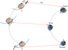 |
Fig. 2 Schematic diagram of the SST and 2W observation modes. |
2.2 Inter-satellite observation mode
Two observation modes were developed, as is illustrated in Figure 2. The red lines indicates the 2W range-rate measurement between the ground station on Earth and the primary satellite orbiting Jupiter, referred to as 2W. The black line represents the range-rate measurement between the primary and secondary satellites, known as SST.
A simplified measurement equation for the SST observation (Yao et al. 2021), developed for GRAIL observations, is as follows:
![$\[\dot{\rho}(t)=\frac{\left[\boldsymbol{r}_p\left(t-\Delta t_p\right)-\boldsymbol{r}_s(t)\right] \cdot\left[\dot{\boldsymbol{r}}_p\left(t-\Delta t_p\right)-\dot{\boldsymbol{r}}_s(t)\right]}{\left|\boldsymbol{r}_p\left(t-\Delta t_p\right)-\boldsymbol{r}_s(t)\right|}+\epsilon.\]$](/articles/aa/full_html/2025/07/aa54439-25/aa54439-25-eq1.png) (1)
(1)
In this equation, rp(t − Δtp) represents the position vector of the primary satellite within the barycentric celestial reference system and rs(t) denotes the position vector of the secondary satellite in the same system. Δtp is the light-time delay from the secondary satellite to the primary satellite. t represents the time instance at which the signal is either transmitted or received. The vector rp(t − Δtp) − rs(t) defines the relative position of the primary satellite with respect to the secondary satellite while ![$\[\dot{\boldsymbol{r}}_{p}\left(t-\Delta t_{p}\right)-\dot{\boldsymbol{r}}_{s}(t)\]$](/articles/aa/full_html/2025/07/aa54439-25/aa54439-25-eq2.png) indicates the relative velocity between the two satellites, and ε represents an error term. This relative velocity represents the range-rate data between the primary and secondary satellites. An in-depth analysis of the SST technology used in the GRAIL mission is provided by Genova & Petricca (2021).
indicates the relative velocity between the two satellites, and ε represents an error term. This relative velocity represents the range-rate data between the primary and secondary satellites. An in-depth analysis of the SST technology used in the GRAIL mission is provided by Genova & Petricca (2021).
Nevertheless, here we are using Eq. (1) in a vastly different context compared to the GRAIL experiment, as the mass of Jupiter is 25 900 times the mass of the Moon, and the separation between the two spacecraft can reach approximately 250 000 km, instead of 217 km for GRAIL (see Figure 3). Therefore, Eq. (1) should, in principle, be corrected for the bending of space-time caused by Jupiter (ε error term in Eq. (1)) to be coherent with the relativistic acceleration mentioned later in Section 2.4.3 (Schwarzschild radius of Jupiter). In this simulation, we chose to apply Eq. (1) as it is to avoid unnecessary complexity, as this effect is very small.
Figure 3 shows the time delay in signal transmission from the primary satellite to the secondary satellite, accounting for varying distances and orbital dynamics. Each line represents the delay for an individual arc spanning from the start time to the end time. The figure combines data from all 36 arcs to illustrate the overall variation in signal delay between the two satellites.
To ensure a precise time lag for the measurements (Casini et al. 2023) clock synchronization between Earth and both satellites was achieved by estimating and correcting the clock biases using ranging signals from Earth. However, for simplification in this simulation we assumed that the time tagging of all the measurements was accurate, as taking into account time tag errors would introduce additional complexity without significantly affecting the overall results (Müller et al. 2022).
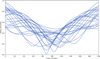 |
Fig. 3 Light-time delay (Δtp) variation between the primary and secondary satellites across all arcs. Each curve represents the signal transmission delay for a single arc, accounting for variations in distance. |
2.3 Error budget
To make our simulations as realistic as possible the noise budget applied to the 2W data was developed by accounting for error sources commonly encountered in deep-space tracking missions. These include delays caused by signal propagation through the interplanetary plasma, troposphere, and ionosphere; instrumentation-related delays; timing instabilities; signal-to-noise constraints of both the spacecraft and calibrator signals; and uncertainties in ground station locations and Earth orientation parameters (Asmar et al. 2017).
Among these noise sources, phase scintillation plays a particularly important role due to its impact on the signal’s phase stability over time. Caused by propagation through turbulent plasma and atmospheric layers, scintillation introduces temporally correlated noise that can significantly degrade Doppler tracking accuracy particularly at X- and Ka-band frequencies. Tropospheric scintillation typically peaks at 2W light time, while plasma-induced fluctuations dominate the low-frequency noise spectrum (Armstrong 1998). Accurately modeling these effects is essential for achieving high-precision orbit determination and gravity field recovery.
Although the original Tianwen-4 mission design includes dual-frequency (X and Ka band) 2W tracking to correct for dispersive media effects, our simulations considered only single-frequency 2W Doppler observables which were deemed sufficient for the intended analysis. As we used a statistical approach we applied Gaussian white noise with a standard deviation of 0.05 mm/s to the primary satellite observations, consistent across all cases.
Jupiter is surrounded by a strong and extensive magnetosphere which contains dense and highly energetic plasma (Connerney et al. 2017). This environment can introduce frequency-dependent propagation effects such as group delay and phase scintillation into SST observations due to interactions with charged particles (Xu et al. 2024). Although modeling these effects is beyond the scope of this study they represent a critical source of potential error and should be investigated in detail in future work. For the purpose of simulation we tested three different noise levels: 1 mm/s, 0.1 mm/s, and 0.01 mm/s, as is discussed in Section 2.1.
2.4 Estimation methodology
2.4.1 Covariance analysis
The covariance matrix, P, of the estimated parameters was determined using the following Gaussian approach (Montenbruck & Gill 2002):
![$\[P=\left(H^T W H+P_0^{-1}\right)^{-1}.\]$](/articles/aa/full_html/2025/07/aa54439-25/aa54439-25-eq3.png) (2)
(2)
In Eq. (2), W represents the sum of observation and model errors weight matrix (Barriot & Balmino 1992) while H is the partial derivative matrix of the observations with respect to the estimated parameters. The matrix P0 contains the a priori covariances of the estimated parameters reflecting our initial knowledge before the estimation process. The accuracy of the estimation is then statistically represented by the covariance matrix Pc, which is defined as follows:
![$\[P_c=P+\left(P H^T W\right)\left(H_c C H_c^T\right)\left(P H^T W\right)^T.\]$](/articles/aa/full_html/2025/07/aa54439-25/aa54439-25-eq4.png) (3)
(3)
The matrices P, H, and W refer to the same matrices that are described in Eq. (2). Here, Hc represents the observation partial derivatives concerning the considered parameters and C is the covariance matrix that reflects our knowledge of these considered parameters. The formal uncertainties of the estimated parameters were calculated as the square root of the diagonal elements of P and Pc. The propagated covariance was obtained using the following method:
![$\[P(t)=\left[\begin{array}{ll}\Phi\left(t, t_0\right) & S(t)\end{array}\right] P\left[\begin{array}{ll}\Phi\left(t, t_0\right) & S(t)\end{array}\right]^T.\]$](/articles/aa/full_html/2025/07/aa54439-25/aa54439-25-eq5.png) (4)
(4)
In Eq. (4), Φ(t, t0) represents the state transition matrix and S(t) denotes the sensitivity matrix. The same equation can be used to propagate the considered covariance matrix Pc instead of P. While covariance analyzes are well suited for our purposes they are based on several simplifying assumptions. In our approach Doppler data from each observation arc of both spacecraft are incorporated into a multi-arc and multi-body framework, with Jupiter’s orbit being modeled continuously for the entire mission duration. This setup allows the data from each arc to contribute to global parameters, such as Jupiter’s gravity field, tidal responses, and the planet’s position and velocity, as well as local parameters specific to each arc, including the position and velocity of both spacecraft. Additionally, Doppler measurements are calculated by solving the relativistic light-time equation with Jupiter’s oblateness accounted for in the spacecraft’s orbital modeling. However, the formal uncertainties derived from this process always provide an optimistic statistical representation.
2.4.2 Theoretical framework
The primary factor contributing to the spacecraft’s acceleration is Jupiter’s static gravitational field, which can be described by the following potential (Bertotti et al. 2003):
![$\[\begin{aligned}U(r, \theta, \phi)= & \frac{G M}{r} \sum_{n=0}^{\infty} \sum_{m=0}^n\left(\frac{R_e}{r}\right)^n P_{n, m}(\sin \theta) \\& {\left[C_{n, m} \cos (m \phi)+S_{n, m} \sin (m \phi)\right] }\end{aligned}.\]$](/articles/aa/full_html/2025/07/aa54439-25/aa54439-25-eq6.png) (5)
(5)
In Eq. (5), G represents the universal gravitational constant, M is the mass of Jupiter and Re is the reference equatorial radius of Jupiter (71 492 km). The terms Pn,m are the associated Legendre functions, while Cn,m and Sn,m are the unnormalized spherical harmonic coefficients. The gravitational acceleration experienced by an external point source such as the spacecraft is determined by the gradient of this gravitational potential and is defined by the latitude (θ), longitude (ϕ), and radius (r) of the point source.
Jupiter’s static gravity field is predominantly axially symmetric and it is typically described using zonal parameters Jn = −Cn,0. However, our model also accounts for the quadrupole gravitational harmonics C2,1, S2,1, C2,2, and S2,2, which are determined by Jupiter’s inertia tensor and reflect the planet’s deviation from axial symmetry due to its internal mass distribution and rotation. Although for Jupiter, these values are expected to be close to zero with upper limits constrained by Juno’s observations (≲10−9), we included them in our model. All other static tesseral coefficients (where m ≠ 0) were set to zero.
In addition to a static background, Jupiter’s gravity field is influenced by dynamic factors that change over time (Love 1911). The tidal forces exerted by the Galilean moons create significant bulges on the planet which in turn modify its gravitational field. To account for these dynamic effects, we incorporated variations in the gravitational parameters using the following equations:
![$\[\begin{aligned}&\Delta \bar{J}_n=\frac{-1}{2 n+1} k_{n 0} \sum_j \frac{G M_j}{G M_{\oplus}}\left(\frac{R}{r_j}\right)^{n+1} \bar{P}_{n 0}\left(u_j\right),\\&\Delta \bar{C}_{n m}-i \Delta \bar{S}_{n m}= \frac{1}{2 n+1} k_{n m} \sum_j \frac{G M_j}{G M_{\oplus}}\left(\frac{R}{r_j}\right)^{n+1} \bar{P}_{n m}\left(u_j\right) \\&\qquad\qquad\qquad\qquad\left(s_j-i t_j\right)^m.\end{aligned}\]$](/articles/aa/full_html/2025/07/aa54439-25/aa54439-25-eq7.png) (6)
(6)
In Eq. (6), ![$\[\bar{C}_{n, m}\]$](/articles/aa/full_html/2025/07/aa54439-25/aa54439-25-eq8.png) and
and ![$\[\bar{S}_{n, m}\]$](/articles/aa/full_html/2025/07/aa54439-25/aa54439-25-eq9.png) are the fully normalized spherical harmonic coefficients corresponding to the degree n and order m. The term GM⊕ represents Jupiter’s gravitational parameter while GMj refers to the gravitational parameter of the jth moon. The variable rj indicates the radial distance from Jupiter to the jth moon. Additionally, sj, tj, and uj are the Cartesian components of the unit vector fixed within Jupiter’s body frame, pointing toward the jth perturbing moon.
are the fully normalized spherical harmonic coefficients corresponding to the degree n and order m. The term GM⊕ represents Jupiter’s gravitational parameter while GMj refers to the gravitational parameter of the jth moon. The variable rj indicates the radial distance from Jupiter to the jth moon. Additionally, sj, tj, and uj are the Cartesian components of the unit vector fixed within Jupiter’s body frame, pointing toward the jth perturbing moon.
To model the oscillations observed in Juno Doppler residuals and attributed to normal modes by Durante et al. (2022), we incorporated empirical accelerations into our gravitational model using the following equation (Montenbruck & Gill 2002):
![$\[a=R^{I / R S ~W}\left(a_0+a_1 ~\sin~ v+a_2 ~\cos~ v\right).\]$](/articles/aa/full_html/2025/07/aa54439-25/aa54439-25-eq10.png) (7)
(7)
Eq. (7) represents acceleration in the RS W frame where RI/RS W is the rotation matrix to the inertial frame, a0 is a constant bias and a1, a2 are one-cycle-per-revolution (1CPR) coefficients. The terms sin v and cos v with v as the true anomaly represent periodic mismodeling at 1CPR. This approach incorporates empirical accelerations to model unexplained forces affecting spacecraft motion, providing flexibility to align simulations with observed data without requiring a detailed physical model of Jupiter’s normal modes.
2.4.3 Dynamical models
The dynamical models for both spacecraft incorporate several key effects that significantly influence their motion around Jupiter. The overall modeling approach is similar to that of Afzal et al. (2025). These models include:
Gravitational accelerations, which are considered within a framework accounting for their relative motion.
The gravitational influence of point masses, including the planets in the Solar System and Jupiter’s Galilean moons.
Jupiter’s oblate gravitational field, modeled using spherical harmonics.
Gravitational variations due to solid body tides caused by the Jovian moons.
Jupiter’s rotation, which is considered at a reference epoch within the IAU-defined reference frame.
Changes in Jupiter’s spin axis orientation.
Relativistic perturbation (Schwarzschild radius of Jupiter).
The synchronous rotation of Jupiter’s moons.
Solar radiation pressure, accounted for using a simplified cannonball model.
Empirical accelerations.
For planetary and satellite ephemerides, we used JPL’s DE4403 and JUP3654 (Park et al. 2021). The dynamical models account for Jupiter’s gravity field up to degree 40 (covering coefficients from J40 to J2) including the tesseral coefficients C2,1, C2,2, S2,1, and S2,2. The baseline values for these gravity field coefficients are based on the most recent solution by Kaspi et al. (2023).
Furthermore, for the Tianwen-4 primary spacecraft empirical accelerations were considered during each flyby within specific 2-hour windows with a period of 12 minutes. In contrast, for the secondary spacecraft empirical accelerations were accounted for continuously throughout its entire orbit as it follows a nearly circular trajectory and the spacecraft experiences empirical accelerations along its entire path.
These accelerations can present themselves differently on the two spacecraft because of their distinct orbital configurations of primary and secondary orbit although they arise from the same physical source, namely the normal modes of Jupiter. The effect of empirical acceleration is simulated in the same way but not correlated for both spacecraft as we have no other way to model it.
Parameter details and constraints for Jupiter and Tianwen-4.
2.5 Explanation of the solve-for parameters
The parameters estimated from the simulated radio-science observations are presented in Table 2. We differentiate between the global and local state estimation setups. A key enhancement of our baseline setup compared to most radio-science solutions is the inclusion of Jupiter’s state estimation alongside the spacecraft’s orbits. This approach is designed to enhance the robustness of gravity field estimation.
Additionally, we included the Love numbers k22, k31, k33, k42, and k44 in our model. Specifically, k22 was estimated individually for each of Jupiter’s Galilean moons, while the combined effect of all moons was considered for k31, k33, k42, and k44. This approach was selected to strike a balance between obtaining detailed information on tidal responses and avoiding overparameterization ensuring the statistical stability of the model.
By estimating k22 separately for each moon, we aimed to capture their individual tidal responses. Meanwhile, estimating the higher-order Love numbers collectively allowed us to evaluate overall tidal effects without risking instability in the model. The values of knm with odd n − m are not observable due to the slight inclination of Jupiter’s satellite orbits. The values for kn0 were fixed according to model predictions as they are not observable due to their high correlation with the Jn coefficients (Durante et al. 2020). Additionally, the same Love number was assumed for all the Galilean moons Io, Europa, Ganymede, and Callisto.
In this study, constraints were applied selectively to the gravity field coefficients. In the case of 2W mode, the first 12 coefficients (J2 to J12) were left unconstrained as they are well resolved by the data. Higher-degree harmonics (J13 to J40) more sensitive to noise, were constrained using the formal uncertainty values of Kaspi et al. (2023), who applied a Kaula-type constrained gravity solution using special constraints to stabilize the estimation of high-degree harmonics. However, this constraint was loosened to allow for a broader evaluation of uncertainties. In contrast, for the combined mode, no constraints were applied as the data provided sufficient resolution for us to determine the gravity field coefficients across all degrees.
3 Results
The accuracy of Jupiter zonal harmonic coefficients and tidal Love number knm was assessed using formal error analysis. By leveraging SST data and varying observational configurations the results provide insights into the precision achievable under different scenarios. This section details the impact of key factors such as orbital altitude, noise levels, and mission duration on the reliability of the gravity field estimation and the estimation of tidal Love numbers.
3.1 Gravity field estimation
The labels in Figures 5 through 11 represent different models used to analyze the formal errors of Jupiter’s gravity field. Each model is derived from various data sources and methodologies. The “Reference Model” refers to the established gravity field of Jupiter resolved by Kaspi et al. (2023) and serves as a benchmark for comparing other models. By incorporating different scenarios outlined in Table 1 applied within the SST mode, we aim to enhance accuracy and improve our understanding of Jupiter’s gravity field. The reference values of the Jn coefficients based on Kaspi et al. (2023) are plotted in Figure 4.
Figure 4 presents the Jn values of the reference model. Due to the significant differences between the first 9 coefficients and the higher-degree values, the axis is split into two parts: the left axis represents the first 9 Jn zonal harmonics with a scale set to 10−3, while the right axis plots the remaining Jn values (10 to 40) with a scale set to 10−7.
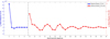 |
Fig. 4 Reference model zonal harmonics (Jn) used in the simulation. The plot is split into two axes to accommodate scale differences: the left axis shows the first 9 Jn coefficients scaled to 10−3, while the right axis displays degrees 10 to 40 scaled to 10−7. |
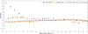 |
Fig. 5 Formal uncertainties (σ) of gravity field coefficients from the 2W mode at 40° and 90° orbital inclinations, alongside the reference model. Red and blue squares denote the positive and negative values of the reference Jn coefficients, respectively. The 40° inclination results in higher uncertainties due to limited latitudinal coverage, especially at low degrees. In contrast, the 90° polar orbit significantly reduces formal errors across all degrees, emphasizing the importance of comprehensive latitude coverage in achieving accurate gravity field recovery. |
3.1.1 Effects of observation modes
Figures 5 and 6 illustrate the formal errors resulting from the native 2W mode as well as the formal errors from combined mode. Additionally, the figures include the formal errors of the reference model derived by Kaspi et al. (2023) and the reference values of the Jn coefficients, providing a comparative baseline for evaluating the accuracy of the estimated gravity field. The figures highlights how the fusion of these data sources enhances the accuracy of the estimated gravity field model of Jupiter. By comparing the formal errors from the combined mode with those from the 2W mode alone, we can evaluate the effectiveness of this combined approach in improving the precision of the gravity field estimation.
Figure 5 presents the formal uncertainties (σ) of the reference model and the native 2W mode under two different orbital inclinations: 40° and 90°. The corresponding Jn values are also shown using red and blue squares where red indicates positive values and blue indicates negative values of Jn. In the case of the 2W mode with a 40° orbital inclination, the formal uncertainties are larger than those of the reference model up to degree 12. Beyond this point, they slightly decrease and align with the reference model up to degree 40, primarily because the solution is fully constrained by the a priori constraints indicating that the native 2W mode lacks sensitivity to these higher degrees. These larger formal errors are primarily due to the limited latitudinal coverage at 40° inclination which reduces sensitivity to Jupiter’s gravity field variations, particularly near the poles. This incomplete coverage results in less accurate gravity field estimations and inconsistencies with the reference Juno model.
To further confirm the coverage effect the orbital inclination was adjusted to 90°. The Tianwen-4 mission with its 90° inclination provides comparable accuracy to the Juno reference model, whose gravity passes are also captured at around a 90° inclination. However, differences in specific observation modes and data processing techniques lead to variations in formal uncertainties. In contrast a 90° inclination provides much lower uncertainties across both lower and higher degrees because the polar orbit offers comprehensive coverage over all latitudes, including the polar regions. This extensive coverage enhances sensitivity to both large-scale (lower-degree) and fine-scale (higher-degree) gravitational variations, leading to a more reliable and accurate gravity field model as is demonstrated in Afzal et al. (2025). Please note that the native 2W mode with 90° inclination is used solely to validate the coverage aspect while in the rest of the analysis the native 2W mode corresponds to the 40° orbital inclination.
Figure 6 presents the formal uncertainties (σ) for the reference model along with the combined mode with and without empirical acceleration. When the 2W and SST modes are combined the formal uncertainties are significantly reduced, resulting in much smaller formal errors. This improvement is due to the additional tracking data provided by SST, which enhances triangulation and reduces position and velocity errors, particularly at higher degrees where more detailed gravity field features require greater accuracy. Notably, the first 6 degrees exhibit larger formal errors, which then gradually decrease up to degree 12 primarily due to the influence of the empirical acceleration applied in the analysis.
The results without empirical acceleration confirm that its primary influence lies within the first 12 degrees where unmodeled low-frequency forces, such as the ones related to Jupiter’s normal modes, are more prominent. Although empirical accelerations help absorb these effects including them in the estimation increases the number of free parameters, which may introduce strong correlations with low-degree gravity terms. This can inflate the formal uncertainties. At higher degrees where localized gravity signals dominate, these forces become less significant and the empirical terms have a negligible effect, resulting in similar formal errors with or without their inclusion. As is detailed in Section 2.5, no a priori constraints are applied in the combined mode, highlighting that the observed improvements entirely come from the data. Figures 7 and 8 further illustrate this behavior by comparing the correlation structures of the estimation.
Figure 7 presents the correlation matrix derived exclusively from the 2W mode. In this matrix, notable off-diagonal cross-correlations are observed among various parameters including the individual k22 and combined k31, k33, k42, and k44 Love numbers, as well as gravitational coefficients such as C2,0, C2,1, C2,2, and C3,0 through C40,0, along with S2,1 and S2,2. These correlations suggest potential dependencies among the parameters which could complicate the interpretation and accuracy of the gravitational data. Beyond 12 degrees the overall correlation decreases, indicating a reduction in parameter interdependence.
Figure 8 illustrates the correlation matrix obtained from the combined mode. While Figure 7 showed significant off-diagonal correlations the combined mode in this analysis demonstrates a notable reduction in these correlations across most degrees, though some minor dependencies between parameters may still remain. This reduction indicates that the inclusion of SST data helps to minimize the interdependencies among parameters, thereby enhancing the overall accuracy and reliability of the gravitational data. The decrease in correlation suggests that combining 2W and SST mode helps resolve the issues caused by parameter interdependencies in the 2W mode alone leading to a more robust and interpretable gravity field model.
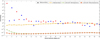 |
Fig. 6 Formal uncertainties (σ of gravity field coefficients for the combined 2W and SST mode is shown with and without empirical acceleration, alongside the reference model. Red and blue squares denote the positive and negative values of the reference Jn coefficients, respectively. The inclusion of empirical accelerations improves alignment with low-degree gravitational signals influenced by empirical acceleration but increases formal errors due to parameter correlations. At higher degrees, where localized gravity dominates, the impact of empirical acceleration diminishes. No a priori constraints are applied, emphasizing that improvements stem entirely from the data. |
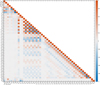 |
Fig. 7 Correlation matrix of estimated parameters from the 2W mode, highlighting significant off-diagonal correlations among tidal Love numbers (k22, k31, k33, k42, k44) and gravity field coefficients (C2,0 to C40,0, C2,1, C2,2, S2,1, and S2,2). The correlations reflect parameter interdependence that may affect estimation robustness. A notable decrease in correlation is observed beyond degree 12, suggesting improved parameter separability at higher degrees. |
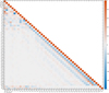 |
Fig. 8 Correlation matrix of estimated parameters from the combined 2W and SST mode, highlighting a significantly reduced off-diagonal correlation among tidal Love numbers k22, k31, k33, k42, k44) and low-degree gravity field coefficients (C2,0 to C40,0, C2,1, C2,2, S2,1, and S2,2). This demonstrates the combined mode’s ability to reduce parameter interdependencies and improve the robustness and interpretability of the gravity field estimation. |
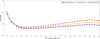 |
Fig. 9 Formal uncertainties (σ) of gravity field coefficients derived from the combined 2W and SST mode at three secondary spacecraft altitudes: 3500 km, 4500 km, and 5500 km. Lower altitudes yield smaller uncertainties, especially beyond degree 12, due to improved sensitivity to short-wavelength gravitational features. |
3.1.2 Effects of orbital altitudes
The orbital altitude around Jupiter is a prime factor in determining the resolution and accuracy of gravity field measurements. A low orbital altitude increases precision as the spacecraft is closer to the gravitational signal source. However, operating at lower altitudes presents challenges including increased exposure to Jupiter’s intense radiation belts and atmospheric effects. Strong zonal winds especially at cloud level raise spacecraft perturbations. Additionally, lower orbits may reduce the spacecraft’s lifetime due to higher atmospheric drag particularly near perijove. Balancing these factors requires one to consider various orbital altitudes to optimize scientific return while ensuring the spacecraft’s longevity and safety. The three different orbital altitudes, 3500 km, 4500 km, and 5500 km, of the secondary satellite, were evaluated using the combined mode as is presented in Figure 9.
Figure 9 illustrates the impact of orbital altitude variations on gravity field estimation by comparing altitudes of 3500 km, 4500 km, and 5500 km. The 3500 km orbit shows the smallest uncertainties (σ) indicating the highest accuracy in gravity field estimation, while errors increase with altitude with 5500 km having the largest uncertainties. Up to degree 12, the formal errors remain relatively consistent across different altitudes as these lower-degree harmonics represent large-scale, long-wavelength features that are detectable even from higher altitudes. Beyond degree 12, a noticeable decrease in formal errors occurs with decreasing altitude since higher-degree harmonics correspond to smaller-scale, short-wavelength structures. These finer details are more sensitive to altitude and being closer to the planet enhances the spacecraft’s ability to resolve them, resulting in more accurate and precise gravity field recovery at lower altitudes.
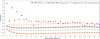 |
Fig. 10 Formal uncertainties (σ) of gravity field coefficients derived from combined 2W and SST mode under varying SST mode noise levels, 1, 0.1, and 0.01 mm/s, while the 2W mode remains fixed at 0.05 mm/s. Red and blue squares denote the positive and negative values of the reference Jn coefficients, respectively. Lower SST noise significantly reduces formal errors, improving sensitivity to both large-scale and fine-scale gravitational features. |
3.1.3 Observation noise levels
Figure 10 illustrates the effect of different noise levels (1, 0.1, and 0.01 mm over a 60 s Doppler window) on the formal errors in the gravity field estimation. For the following results, we consider only the data errors as it is nearly impossible to assess the modeling errors that are probably at the same level. The noise levels are varied only for the SST mode, while the 2W mode maintains the same noise level 0.05 mm/s, remaining unchanged across all the presented cases. This comparison highlights the sensitivity of the SST mode to noise variations while the 2W mode remains more stable under these conditions. It shows that the lowest formal errors are achieved at the noise level of 0.01 mm/s, indicating the highest accuracy in the gravity field estimation. As the noise level increases to 0.1 mm/s and 1 mm/s the formal errors also increase, but they follow a consistent pattern across the degrees. This highlights the sensitivity of the gravity field estimation to varying noise levels as lower noise reduces random errors and enhances the detection of both large- and fine-scale gravitational features, leading to more precise results.
3.1.4 Observation duration
Gravity field accuracy and spatial resolution are strongly influenced by orbital geometry and mission duration. To assess the mission duration’s impact on gravity field estimations Figure 11 illustrates gravity field accuracy variations, while Figure 12 shows corresponding spacecraft ground tracks.
Figure 11 illustrates the effect of mission duration on gravity field estimation by comparing results from 6-month, 1-year, 1.5-year, and 2-year durations. The figure shows that as mission duration increases there is only a minor reduction in formal uncertainties with the two-year duration showing the lowest uncertainties. This is because the longer observation period allows for better averaging of random noise and temporal variations but after a certain point most critical data has already been captured, leading to diminishing returns. Despite differences in uncertainty levels the uncertainties associated with the different mission durations are consistent with each other across all degrees. Longer observations enhance the detection of both long-wavelength and short-wavelength features, thereby reducing uncertainty throughout the spectrum.
Figure 12 presents the ground track coverage for different mission durations of combined mode with panel a representing a 6-month period, panel b showing a 1-year period, panel c illustrating a 1.5-year period, and panel d depicting a 2-year period. The figure demonstrates that as the mission duration increases the ground track coverage becomes more complete. The 6-month period in panel a shows the least coverage while the 2-year period in panel d provides the most extensive coverage. The tracks plotted in red correspond to the primary satellite while the blue tracks represent the secondary satellite. This increased coverage with longer mission durations contributes to a more stable gravity field estimation though the reduction in formal uncertainties is minor as most critical data is captured within the first year.
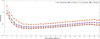 |
Fig. 11 Formal uncertainties (σ) of gravity field coefficients derived from combined 2W and SST mode for mission durations of 6-month, 1-year, 1.5-year, and 2-year periods. Longer durations lead to modest reductions in uncertainties, with diminishing returns beyond the first year. Across all cases, uncertainty patterns remain consistent across degrees. |
3.2 Jupiter tidal estimation
The tidal effects on Jupiter were evaluated using moon-specific estimates of the Love number k22 along with combined estimates for the higher-order Love numbers, as is detailed in the solved parameter section. For the comparison, the reference formal error values for k22 (Io) and the higher-order Love numbers are derived from Durante et al. (2020) which is based on real data. However, since Durante et al. (2020) does not provide moonspecific values for k22 for Europa, Ganymede, and Callisto we have instead referenced the simulation-based values from Notaro et al. (2019). The estimated and reference model uncertainties for these tidal parameters are summarized in Table 3.
Table 3 summarizes the estimated Love numbers and their uncertainties for Jupiter comparing results obtained using the 2W mode, the combined mode, and the reference Juno model. This table provides both individual estimates for each Galilean moon (Io, Europa, Ganymede, and Callisto) and combined estimates for higher-order Love numbers (k31, k33, k42, and k44).
The analysis reveals that for all moons, the 3 σ uncertainty in k22 is lower with the combined mode and the true Juno model even though the observation arcs are shorter at 3.35 hours. This reduction in uncertainty is likely due to the higher spatial resolution provided by the SST mode which is more sensitive to localized gravitational variations and can effectively capture rapid, short-term changes in the moons’ tidal responses. Additionally, the true Juno model serves as a valuable benchmark for comparison highlighting the increased precision achieved through the combined mode.
The combined estimation of higher-order Love numbers (k31, k33, k42, and k44) similarly demonstrates that the combined mode outperforms the 2W mode alone. This is due to the SST’s capability to capture high-frequency gravitational field variations offering an enhanced sensitivity to localized changes that complement the 2W mode’s measurements. Additionally, the combined mode benefits from the complementary geometry of the 2W and SST configurations. This makes the combined approach particularly effective in capturing both short-term gravitational fluctuations and larger-scale gravitational field characteristics leading to improved accuracy in formal uncertainties. Furthermore, the improved accuracy in the 2W observation mode, compared to the reference model is attributed to the higher number of arcs used. We also present the moons’ orbital trajectories during the observation period in Figure 13.
Figure 13 presents the orbital trajectories of Jupiter’s major moons Io, Europa, Ganymede, and Callisto, plotted in polar coordinates. The figure compares the observed moon orbits during the designated observation period for both the 2W mode alone and the combined mode. Panel a shows the 2W mode with a 10-hour observation duration per arc while panel b illustrates the combined mode with a shorter observation duration of 3.35 hours per arc. This visualization highlights the spatial coverage and dynamic motion of the moons as well as the impact of observation duration.
In conclusion, the combined mode consistently delivers better results compared to the 2W-only mode despite the shorter observation arcs of 3.35 hours. The combined mode achieves lower uncertainties and higher precision in estimating the Love numbers of Jupiter’s moons. This improvement is primarily due to the SST mode’s ability to capture localized gravitational variations and high-frequency changes complementing the 2W mode’s broader measurements. The combined approach proves to be more effective in providing detailed and accurate gravitational data as is demonstrated in the analysis of k22, k31, k33, k42, and k44, across different moons.
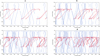 |
Fig. 12 Ground track coverage for different mission durations using the combined 2W and SST mode. (a) 6-month, (b) 1-year, (c) 1.5-year, and (d) 2-year periods. Red and blue tracks represent the ground tracks of the primary and secondary spacecraft, respectively. An increased mission duration leads to more complete coverage. |
Love numbers k22 (satellite-dependent), k31, k33, k42, and k44 (combined effect of all Galilean moons) with 3 σ formal errors for the 2W mode, combined mode, and reference Juno model.
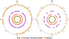 |
Fig. 13 Orbital trajectories of Jupiter’s major moons (Io, Europa, Ganymede, and Callisto) in polar coordinates. Panel a represents a 10-hour observation period during the 2W, while Panel b focuses on a 3.35-hour observation period during the combined 2W and SST mode. |
4 Discussion and conclusion
This study evaluates the potential contribution of the Tianwen-4 mission’s combined 2W and SST mode to the estimation of Jupiter’s gravity field. The results of the simulations are very optimistic, as we used simplifying assumptions. We estimate that, by taking into account these simplifying assumptions (model errors), the combined use of 2W and SST mode improves the accuracy of gravity field estimation by approximately an order of magnitude compared to the reference model. The combined mode in particular shows substantial improvements in reducing formal errors and improving spatial resolution, particularly at higher degrees compared to using the 2W mode alone. The study also highlights the impact of orbital altitudes, observation noise levels, and data durations on gravity field accuracy. Lower orbital altitudes provide more accurate measurements but pose operational challenges while longer data durations only slightly improve the precision of the gravity field models after the first year of data collection. The study has also explored the estimation of Jupiter’s tidal responses, including key parameters such as the tidal Love number which describes Jupiter’s deformation under the gravitational influence of its moons.
The results indicate that the combined mode is highly effective in reducing uncertainties particularly at higher degrees (see Figures 6 to 11 for details). The inclusion of empirical accelerations plays a critical role in making the gravity field models more realistic particularly in the first 12 degrees (see Figure 6). Moreover, the simulations suggest that the combined mode could improve the estimation of tidal Love numbers which relate to Jupiter’s response to its moons’ gravitational pull (as summarized in Table 3). Additionally, the combined mode significantly reduce cross-correlations between parameters leading to more reliable estimates (Figures 7 and 8 demonstrate correlation images). This improvement in gravity field coefficients and tidal estimation could enhance our understanding of Jupiter’s internal structure and its dynamic interactions with its moons.
Compared to previous missions like Juno which relied primarily on dual-frequency Doppler tracking, the Tianwen-4 mission’s combined mode will offer a potential advantage in spatial resolution and precision. While Juno provided insights into Jupiter’s internal structure and gravitational dynamics, its formal errors increased at higher harmonic degrees due to limited coverage at polar regions and the sensitivity of its gravity field measurements being saturated near the poles. The Tianwen-4 mission, with its focus on using both SST and 2W mode, aims to address these challenges by improving coverage especially at higher latitudes which could help refine Jupiter’s gravity field model particularly beyond the J12 degree. Importantly, in the reference model based on real data, the gravity signal is often buried beneath noise, making accurate detection difficult. However, after configuring the mission parameters in this study, the simulations show a one-order-of-magnitude reduction in uncertainty allowing for clearer gravity signal modeling. This advancement demonstrates the potential of Tianwen-4 to overcome some of the limitations seen in previous missions. Additionally, the simulation results for tidal effects including the individual and combined Love numbers suggest the potential for more accurate estimations of tidal interactions between Jupiter and its moons.
This study underscores the transformative potential of SST in advancing gravity field and tidal Love number estimations for Jupiter leveraging the combined mode. By capturing short-wavelength gravitational features, these methodologies significantly enhance the understanding of Jupiter’s internal structure, dynamic processes, and interactions with its moons. The combined mode with continuous tracking reduces formal errors particularly for higher-order harmonics beyond degree 12 while the 2W mode benefits from longer observation durations. Lower orbital altitudes though operationally challenging due to radiation exposure, offer greater sensitivity to finer gravitational details. The simulations highlight the role of noise reduction in refining accuracy particularly for individual and combined Love numbers essential for exploring tidal interactions.
Despite promising results the study acknowledges limitations, such as unmodeled errors from albedo radiation pressure and Jupiter’s thermal emissions. It emphasizes the need for extended observation periods to achieve a higher precision in estimating higher-order Love numbers. These findings not only refine gravity field models but also provide a blueprint for future mission designs advocating for advanced technologies such as laser ranging systems and multi-satellite constellations to enhance spatial and temporal resolution. Such advancements could enable real-time cross-link tracking, offering unprecedented insights into Jupiter’s gravity field and tidal dynamics. However, the validation of these simulations will rely on real data from missions like Tianwen-4 which is poised to make groundbreaking contributions to planetary science by resolving the complexities of gas giant gravity fields.
Acknowledgements
We sincerely appreciate the reviewers and the editor for their constructive comments which greatly improved our submission manuscript. This work is supported by the National Scientific Foundation of China (42241116) and the National Key Research and Development Program of China (No. 2022YFF0503202). Jianguo Yan is supported by the Macau Science and Technology Development Fund (No. SKL-LPS(MUST)-2021-2023) and the 2022 Project of Xinjiang Uygur Autonomous Region of China for Heaven Lake Talent Program; Jean-Pierre Barriot is supported by a DAR grant in planetology from the French Space Agency (CNES). We would also like to acknowledge Dominic Dirkx for his invaluable support of the Tudat toolkit which has been instrumental in our research and the subsequent discussions that contributed to the success of this work.
References
- Afzal, Z., Yan, J., Dirkx, D., et al. 2025, ApJ, 981, 163 [Google Scholar]
- Armstrong, J. 1998, Radio Sci., 33, 1727 [Google Scholar]
- Asmar, S. W., Bolton, S. J., Buccino, D. R., et al. 2017, Space Sci. Rev., 213, 205 [Google Scholar]
- Barriot, J., & Balmino, G. 1992, Icarus, 99, 202 [Google Scholar]
- Bauer, S., Hussmann, H., Oberst, J., et al. 2016, P&SS, 129, 32 [Google Scholar]
- Bertotti, B., Ferinella, P., & Vokrouhlicky, D. 2003, Physics of the Solar System: Dynamics and Evolution, Space Physics and Spacetime Structure, 293 (Springers) [Google Scholar]
- Bolton, S. J., Levin, S. M., Guillot, T., et al. 2021, Science, 374, 968 [NASA ADS] [CrossRef] [Google Scholar]
- Casini, S., Turan, E., Cervone, A., Monna, B., & Visser, P. 2023, Sci. Rep., 13 [Google Scholar]
- Connerney, J. E., Adriani, A., Allegrini, F., et al. 2017, Science, 356, 826 [Google Scholar]
- D’Amario, L. A., Bright, L. E., & Wolf, A. A. 1992, Space Sci. Rev., 60, 23 [Google Scholar]
- Dirkx, D., Mooij, E., & Root, B. 2019, Astrophys. Space Sci., 364 [Google Scholar]
- Dirkx, D., Fayolle, M., Garrett, G., et al. 2022, 16th Europlanet Science Congress 2022, held 18-23 September 2022 at Palacio de Congresos de Granada, Spain, https://www.epsc2022.eu/, EPSC2022-253 [Google Scholar]
- Dong, G., Xu, D., Li, H., & Zhou, H. 2017, Sci. China Inf. Sci., 60, 012203 [Google Scholar]
- Durante, D., Parisi, M., Serra, D., et al. 2020, Geophys. Res. Lett., 47 [Google Scholar]
- Durante, D., Guillot, T., Iess, L., et al. 2022, Nat. Commun., 13, 4632 [NASA ADS] [CrossRef] [Google Scholar]
- Fayolle, M., Lainey, V., Dirkx, D., et al. 2023, A&A, 676, L6 [NASA ADS] [CrossRef] [EDP Sciences] [Google Scholar]
- Fayolle, M., Dirkx, D., Cimo, G., et al. 2024, Icarus, 416, 116101 [Google Scholar]
- Folkner, W. M., Iess, L., Anderson, J. D., et al. 2017, Geophys. Res. Lett., 44, 4694 [NASA ADS] [CrossRef] [Google Scholar]
- Genova, A., & Petricca, F. 2021, J. Guid. Control Dyn., 44, 1068 [Google Scholar]
- Guillot, T. 1999, Science, 286, 72 [NASA ADS] [CrossRef] [Google Scholar]
- Guillot, T., Miguel, Y., Militzer, B., et al. 2018, Nature, 555 [Google Scholar]
- Iess, L., Folkner, W. M., Durante, D., et al. 2018, Nature, 555, 220 [NASA ADS] [CrossRef] [Google Scholar]
- Kaspi, Y. 2013, Geophys. Res. Lett., 40, 676 [NASA ADS] [CrossRef] [Google Scholar]
- Kaspi, Y., Hubbard, W. B., Showman, A. P., & Flierl, G. R. 2010, Geophys. Res. Lett., 37 [Google Scholar]
- Kaspi, Y., Galanti, E., Hubbard, W. B., et al. 2018, Nature, 555, 223 [Google Scholar]
- Kaspi, Y., Galanti, E., Park, R. S., et al. 2023, Nat. Astron., 7, 14633 [Google Scholar]
- Kornfeld, R. P., Arnold, B. W., Gross, M. A., et al. 2019, J. Spacecr. Rockets, 56, 931 [Google Scholar]
- Li, S., Pu, J., Gao, Y., Wang, W., & Zhang, W. 2022, in The 28th International Symposium on Space Flight Dynamics [Google Scholar]
- Lindal, G. F., Wood, G. E., Levy, G. S., et al. 1981, J. Geophys. Res. (Space Phys.), 86 [Google Scholar]
- Love, A. E. H. 1911, Some Problems of Geodynamics: Being an Essay to which the Adams Prize in the University of Cambridge was Adjudged in 1911 (University Press) [Google Scholar]
- Montenbruck, O., & Gill, E. 2002, Satellite Orbits: Models, Methods, and Applications (Springer) [Google Scholar]
- Müller, V., Hauk, M., Misfeldt, M., et al. 2022, Remote Sens., 14, 4335 [Google Scholar]
- Notaro, V., Durante, D., & Iess, L. 2019, Planet. Space Sci., 175, 34 [Google Scholar]
- Null, G. W. 1976, AJ, 81, 1153 [Google Scholar]
- Parisi, M., Kaspi, Y., Galanti, E., et al. 2021, Science, 374, 964 [NASA ADS] [CrossRef] [Google Scholar]
- Park, R. S., Konopliv, A. S., Yuan, D.-N., et al. 2015, in AGU Fall Meeting Abstracts, Vol. 2015, G41B-01 [Google Scholar]
- Park, R. S., Folkner, W. M., Williams, J. G., & Boggs, D. H. 2021, AJ, 161, 105 [NASA ADS] [CrossRef] [Google Scholar]
- Stevenson, D. J. 2020, Annu. Rev. Earth Planet. Sci., 48, 465 [CrossRef] [Google Scholar]
- Sun, S., Yan, J., Gao, W., et al. 2024, AJ, 168, 3 [Google Scholar]
- Sun, S., Yan, J., Liu, S., et al. 2025, ApJ, 979, 221 [Google Scholar]
- Tapley, B. D., Bettadpur, S., Watkins, M., & Reigber, C. 2004, Geophys. Res. Lett., 31, L09607 [Google Scholar]
- Tapley, B., Ries, J., Bettadpur, S., et al. 2005, J. Geod., 79, 467 [Google Scholar]
- Vasavada, A. R., & Showman, A. P. 2005, Rep. Prog. Phys., 68, 1935 [Google Scholar]
- Wahl, S. M., Hubbard, W. B., & Militzer, B. 2016, ApJ, 831, 14 [Google Scholar]
- Xu, L., Li, H., Pei, Z., Zou, Y., & Wang, C. 2022, Chin. J. Space Sci, 42, 511 [Google Scholar]
- Xu, Y., Arridge, C., Yao, Z., et al. 2024, Nat. Commun., 15, 6062 [Google Scholar]
- Yan, J., Liu, S., Xiao, C., et al. 2020, A&A, 636, A45 [NASA ADS] [CrossRef] [EDP Sciences] [Google Scholar]
- Yan, J., Wang, C., Zhu, X., Liu, S., & Barriot, J.-P. 2024, AJ, 169, 11 [Google Scholar]
- Yao, J., Li, S., Gu, X., et al. 2021, J. Phys., 2093, 012028 [Google Scholar]
Documentation: https://docs.tudat.space/en/latest/
Source code: https://github.com/tudat-team/tudat-bundle
All Tables
Love numbers k22 (satellite-dependent), k31, k33, k42, and k44 (combined effect of all Galilean moons) with 3 σ formal errors for the 2W mode, combined mode, and reference Juno model.
All Figures
|
Fig. 1 Orbital configuration of Tianwen-4 primary and secondary satellites around Jupiter, including major moons. The graph is on the scale of approximately 6 million kilometers for the X axis, 5.7 million kilometers for the Y axis, and 1.4 million kilometers for the Z axis. |
| In the text | |
|
Fig. 2 Schematic diagram of the SST and 2W observation modes. |
| In the text | |
|
Fig. 3 Light-time delay (Δtp) variation between the primary and secondary satellites across all arcs. Each curve represents the signal transmission delay for a single arc, accounting for variations in distance. |
| In the text | |
|
Fig. 4 Reference model zonal harmonics (Jn) used in the simulation. The plot is split into two axes to accommodate scale differences: the left axis shows the first 9 Jn coefficients scaled to 10−3, while the right axis displays degrees 10 to 40 scaled to 10−7. |
| In the text | |
|
Fig. 5 Formal uncertainties (σ) of gravity field coefficients from the 2W mode at 40° and 90° orbital inclinations, alongside the reference model. Red and blue squares denote the positive and negative values of the reference Jn coefficients, respectively. The 40° inclination results in higher uncertainties due to limited latitudinal coverage, especially at low degrees. In contrast, the 90° polar orbit significantly reduces formal errors across all degrees, emphasizing the importance of comprehensive latitude coverage in achieving accurate gravity field recovery. |
| In the text | |
|
Fig. 6 Formal uncertainties (σ of gravity field coefficients for the combined 2W and SST mode is shown with and without empirical acceleration, alongside the reference model. Red and blue squares denote the positive and negative values of the reference Jn coefficients, respectively. The inclusion of empirical accelerations improves alignment with low-degree gravitational signals influenced by empirical acceleration but increases formal errors due to parameter correlations. At higher degrees, where localized gravity dominates, the impact of empirical acceleration diminishes. No a priori constraints are applied, emphasizing that improvements stem entirely from the data. |
| In the text | |
|
Fig. 7 Correlation matrix of estimated parameters from the 2W mode, highlighting significant off-diagonal correlations among tidal Love numbers (k22, k31, k33, k42, k44) and gravity field coefficients (C2,0 to C40,0, C2,1, C2,2, S2,1, and S2,2). The correlations reflect parameter interdependence that may affect estimation robustness. A notable decrease in correlation is observed beyond degree 12, suggesting improved parameter separability at higher degrees. |
| In the text | |
|
Fig. 8 Correlation matrix of estimated parameters from the combined 2W and SST mode, highlighting a significantly reduced off-diagonal correlation among tidal Love numbers k22, k31, k33, k42, k44) and low-degree gravity field coefficients (C2,0 to C40,0, C2,1, C2,2, S2,1, and S2,2). This demonstrates the combined mode’s ability to reduce parameter interdependencies and improve the robustness and interpretability of the gravity field estimation. |
| In the text | |
|
Fig. 9 Formal uncertainties (σ) of gravity field coefficients derived from the combined 2W and SST mode at three secondary spacecraft altitudes: 3500 km, 4500 km, and 5500 km. Lower altitudes yield smaller uncertainties, especially beyond degree 12, due to improved sensitivity to short-wavelength gravitational features. |
| In the text | |
|
Fig. 10 Formal uncertainties (σ) of gravity field coefficients derived from combined 2W and SST mode under varying SST mode noise levels, 1, 0.1, and 0.01 mm/s, while the 2W mode remains fixed at 0.05 mm/s. Red and blue squares denote the positive and negative values of the reference Jn coefficients, respectively. Lower SST noise significantly reduces formal errors, improving sensitivity to both large-scale and fine-scale gravitational features. |
| In the text | |
|
Fig. 11 Formal uncertainties (σ) of gravity field coefficients derived from combined 2W and SST mode for mission durations of 6-month, 1-year, 1.5-year, and 2-year periods. Longer durations lead to modest reductions in uncertainties, with diminishing returns beyond the first year. Across all cases, uncertainty patterns remain consistent across degrees. |
| In the text | |
|
Fig. 12 Ground track coverage for different mission durations using the combined 2W and SST mode. (a) 6-month, (b) 1-year, (c) 1.5-year, and (d) 2-year periods. Red and blue tracks represent the ground tracks of the primary and secondary spacecraft, respectively. An increased mission duration leads to more complete coverage. |
| In the text | |
|
Fig. 13 Orbital trajectories of Jupiter’s major moons (Io, Europa, Ganymede, and Callisto) in polar coordinates. Panel a represents a 10-hour observation period during the 2W, while Panel b focuses on a 3.35-hour observation period during the combined 2W and SST mode. |
| In the text | |
Current usage metrics show cumulative count of Article Views (full-text article views including HTML views, PDF and ePub downloads, according to the available data) and Abstracts Views on Vision4Press platform.
Data correspond to usage on the plateform after 2015. The current usage metrics is available 48-96 hours after online publication and is updated daily on week days.
Initial download of the metrics may take a while.