| Issue |
A&A
Volume 698, May 2025
|
|
|---|---|---|
| Article Number | A72 | |
| Number of page(s) | 13 | |
| Section | Astrophysical processes | |
| DOI | https://doi.org/10.1051/0004-6361/202554098 | |
| Published online | 28 May 2025 | |
Study of the 2024 major Vela glitch at the Argentine Institute of Radioastronomy
1
Instituto Argentino de Radioastronomía (CCT La Plata, CONICET; CICPBA; UNLP), C.C.5, ( 1894) Villa Elisa, Buenos Aires, Argentina
2
Golisano College of Computing and Information Sciences, Rochester Institute of Technology, Rochester, NY 14623, USA
3
Facultad de Matemàtica, Astronomía, Física y Computación, UNC. Av. Medina Allende s/n, Ciudad Universitaria, CP:X5000HUA Córdoba, Argentina
4
Instituto de Astronomía Teórica y Experimental, CONICET-UNC, Laprida 854, X5000BGR Córdoba, Argentina
5
enter for Computational Relativity and Gravitation, Rochester Institute of Technology, 85 Lomb Memorial Drive, Rochester, New York 14623, USA
6
School of Mathematical Sciences, Sciences Rochester Institute of Technology, Rochester, NY 14623, USA
7
Facultad de Ciencias Astronómicas y Geofísicas, Universidad Nacional de La Plata, Paseo del Bosque, B1900FWA La Plata, Argentina
8
Department of Space, Earth and Environment, Chalmers University of Technology, SE-412 96 Gothenburg, Sweden
⋆ Corresponding author: colsma@rit.edu
Received:
10
February
2025
Accepted:
6
April
2025
Context. We report here on new results of the systematic monitoring of southern glitching pulsars at the Argentine Institute of Radioastronomy. In particular, we study in this work the new major glitch in the Vela pulsar (PSR J0835−4510) that occurred on 2024 April 29.
Aims. We aim to thoroughly characterise the rotational behaviour of the Vela pulsar around its last major glitch and investigate the statistical properties of its individual pulses around the glitch.
Methods. We characterise the rotational behaviour of the pulsar around the glitch through the pulsar timing technique. We measured the glitch parameters by fitting timing residuals to the data collected during the days surrounding the event. In addition, we study Vela individual pulses during the days of observation just before and after the glitch. We selected nine days of observations around the major glitch on 2024 April 29 and studied their statistical properties with the Self-Organizing Maps (SOM) technique. We used Variational AutoEncoder (VAE) reconstruction of the individual pulses to separate them clearly from the noise.
Results. We obtain a precise timing solution for the glitch. We find two recovery terms of ∼3 days and ∼17 days. We find a correlation of high amplitude with narrower pulses while not finding notable qualitative systematic changes before and after the glitch.
Key words: methods: observational / methods: statistical / pulsars: general
© The Authors 2025
 Open Access article, published by EDP Sciences, under the terms of the Creative Commons Attribution License (https://creativecommons.org/licenses/by/4.0), which permits unrestricted use, distribution, and reproduction in any medium, provided the original work is properly cited.
This article is published in open access under the Subscribe to Open model. Subscribe to A&A to support open access publication.
1. Introduction
Pulsars are highly magnetised neutron stars emitting beams of electromagnetic radiation from their magnetic poles. As these beams sweep across our line of sight, we observe regular pulses of emission, with a frequency corresponding to the star’s rotational frequency. Pulsars are extremely dense compact objects, which provides them with a very large moment of inertia. Their rotation is extraordinarily stable, which makes them in some cases as accurate as atomic clocks (Hobbs et al. 2012). However, some young pulsars present abrupt changes in their rotational frequency known as glitches. Currently, close to 200 pulsars are known to glitch (Espinoza et al. 2011; Yu et al. 2013; Manchester 2018).
The Vela pulsar (PSR J0835–4510) was the first pulsar known to glitch (Radhakrishnan & Manchester 1969; Reichley & Downs 1969). Nowadays, 26 glitches have been reported in the Vela pulsar (Basu et al. 2022; Zubieta et al. 2024c). Glitches are mainly characterised by the relative increase in the frequency of the pulsar (Δν/ν). Giant glitches have a typical size of Δν/ν ∼ 10−6 while small glitches have a typical size of Δν/ν ∼ 10−9. The Vela pulsar is one the most studied pulsars, given that it is the brightest pulsar from the southern hemisphere and presents giant glitches quasi-periodically, with these giant glitches occurring every 2–3 years.
Although the dynamics of the glitches and the mechanisms that may trigger them are poorly understood, it is widely accepted that they are a consequence of the interaction between the superfluid interior of neutron stars and their solid crusts (Andersson et al. 2012; Chamel 2013; Haskell & Melatos 2015). Therefore, observations of glitches are crucial for probing the internal structure of neutron stars and provide information on their equation of state (Lyne 1992; Gügercinoğlu 2017). The glitch magnitude (Link et al. 1999) can be used to estimate the moment of inertia of the superfluid component of the star and also to estimate the total mass of the neutron stars (Ho et al. 2015; Montoli et al. 2020; Khomenko & Haskell 2018). In addition, post-glitch relaxation can provide information on the mutual friction between the vortices in the superfluid and the solid crust (Graber et al. 2018). Finally, changes in the pulsar emission previous or during the glitch can provide further information of the coupling between the dynamics of the neutron stars and the dynamics of their magnetospheres (Bransgrove et al. 2020). In particular, during the 2016 Vela glitch, Palfreyman et al. (2018) found that the pulse shape became broader, and that a null state occurred just prior to the glitch, accompanied by a missed pulse. This was followed by a temporary loss of linear polarisation in the subsequent pulses, lasting for a short duration around the glitch event. This was later interpreted by Gügercinoğlu (2017) and Bransgrove et al. (2020) as a quake occurring deep inside the crust that induced high-frequency oscillations leading to the observed changes in the magnetosphere. To better understand the glitch phenomenon, more real-time observations of glitches are needed. However, these events are difficult to capture in real-time due to their unpredictable occurrences. It is also a valid question whether there are any magnetospheric signals that could serve as precursors to a glitch, providing clues before the event occurs.
The Pulsar Monitoring in Argentina1 (PuMA) collaboration has been using the two antennas from the Argentine Institute of Radio Astronomy (IAR) since 2019 to observe, with high cadence, a set of pulsars from the southern hemisphere that have exhibited glitches (Gancio et al. 2020). Given that the close follow-up of the Vela pulsar is a major goal of the collaboration, we already detected its last three giant glitches. We detected the 2019 glitch with observations three days before and three days after the epoch of the glitch (Lopez Armengol et al. 2019), we first reported the 2021 glitch (Sosa-Fiscella et al. 2021) with observations performed only one hour after the glitch, and we also first reported the 2024 giant glitch in Zubieta et al. (2024c). In addition, in Zubieta et al. (2024d) we reported a small glitch that occurred ∼70 d after the 2021 giant glitch. We will continue monitoring closely the Vela pulsar with 3.66 hours (3:40 hours:minutes) daily observations in an effort to catch a glitch ‘live’.
Given that the Vela pulsar is exceptionally bright, it is possible to study its individual pulses. In Lousto et al. (2021) we analysed nine of our daily observations, each lasting over three hours and capturing approximately 120 000 pulses. We then applied machine learning techniques to investigate their statistical properties. Firstly, we utilised the Density-Based Spatial Clustering of Applications with Noise (DBSCAN) (Schubert et al. 2017) techniques, grouping pulses primarily by amplitude. We thus found a correlation between higher amplitudes for pulses that arrived earlier, and a weaker (polarisation-dependent) correlation with the pulse width. We also identified clusters of “mini-giant” pulses with amplitudes about ten times the average.
In a parallel analysis, we used the Variational AutoEncoder (VAE) method to reconstruct the pulse shapes (Kingma & Welling 2014), effectively distinguishing them from noise. We chose one observation to train the VAE and we applied it to data from the other observations. We then employed Self-Organizing Maps (SOM) clustering techniques (Kohonen 1988) on these reconstructed pulses to determine four distinct clusters per day, per radio telescope. We found that the results were robust and consistent, supporting models of emission regions at different altitudes within the pulsar’s magnetosphere, separated by around 100 km.
Given the success of this methodology, we applied these techniques to data surrounding the major glitch on July 22, 2021, with daily observations collected around the event. Our findings, reported in Zubieta et al. (2023), did not reveal any unusual behaviour based on SOM clustering analysis. In this work, we employ this same technique, applying it to a consistent set of observations from a few days before and after the 2024 glitch, in search of any distinctive emission features associated with the glitch event.
2. Pulsar glitch monitoring programme at IAR
The Argentine Institute of Radio Astronomy (IAR), which is located at latitude  and longitude
  , counts with two 30 m single-dish antennas that are aligned on a north–south direction and separated by 120 m, covering a declination range of −90° < δ < −10° and an hour angle range of two hours east–west, −2 h < t < 2 h. The antennas Carlos M. Varsavsky and Esteban Bajaja are referred to as A1 and A2, respectively.
The data are obtained with a timing resolution of 146 μs for both antennas with backend or acquisition module based on two SDRs model B205 from Ettus2 using a Xilinx Spartan-6 XC6SLX75 FPGA. For A1, we utilise 128 channels of 0.875 MHz in single (circular) polarisation mode centred at 1400 MHz, whereas for A2, we use 64 channels of 1 MHz in dual polarisation (both circular polarisations added) centred at 1428 MHz. To limit systematic effects, we observe each target separately using both antennas whenever possible. In Gancio et al. (2020) we provided a thorough explanation of the features of the front ends in A1 and A2. In addition, the analysis of the radio frequency interference (RFI) environment provided in Gancio et al. (2020) revealed that the radio band from 1 GHz to 2 GHz has a low level of RFI activity that is adequate for radio astronomy, despite the fact that the IAR is not located in a quiet zone for RFI.
In addition to the ETTUS boards, we added a parallel digitaliser board in the middle of 2022 made up of Reconfigurable Open Architecture Computing Hardware (ROACH) boards (Gancio et al. 2024; Araujo Furlan et al. 2023). The ROACH boards are configured to observe, in both antennas, with dual circular polarisation and 400 MHz of bandwidth. In this work we use the data from the ETTUS receivers given that we did not fully characterise yet the results of the timing with the ROACH receivers.
We emphasise that the major advantage of the IAR’s observatory is the availability for long-term, high-cadence monitoring of bright sources. Therefore, we are carrying out since 2019 an intensive monitoring campaign of known bright pulsars in the southern hemisphere in the L-band (1400 MHz) using the two antennas. Our observational schedule is focused on high-cadence observations with up to daily cadence for some pulsars and reaching observations as long as 3.66 hours per day. This observational programme clearly results in an unique database built to explore the benefits of high-cadence monitoring, and increases the probability of observing a glitch while it is happening, an objective that has only rarely been met by other monitoring programmes (e.g. Palfreyman et al. 2018; Flanagan 1990; Dodson et al. 2002).
The findings of our glitching pulsars monitoring campaign include: (i) the report of the 2021 and 2024 glitches in the Vela pulsar (Sosa-Fiscella et al. 2021; Zubieta et al. 2024b,c), alongside the confirmation of its 2019 glitch (Lopez Armengol et al. 2019) and the discovery of a minor glitch near the 2021 giant glitch (Zubieta et al. 2024d; ii) the detection of four small glitches in PSR J1048−5832 (Zubieta et al. 2023, 2024d); (iii) the observation of the largest glitch ever recorded for PSR J1048−5832 (Zubieta et al. 2024a); (iv) the announcement of a glitch in PSR J1740−3015 that occurred in late 2022 (Zubieta et al. 2022b); and (v) the confirmation of a glitch in PSR J0742−2822 (Zubieta et al. 2022a). We also detected many discrete rotational irregularities in six glitching pulsars different to glitches (Zubieta et al. 2024d), and a clear change in the pulse profile of PSR J0742−2822 after its 2022 giant glitch (Zubieta et al. 2025).
3. Data reduction and pulsar timing technique for glitch characterisation
From the PRESTO package (Ransom 2011) we used the RFIFIND task to remove radio-frequency interferences (RFIs) from observations and the PREPFOLD task to fold the observations. We then employed the PAT task in the PSRCHIVE package (Hotan et al. 2004) to determine the times of arrival (TOAs) of the pulses with the Fourier phase gradient-matching template fitting method (Taylor 1992). We created the template by using a smoothing wavelet method (PSRSMOOTH task in PSRCHIVE package) to the pulse profile of an observation with a high signal-to-noise ratio that was left out of the posterior timing analysis.
In order to derive information from the TOAs, we introduced a timing model that aims to predict the TOAs. The discrepancy between the expected and observed TOAs can be used to obtain information about the pulsar rotation.
The temporal evolution of the phase of the pulsar is modelled as a Taylor expansion (Lorimer & Kramer 2004):
In Eq. (1), t0 is the reference epoch for the timing model and ν,  and
and  are the rotation frequency of the pulsar and its first and second derivatives at t0. Finally, ϕ is the pulse phase at the reference epoch t0. We took from the ATNF pulsar catalogue (Manchester et al. 2005) the initial parameters for the timing model and then we updated them by fitting the model to our TOAs.
During a glitch, the pulsar rotation frequency increases abruptly (Palfreyman et al. 2018). This is often accompanied by a decrease in the spin-down rate. In giant Vela glitches, the increase in the rotation frequency can generally be modelled as the sum of one permanent increase in the frequency plus other transitory increases of frequency that decay in their respective scales (Antonopoulou et al. 2022).
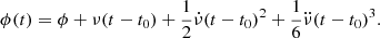
The additional phase in the pulsar rotation due to the glitch behaviour can be described in the timing model as (Mcculloch et al. 1987):
![$$ \begin{aligned} \phi _\mathrm{g} (t)&= \Delta \phi + \Delta \nu _\mathrm{p} (t-t_\mathrm{g} ) + \frac{1}{2} \Delta \dot{\nu }_\mathrm{p} (t-t_\mathrm{g} )^2 + \nonumber \\&\quad \frac{1}{6} \Delta \ddot{\nu }(t-t_\mathrm{g} )^3 + \sum _i \left[1-\exp {\left(-\frac{t-t_\mathrm{g} }{\tau ^{i}_\mathrm{d} }\right)} \right]\Delta \nu ^{i}_\mathrm{d} \, \tau _\mathrm{d} ^{i}. \end{aligned} $$](/articles/aa/full_html/2025/06/aa54098-25/aa54098-25-eq6.gif)
Here, Δϕ is the offset in the pulsar phase that helps counteract the uncertainty in the glitch epoch tg. The permanent jumps in ν and its derivatives with respect to the pre-glitch solution are Δνp,  and
and  . The transient increments in the frequency are described with Δνd, and decay after a timescale τd. For a Vela glitch, the highest number of transient components found so far is four3.
The instantaneous changes in ν and  at the glitch epoch can be described as

Then, the degree of recovery of the glitch, Q, is characterised by relating the transient and permanent jumps in frequency as Q = Δνd/Δνg.
4. 2024 Vela glitch characterisation
In Zubieta et al. (2024c) we first reported the detection of a new (#23) glitch in the Vela pulsar. The 22 glitches previously reported are listed in the ATNF catalogue4.
On April 28, we observed the Vela pulsar between MJD 60428.8386 and MJD 60428.9973. We observed 220 minutes using A1 and 216 minutes using A2 and measured a barycentric period of Pbary = 89.426459082(89) ms which was consistent with the ephemeris at that moment. We did not observe a glitch during that observation. Then, we observed the Vela pulsar again on MJD 60431.8304 and measured a period of Pbary = 89.426366478(76) ms, which shows a decrease with respect to the expected period of ΔP = 0.239 μs. We first placed the glitch epoch between MJD 60428.96 (2024-04-28 23h UTC) and MJD 60431.84 (2024-05-01 20h UTC). Later the glitch epoch was constrained to MJD 60429.86962(4) (Palfreyman 2024), which we have adopted in our timing solution.
In this work, we exhibit a deeper examination of the Vela timing behaviour near the glitch epoch. We focused on a small (∼70 d) time window close to the glitch to roughly characterise short-term behaviour of the glitch and avoid the effects of the strong red noise experienced by the Vela pulsar. We included 40 observations made with A1 and 23 observations made with A2. We obtained 4 ToAs (∼1 TOA per hour) from each observation and characterised the white noise using TEMPONEST (Lentati et al. 2014) to obtain the parameters TNGlobalEF and TNGlobalEQ (Li et al. 2016). The first one captures the impact of unaccounted for instrumental effects and imperfect estimations of TOA uncertainties, while the latter one addresses any additional sources of time independent uncertainties, such as pulse jitter. We obtained TNGlobalEF = 4.1283 which is the factor by which the template-fitting underestimates the ToA errorbars and TNGlobalEQ = −5.64459 which indicates a systematic uncertainty of 2 μs.
In order to obtain a full-timing solution for the glitch, we followed a procedure similar to what we did in Zubieta et al. (2023). We first obtained the pre-glitch rotational model by fitting ν,  and
and  to the TOAs before the glitch, keeping the value of the dispersion measure DM = 67.93(1) pc cm−3 as extracted from the ATNF pulsar catalogue. We show the residuals corresponding to the pre-glitch timing model in Fig. 1a. We then fit to the TOAs the permanent jumps in ν and
  (Δν and
  ) in Eq. (2).
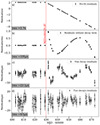 |
Fig. 1. Vela’s timing model with the parameters from Table 1. Panel a: Residuals without including the glitch in the timing model. Panel b: Residuals after fitting for Δν and |

The timing residuals shown in Fig. 1b revealed the presence of a recovery term. We used the GLITCH plug-in in TEMPO2 to estimate τd1 ∼ 17 d. We included τd1 in the timing model together with νd1 and fitted the whole glitch model to the residuals. We still found a remaining structure in the residuals as shown in Fig. 1c. We ran the GLITCH plug-in again over these residuals and we found one extra recovery term of ∼2.8 d (see Table 1).
Parameters of the timing model for the 2024 April 29 Vela glitch and their (1σ) uncertainties.
Considering the difficulty of TEMPO2 to fit recovery terms to the TOAs, we looked for the best combination of τd1 and τd2 as in the method described in Zubieta et al. (2023). Considering the values of the recoveries found through the GLITCH plug-in, we defined ranges for τd1 and τd2 between 0.5 and 30 days for both of them, and fitted Δϕ, Δν,  , Δνd1 and Δνd2 for every possible combination of τd1 and τd2 in those ranges. We searched for the glitch timing model that minimised the reduced chi-squared of the timing residuals (χred2 = χ2/d.o.f.), where d.o.f. are the degrees of freedom. We then systematically shortened the ranges for τd1 and τd2 and arrived to the solution that we show in Fig. 2, where we calculated the 1σ, 2σ and 3σ errorbars following Press et al. (1992). We obtained τd1 = 17.3(3) d and τd2 = 2.78(3) d, with a degree of recovery of Q1 = 0.562(2)% and Q2 = 0.462(1)% respectively. In this case, the degree of recovery for the first and second recovery scale are similar, and the sum of both recoveries is around 1% of the total glitch size.
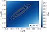 |
Fig. 2. Best fit of the decay time constants τd1 and τd2 for the 2024 Vela glitch. The solid line, dashed line, and dot-dashed line indicate the 1σ, 2σ, and 3σ confidence regions respectively. |
We plotted the residuals with the best solution in Fig. 1d. Residuals are flat indicating that the glitch timing model is consistent with our data. We did not find evidence of a step change in  during the glitch. The full timing model is shown in Table 1.
In Zubieta et al. (2024d) we reported a third large recovery term for the 2021 Vela glitch. Together with the two decays terms that we report in this work for the 2024 Vela glitch, we update in Fig. 3 all the recovery terms reported so far for Vela glitches. It is interesting to note that the third recovery time scale that we reported in Zubieta et al. (2024d) for the 2021 glitch, is not only the largest time scale reported so far but also it has the highest degree of recovery. This remarks the importance of re-analysing glitches with the whole post-glitch data span (until the following glitch arrives).
In addition, Fig. 3 shows that, except for two data points, the degree of recovery appears to increase with the recovery timescale. It is important to consider that there is an observational bias (and degeneracy) regarding both the number of decaying components being fitted and the corresponding timescales obtained (Antonopoulou et al. 2022). Therefore, it is important to keep revising glitch solutions to better constrain this effect and gain insight into the behaviour of the neutron star interior. For example, the need to fit multiple exponential components with different timescales, in terms of the vortex creep model, suggests that different regions within the neutron star respond to the glitch according to their own intrinsic properties (Alpar et al. 1993; Gügercinoğlu & Alpar 2020). By improving our understanding of these timescales, we could better interpret how the spatial distribution of the pinning forces affects the overall relaxation process.
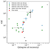 |
Fig. 3. Comparison of current and previous glitches decaying parameters for Vela pulsar. |
5. Analysis Methods: Pulse-by-pulse analysis of the 2021 Vela glitch
In this section, we report the analysis of the observations around the Vela glitch pulse by pulse. High-resolution single-pulse micro-structure pulse studies of the Vela pulsar were reported in Johnston et al. (2001) and Cairns et al. (2001), while the temporal evolution of the pulses for large timescales was studied in Palfreyman et al. (2016). Here we take advantage of the large amount of our daily data, which is well suited for statistical and machine learning studies. Our approach has been carried out using a combination of the VAE reconstruction and the SOM clustering techniques (Kingma & Welling 2014; Kohonen 1988).
We analysed nine observations in 2024, five before the glitch, on April 17, 18, 19, 20, and 28, and four after the glitch, on May 1, 2, 3, and 4. All observations were carried out with A2 in dual polarisation in the 1400–1456 MHz band. The number of pulses in each observation is given in Table 2. Those are uninterrupted single observations with A2 antenna observations typically lasting 3.66 hours. All observations were folded with a fixed DM = 67.93(1) pc cm−3 from the ATNF catalogue5 (as we have seen very small variations during each observation, DM < 0.2 pc cm−3) and cleaned from radio frequency interferences using RFIClean (Maan et al. 2021) with protection of the fundamental frequency of Vela (11.184 Hz). The complete procedure is described in Appendix C of Lousto et al. (2021), where we found that using rfifind (a task within PRESTO; Ransom 2018) on the data output from RFIClean further improves the SNR in most of the cases we studied. The amplitudes of the pulses are in arbitrary units as we did not observe any flux calibrator. Their relative distribution, day per day analysed here (Table 2), is displayed in Fig. 4. We note the qualitative similarities of the A2 pulse distributions pre-glitch on top, while the post-glitch observations are a bit more heterogeneous. For a more quantitative comparison, one can look at the parameters of the clusters in the tables in Appendix A.
Days of observation around the 2024 April 29 Vela glitch.
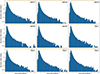 |
Fig. 4. Peak amplitude of single pulses distribution for observations with A2 preglitch on April 17–20,28, and post glitch on May1–5, 2024. The top yellow curve is the cumulative sum. |
5.1. Self-Organizing Map (SOM) techniques
In Lousto et al. (2021), Zubieta et al. (2023) we described a deep learning generative and clustering method built on Variational AutoEncoders (VAE) and Self-Organizing Maps (SOM) to perform Vela per-pulse clustering in an unsupervised manner.
For our method, we employ a two-stage process where the raw noisy pulses are first de-noised (VAE) and then are grouped into clusters second (SOM). The raw noisy pulses X are denoised into smooth approximations X̂ through neural networks that compress the input into a lower-dimensional stochastic space and then try to reconstruct the signal. We then define a 2D grid of M nodes, V1 : M, each initialised as a random vector in data space. The grid is iteratively updated through a competitive process where the input signals are presented to all nodes and the closest node, determined by Euclidean distance, is chosen as the ‘best matching unit’. This node and its grid neighbours are then slightly pulled closer to that input data point. This process is repeated until the grid is stable. The result is a set of cluster centres and assignments that partition similar signals into groups based on the dataset’s latent structure. The schematic diagrams of VAE and the usage of SOM for clustering are presented in Fig. 11 of Lousto et al. (2021).
5.2. Results
In Figure 5 we display the detail of the pulse clustering for the available days of observation just before (April 28) and just after (May 1) the glitch on April 29. We also have collected the results of the SOM clustering for the total nine days of observation in the Appendix A in Figs. A.1 and A.2. The results are displayed by days in successive rows and the three columns correspond to the choice of collecting the whole set of pulses in 4, 6, and 9 clusters respectively. The glitch, which occurred on 2024 April 29, happened after the observations displayed in Fig. A.1 and before those observations displayed in Fig. A.2. We have chosen the same vertical scale to represent the mean pulse of each cluster over the choices of the number of clusters and over the days of observation in order to exhibit the relative amplitudes, also affected by the different amounts of observing time. Figures A.1 and A.2, display pulses amplitudes (in the arbitrary units coming from the PRESTO (FFT) normalisation). We have not used standard sources to seek a normalisation of the observations, although we report the signal-to-noise ratio (SNR) of each observation as provided by PRESTO in Table 2.
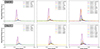 |
Fig. 5. Mean cluster reconstruction for observations with A2 just before and after the glitch on 2024, April 28, and May 1, using 4, 6, and 9 SOM clustering. |
The labelling of the clusters in each panel is ordered from the largest to the lowest amplitude mean pulse, while cluster 0 is the total mean pulse of the whole observation and remains the same over the three horizontal panels as a reference value. We first note an increase in the amplitude of the mean pulse of the cluster 1 as we increase the number of clusters allowed to SOM. They also decrease the number of pulses per cluster (as expected), which explains the amplitude increase. This behaviour is shared by clusters 2 and 3, and successively. We also note an earlier arrival and a mild decrease in the width of the high amplitude clusters (feature that could be used for improved timing in other circumstances or for other millisecond pulsars as we noted in Lousto et al. 2021). These points are more precisely quantified, with estimated errors, in the tables presented in Appendix A.
On the other hand, as seen in the tables in Appendix A, we have not found any notable qualitative systematic changes in the clustering during the days just before and after the glitch. We hence conclude that the effects of the glitch on the pulses might be either subtler and, or, of shorter time scale around the glitch time and we will continue to monitor Vela to capture the next event live as in the case of the 2016 glitch (Ashton et al. 2019).
6. Conclusions and discussion
Here we presented a detailed analysis of the latest (#23 recorded) large Vela glitch, first reported in Zubieta et al. (2024c), finding for this 2024 glitch a (Δνg/ν)2024 = 2.4 × 10⁻⁶, comparable with the values for the previous 2019 and 2021 glitches. We are able to provide an accurate description of the glitch characteristic epoch, jumps, and exponential recoveries with timescales of 17.3 and 2.78 d, respectively (see Table 1 and Fig. 3). In 2019 we reported a large Vela (#21 recorded) glitch (Lopez Armengol et al. 2019; Gancio et al. 2020) with a (Δνg/ν)2019 = 2.7 × 10⁻⁶. More recently, in Sosa-Fiscella et al. (2021), Zubieta et al. (2023) we presented a detailed analysis of the (#22 recorded) 2021 Vela glitch, with (Δνg/ν)2021 = 1.2 × 10⁻⁶ and exponential recoveries with associated timescales of 6.4 and 1 d, respectively.
The high cadence of our observations allowed us to verify and independently estimate the time of the glitch as, tg(MJD) = 60429.86961(4), confirming the value initially reported in Palfreyman (2024). Furthermore, the accuracy of our observations also allowed us to perform pulse-by-pulse studies of Vela using the machine learning techniques previously validated in Lousto et al. (2021), Zubieta et al. (2023).
For the sake of direct comparison among Vela’s last two large glitches we have paralleled the pulse-by-pulse analysis of this 2024 Vela glitch with that of the 2021 in Lousto et al. (2021), Zubieta et al. (2023). We note in Figs. A.1–A.2 that the higher amplitude pulse clusters tend to appear earlier and are narrower than the bulk of the other pulses (see also tables in Appendix A). This is particularly rigorous cluster by cluster in the four cluster analysis and typically large amplitude clusters are narrower by a factor ∼2 and the errors are nearly an order of magnitude smaller than for the whole set of pulses. We note that these four-cluster distributions follow a similar pattern in the sense to our previous studies with observations about six months before the 2021 glitch, on 2021 January 21, 24, 28 and March 29 (Lousto et al. 2021) and around the 2021 glitch on July 22 2021 and on July, 19, 20, 21, 23, and 24 (Zubieta et al. 2023); and it was associated with strata of the magnetosphere at different highs separated by ∼100 km (Lousto et al. 2021). Figure 6 displays the results of applying this model to each of the four days of observation for each antenna. The right-hand-side ordinate gives the components distances to the average pulse reference height in the pulsar magnetosphere. We note the consistency between the components for each of the four days and for each individual antenna’s observations. The four components appear to be almost equidistant (this maybe an effect of the SOM clustering method) and roughly of the order of ∼100 kilometres. We also note that new independent recent studies confirm this early arrival of high amplitude pulses Mahida et al. (2023).
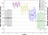 |
Fig. 6. Peak location and conversion to magnetosphere altitude, with the corresponding error bars, per day for each of the 4 clusters and for the whole observation. |
We finally note the much smaller error bars displayed in Fig. 6 in the pulse peak determination for the larger amplitude pulsar cluster (labelled as #1) than for the whole observation (labelled as #0), thus opening the possibility to use this cluster for timing of pulsars in order to achieve much higher precision of its timing measurements.
Acknowledgments
We especially thank Yogesh Maan for numerous beneficial discussions about the best use of RFIClean. COL gratefully acknowledge the National Science Foundation (NSF) for financial support from Grants No. PHY-2207920, and AST-2319326. JAC and FG are CONICET researchers. JAC and FG acknowledge support from PIP 0113 (CONICET). JAC and FG were also supported by grant PID2019-105510GB-C32/AEI/10.13039/501100011033 from the Agencia Estatal de Investigación of the Spanish Ministerio de Ciencia, Innovación y Universidades, and by Consejería de Economía, Innovación, Ciencia y Empleo of Junta de Andalucía as research group FQM-322, as well as FEDER funds. FG acknowledges support from PIBAA 1275 (CONICET).
References
- Alpar, M. A., Chau, H. F., Cheng, K. S., & Pines, D. 1993, ApJ, 409, 345 [Google Scholar]
- Andersson, N., Glampedakis, K., Ho, W. C. G., & Espinoza, C. M. 2012, Phys. Rev. Lett., 109, 241103 [NASA ADS] [CrossRef] [Google Scholar]
- Antonopoulou, D., Haskell, B., & Espinoza, C. M. 2022, Rep. Prog. Phys., 85, 126901 [NASA ADS] [CrossRef] [Google Scholar]
- Araujo Furlan, S. B., Gancio, G., Galante, C. A., & Romero, G. E. 2023, Boletin de la Asociacion Argentina de Astronomia La Plata Argentina, 64, 304 [Google Scholar]
- Ashton, G., Lasky, P. D., Graber, V., & Palfreyman, J. 2019, Nat. Astron., 3, 1143 [Google Scholar]
- Basu, A., Shaw, B., Antonopoulou, D., et al. 2022, MNRAS, 510, 4049 [NASA ADS] [CrossRef] [Google Scholar]
- Bransgrove, A., Beloborodov, A. M., & Levin, Y. 2020, ApJ, 897, 173 [Google Scholar]
- Cairns, I. H., Johnston, S., & Das, P. 2001, ApJ, 563, L65 [Google Scholar]
- Chamel, N. 2013, Phys. Rev. Lett., 110, 011101 [NASA ADS] [CrossRef] [Google Scholar]
- Dodson, R. G., McCulloch, P. M., & Lewis, D. R. 2002, ApJ, 564, L85 [Google Scholar]
- Espinoza, C. M., Lyne, A. G., Stappers, B. W., & Kramer, M. 2011, MNRAS, 414, 1679 [NASA ADS] [CrossRef] [Google Scholar]
- Flanagan, C. S. 1990, Nature, 345, 416 [Google Scholar]
- Gancio, G., Lousto, C. O., Combi, L., et al. 2020, A&A, 633, A84 [NASA ADS] [CrossRef] [EDP Sciences] [Google Scholar]
- Gancio, G., Romero, G. E., Astudillo, J., Saavedra, E. A., & Combi, J. A. 2024, Rev. Mex. Astron. Astrofis. Conf. Ser., 56, 131 [Google Scholar]
- Graber, V., Cumming, A., & Andersson, N. 2018, ApJ, 865, 23 [Google Scholar]
- Gügercinoğlu, E. 2017, J. Phys. Conf. Ser., 932, 012037 [Google Scholar]
- Gügercinoğlu, E., & Alpar, M. A. 2020, MNRAS, 496, 2506 [CrossRef] [Google Scholar]
- Haskell, B., & Melatos, A. 2015, Int. J. Mod. Phys. D, 24, 1530008 [NASA ADS] [CrossRef] [Google Scholar]
- Ho, W. C. G., Espinoza, C. M., Antonopoulou, D., & Andersson, N. 2015, Sci. Adv., 1, e1500578 [Google Scholar]
- Hobbs, G., Coles, W., Manchester, R. N., et al. 2012, MNRAS, 427, 2780 [NASA ADS] [CrossRef] [Google Scholar]
- Hotan, A. W., van Straten, W., & Manchester, R. N. 2004, PASA, 21, 302 [Google Scholar]
- Johnston, S., van Straten, W., Kramer, M., & Bailes, M. 2001, ApJ, 549, L101 [NASA ADS] [CrossRef] [Google Scholar]
- Khomenko, V., & Haskell, B. 2018, PASA, 35, e020 [Google Scholar]
- Kingma, D. P., & Welling, M. 2014, arXiv e-prints [arXiv:1312.6114] [Google Scholar]
- Kohonen, T. 1988, Self-Organized Formation of Topologically Correct Feature Maps (Cambridge, MA, USA: MIT Press), 509 [Google Scholar]
- Lentati, L., Alexander, P., Hobson, M. P., et al. 2014, MNRAS, 437, 3004 [NASA ADS] [CrossRef] [Google Scholar]
- Li, L., Wang, N., Yuan, J. P., et al. 2016, MNRAS, 460, 4011 [NASA ADS] [CrossRef] [Google Scholar]
- Link, B., Epstein, R. I., & Lattimer, J. M. 1999, Phys. Rev. Lett., 83, 3362 [Google Scholar]
- Lopez Armengol, F. G., Lousto, C. O., del Palacio, S., et al. 2019, ATel, 12482, 1 [NASA ADS] [Google Scholar]
- Lorimer, D. R., & Kramer, M. 2004, Handbook of Pulsar Astronomy, 4 (Cambridge) [Google Scholar]
- Lousto, C. O., Missel, R., Prajapati, H., et al. 2021, MNRAS, stab3287 [Google Scholar]
- Lyne, A. G. 1992, Phil. Trans. R. Soc. London Ser. A, 341, 29 [Google Scholar]
- Maan, Y., van Leeuwen, J., & Vohl, D. 2021, A&A, 650, A80 [NASA ADS] [CrossRef] [EDP Sciences] [Google Scholar]
- Mahida, A. D., Palfreyman, J. L., Calves, G. M., & Sett, S. 2023, MNRAS, 524, 759 [Google Scholar]
- Manchester, R. N. 2018, in Pulsar Astrophysics the Next Fifty Years, eds. P. Weltevrede, B. B. P. Perera, L. L. Preston, & S. Sanidas, IAU Symp., 337, 197 [NASA ADS] [Google Scholar]
- Manchester, R. N., Hobbs, G. B., Teoh, A., & Hobbs, M. 2005, AJ, 129, 1993 [Google Scholar]
- Mcculloch, P., Klekociuk, A., Hamilton, P., & Royle, G. 1987, Aust. J. Phys., 40, 725 [Google Scholar]
- Montoli, A., Antonelli, M., & Pizzochero, P. M. 2020, MNRAS, 492, 4837 [Google Scholar]
- Palfreyman, J. 2024, ATel, 16615, 1 [Google Scholar]
- Palfreyman, J. L., Dickey, J. M., Ellingsen, S. P., Jones, I. R., & Hotan, A. W. 2016, ApJ, 820, 64 [Google Scholar]
- Palfreyman, J., Dickey, J. M., Hotan, A., Ellingsen, S., & van Straten, W. 2018, Nature, 556, 219 [NASA ADS] [CrossRef] [Google Scholar]
- Press, W. H., Teukolsky, S. A., Vetterling, W. T., & Flannery, B. P. 1992, Numerical Recipes in C. The Art of Scientific Computing (IOP Publishing) [Google Scholar]
- Radhakrishnan, V., & Manchester, R. N. 1969, Nature, 222, 228 [NASA ADS] [CrossRef] [Google Scholar]
- Ransom, S. 2011, Astrophysics Source Code Library [record ascl:1107.017] [Google Scholar]
- Ransom, S. 2018, PRESTO - Pulsar Exploration and Search Toolkit [Google Scholar]
- Reichley, P. E., & Downs, G. S. 1969, Nature, 222, 229 [NASA ADS] [CrossRef] [Google Scholar]
- Schubert, E., Sander, J., Ester, M., Kriegel, H., & Xu, X. 2017, ACM Trans. Database Syst., 42, 1 [CrossRef] [Google Scholar]
- Sosa-Fiscella, V., Zubieta, E., del Palacio, S., et al. 2021, ATel, 14806, 1 [Google Scholar]
- Taylor, J. H. 1992, Phil. Trans. R. Soc. London, 341, 117 [Google Scholar]
- Yu, M., Manchester, R. N., Hobbs, G., et al. 2013, MNRAS, 429, 688 [NASA ADS] [CrossRef] [Google Scholar]
- Zubieta, E., Del Palacio, S., Garcia, F., et al. 2022a, ATel, 15638, 1 [NASA ADS] [Google Scholar]
- Zubieta, E., Furlan, S. B. A., Palacio, S. d., et al. 2022b, ATel, 15838, 1 [Google Scholar]
- Zubieta, E., Missel, R., Sosa Fiscella, V., et al. 2023, MNRAS, 521, 4504 [Google Scholar]
- Zubieta, E., Araujo Furlan, S. B., del Palacio, S., et al. 2024a, ATel, 16580, 1 [Google Scholar]
- Zubieta, E., del Palacio, S., García, F., et al. 2024b, Rev. Mex. Astron. Astrofis. Conf. Ser., 56, 161 [NASA ADS] [Google Scholar]
- Zubieta, E., Furlan, S. B. A., Palacio, S. d., et al. 2024c, ATel, 16608, 1 [Google Scholar]
- Zubieta, E., García, F., del Palacio, S., et al. 2024d, A&A, 689, A191 [NASA ADS] [CrossRef] [EDP Sciences] [Google Scholar]
- Zubieta, E., García, F., del Palacio, S., et al. 2025, A&A, 694, A124 [NASA ADS] [CrossRef] [EDP Sciences] [Google Scholar]
Appendix A: Tables of SOM Clustering
In Tables A.1.–A.9. we describe in detail the six-cluster analysis of the observations on the days april-17-2024-A2, april-18-2024-A2, april-19-2024-A2, april-20-2024-A2, april-28-2024-A2, before the glitch and may-01-2024-A2, may-02-2024-A2, may-03-2024-A2, and may-04-2024-A2, after the glitch.
SOM Clustering for April 17 with Antenna A2.
SOM Clustering for April 18 with Antenna A2.
SOM Clustering for April 19 with Antenna A2.
SOM Clustering for April 20 with Antenna A2.
SOM Clustering for April 28 with Antenna A2.
SOM Clustering for May 01 with Antenna A2.
SOM Clustering for May 02 with Antenna A2.
SOM Clustering for May 03 with Antenna A2.
SOM Clustering for May 04 with Antenna A2.
Here we include the numerical information in tabular form about the clustering analysis summarised in Fig. A.1-A.2 below. They include a 6 SOM clusters decomposition as representative for each of the days of observation. We provide the number of pulses of each cluster # pulses; peak location from the index of the maximum value in the pulse sequence; peak height from the maximum value of the pulse sequence; peak width done by first finding the maximum value of the sequence, then performing full-width half maximum of peak; (library used for this: https://docs.scipy.org/doc/scipy/reference/generated/scipy.signal.peak_widths.html); for the peak skew we evaluated the Fisher-Pearson coefficient of skewness; (using the scipy for this computation https://docs.scipy.org/doc/scipy/reference/generated/scipy.stats.skew.html); The cluster #0 corresponds to the total number of pulses in the observation and the successive clusters from #1 to the #6 SOM clustering are ordered accordingly to the highest peak amplitude of the mean pulse computed for each cluster and represented in Figs. A.1-A.2. We compute the peak location with respect to our grid of bins (here centred at around 100 for cluster #0) and totalling 611 bins per period, giving us a time resolution of 146 μs. We also provide a measure of the pulse width as given by the standard deviation (σ) and its skewness, all with estimated 1σ errors, and finally MSE is the standard mean squared error  , the average per-step mean squared reconstruction error over all sequences. We observe a systematic tendency for the pulses’ peaks to appear earlier the higher the amplitude as well as a reduction of its width and an increase of the skew (also observed in the previous work of Lousto et al. (2021), Zubieta et al. (2023) analysing 2021 observations.
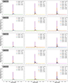 |
Fig. A.1. Mean cluster reconstruction for observations with A2 before the glitch on 2024, April 17, 18, 19, 20, and 28, using 4, 6, and 9 SOM clustering. [200 (out of total 611) phase bins were taken around the mean peak (at bin 100) of each day to perform the single-pulse analysis]. |
Here we include all the days of observation used in the 4, 6, and 9 SOM clustering analysis summarised in Fig. A.1-A.2.
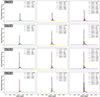 |
Fig. A.2. Mean cluster reconstruction for observations with A2 after the glitch on 2024, May 1, 2, 3, and 4, using 4, 6, and 9 SOM clustering. [200 (out of total 611) phase bins were taken around the mean peak (at bin 100) of each day to perform the single-pulse analysis]. |
Appendix B: VAE reconstruction and SOM Clustering for April 28 observation with A2
In order to show that what we observe with the clusters baseline is not an artefact of the VAE pulse reconstruction method, in Fig. B.1 we display some selected individual raw pulses belonging to the 4 SOM clusters versus their corresponding reconstructions showing the actual baseline fluctuations over the full period range. We also display the VAE representation of the four SOM clusters in Fig. B.2.
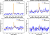 |
Fig. B.1. Individual pulse reconstructions from the April 28, 2024 observations with A2. One signal index is sampled from each of the four SOM clusters, with the VAE reconstruction shown alongside the corresponding raw observation. Individual pulse indices are # 47419, 36415, 35083, 53075, respectively. |
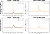 |
Fig. B.2. Mean reconstructions of individual signals for each of the four SOM clusters from the April 28, 2024 observations with A2. All signals are reconstructed individually using the VAE, then averaged and compared to the mean of the corresponding raw observations. |
All Tables
Parameters of the timing model for the 2024 April 29 Vela glitch and their (1σ) uncertainties.
All Figures
|
Fig. 1. Vela’s timing model with the parameters from Table 1. Panel a: Residuals without including the glitch in the timing model. Panel b: Residuals after fitting for Δν and |
| In the text | |
|
Fig. 2. Best fit of the decay time constants τd1 and τd2 for the 2024 Vela glitch. The solid line, dashed line, and dot-dashed line indicate the 1σ, 2σ, and 3σ confidence regions respectively. |
| In the text | |
|
Fig. 3. Comparison of current and previous glitches decaying parameters for Vela pulsar. |
| In the text | |
|
Fig. 4. Peak amplitude of single pulses distribution for observations with A2 preglitch on April 17–20,28, and post glitch on May1–5, 2024. The top yellow curve is the cumulative sum. |
| In the text | |
|
Fig. 5. Mean cluster reconstruction for observations with A2 just before and after the glitch on 2024, April 28, and May 1, using 4, 6, and 9 SOM clustering. |
| In the text | |
|
Fig. 6. Peak location and conversion to magnetosphere altitude, with the corresponding error bars, per day for each of the 4 clusters and for the whole observation. |
| In the text | |
|
Fig. A.1. Mean cluster reconstruction for observations with A2 before the glitch on 2024, April 17, 18, 19, 20, and 28, using 4, 6, and 9 SOM clustering. [200 (out of total 611) phase bins were taken around the mean peak (at bin 100) of each day to perform the single-pulse analysis]. |
| In the text | |
|
Fig. A.2. Mean cluster reconstruction for observations with A2 after the glitch on 2024, May 1, 2, 3, and 4, using 4, 6, and 9 SOM clustering. [200 (out of total 611) phase bins were taken around the mean peak (at bin 100) of each day to perform the single-pulse analysis]. |
| In the text | |
|
Fig. B.1. Individual pulse reconstructions from the April 28, 2024 observations with A2. One signal index is sampled from each of the four SOM clusters, with the VAE reconstruction shown alongside the corresponding raw observation. Individual pulse indices are # 47419, 36415, 35083, 53075, respectively. |
| In the text | |
|
Fig. B.2. Mean reconstructions of individual signals for each of the four SOM clusters from the April 28, 2024 observations with A2. All signals are reconstructed individually using the VAE, then averaged and compared to the mean of the corresponding raw observations. |
| In the text | |
Current usage metrics show cumulative count of Article Views (full-text article views including HTML views, PDF and ePub downloads, according to the available data) and Abstracts Views on Vision4Press platform.
Data correspond to usage on the plateform after 2015. The current usage metrics is available 48-96 hours after online publication and is updated daily on week days.
Initial download of the metrics may take a while.