© The Authors 2025

1. Introduction

The association of GW170817 and GRB 170817A confirmed that binary neutron star (BNS) mergers are the progenitors of some short gamma-ray bursts (Abbott et al. 2017). However, the nature of GW170817’s remnant remains uncertain, and various physical parameters can impact the lifetime of the merger remnant before its collapse into a black hole. Depending on the hot and dense matter equation of state and the masses of the neutron stars, different fates await the remnant after the merger: if the remnant mass M remains lower than the maximum mass of a nonrotating neutron star M_TOV, it stays indefinitely stable. Otherwise, the remnant can promptly collapse into a black hole, or it can form a hypermassive neutron star (HMNS) (Baumgarte et al. 2000), which is a neutron star that is stabilized by differential rotation while having a mass higher than the maximum mass of a uniformly rotating cold neutron star. An HMNS can either (i) collapse into a black hole when differential rotation is transported (Duez et al. 2006; Shibata et al. 2006), or (ii) be stabilized by solid body rotation, increasing M_TOV by around ∼20% (Cook et al. 1994a; Lasota et al. 1996; Breu & Rezzolla 2016; Musolino et al. 2024). In the latter case, the remnant is called a supramassive neutron star (Cook et al. 1994b) that collapses after spinning down by magnetic dipole radiation on a timescale ranging from minutes to hours, or even longer. In the following, we call the long-lived remnant case when the remnant survives for O(1) s and it often corresponds to the supramassive neutron star case.

After the merger of two neutron stars, the nature of the remaining object can significantly affect the electromagnetic counterparts due to various factors. In the case of an HMNS, these include powerful neutrino luminosity, strong magnetic fields (≥10¹⁵ G), and rotational kinetic energy reservoirs of order 10⁵³ erg. Several studies have examined the impact of these factors on post-merger events (e.g., Metzger et al. 2008; Bucciantini et al. 2012; Gao et al. 2013; Metzger & Piro 2014; Gompertz et al. 2014; Sarin et al. 2022). Magnetic fields, along with fast rotation, play a critical role in neutron star mergers as they can extract rotational kinetic energy and drive powerful relativistic outflows (e.g., Shibata et al. 2021; Combi & Siegel 2023; Kiuchi et al. 2024). Therefore, understanding the evolution of the magnetic field and the rotation profile of the HMNS is crucial for interpreting future multi-messenger observations.

During the first few milliseconds after the merger, the magnetic field of the HMNS is amplified by the Kelvin-Helmholtz instability due to the presence of the shear layer at the contact interface between the two neutron stars (Rasio & Shapiro 1999; Price & Rosswog 2006; Kiuchi et al. 2014, 2015; Aguilera-Miret et al. 2024). This generates a strong, small-scale magnetic field. However, another mechanism is necessary to get a large-scale magnetic field capable of driving an outflow. Both the magnetorotational instability (MRI) and the Tayler-Spruit (TS) dynamo could possibly fulfill this role, but act in different regions of the HMNS. Indeed, the remnant from the BNS merger has a rotation profile with an angular velocity that increases with radius until 10 km and then decreases afterwards (Shibata & Taniguchi 2006). Therefore, this rotation profile is unstable to the MRI at radii larger than 10 km. This instability is studied in the case of long-lived remnants, for which it is shown that it could drive a luminous relativistic outflow (Combi & Siegel 2023; Kiuchi et al. 2024). By contrast, the differential rotation is such that the flow is stable to the MRI at radii smaller than 10 km, and core regions could instead be unstable to a Tayler-instability driven dynamo (Tayler 1973; Spruit 2002).

The Tayler instability is a type of magnetic instability in flows of electrically conducting, stably stratified fluids where a strong azimuthal magnetic field can become unstable, causing disruptions due to the Lorentz forces that arise from the interaction of currents along the axis of symmetry and magnetic fields (Tayler 1973; Pitts & Tayler 1985). The first model of a dynamo driven by the Tayler instability was proposed by Spruit (2002) for stably stratified, differentially rotating regions. Fuller et al. (2019) have proposed an alternative description to address criticisms of Spruit’s model (see Denissenkov & Pinsonneault 2007; Zahn et al. 2007). For a long time, numerical simulations were unable to capture the TS dynamo, but recent numerical simulations have finally provided numerical evidence that this dynamo exists, both in the presence of negative shear (Petitdemange et al. 2023, 2024; Daniel et al. 2023) and positive shear (Barrère et al. 2023, 2025). The former set-up is more relevant to model stellar radiative interiors, where the Tayler instability is proposed to explain the angular momentum evolution of stellar interiors (Fuller et al. 2019) and the magnetic dichotomy observed in intermediate-mass and massive stars (Rüdiger & Kitchatinov 2010; Szklarski & Arlt 2013; Bonanno et al. 2020; Jouve et al. 2020). On the other hand, a positive shear (with a faster-rotating surface) can be encountered in proto-neutron stars (PNSs). In this context, the TS dynamo plays a central role in a new scenario explaining magnetar formation from slow-rotating progenitors (Barrère et al. 2022).

The TS is also proposed as a mechanism for angular momentum transport potentially leading to their collapse into black holes (Margalit et al. 2022). This study estimates the angular momentum transport timescale due to the transport by the saturated magnetic fields from analytical scalings but neglects the duration of the dynamo growth. However, neutrino viscosity could make the TS dynamo stable, or it could require more time to reach saturation than the lifetime of the HMNS.

Therefore, this paper aims to study whether the conditions in BNS merger remnants could allow the TS dynamo to grow and impact its evolution. In particular, this study applies a similar one-zone model to that of Barrère et al. (2022), within the framework of BNS mergers. The paper is organized as follows: in Sect. 2, we describe the modelling of the HMNS and the equations for a one-zone model of the TS dynamo. The results of the one-zone models are presented in Sect. 3, followed by a comparison to the recent super-high resolution GRMHD simulation from Kiuchi et al. (2024) in Sect. 4. Finally, we discuss the validity of our assumptions in Sect. 5 and conclude in Sect. 6.

2. A one-zone model of the Tayler-Spruit dynamo in the hypermassive neutron star

2.1. Modeling of the hypermassive neutron star

For our HMNS model, we use the data from a 3D GRMHD simulation with a stiff equation of state, DD2 (Hempel & Schaffner-Bielich 2010), where the remnant lasts for more than 0.15 s (Kiuchi et al. 2024) (see Sect. 4 for more detail). To assess whether the TS dynamo is relevant for this HMNS model, we look at the rotation profile of the HMNS at different times (see top panel of Fig. 1). The remnant displays a cylindrical rotation profile with a large region in positive differential rotation between a cylindrical radius of R = 5 km and R = 10 km¹, where the TS dynamo could grow. We stress that this rotation profile is typical of HMNSs in many different simulations (Shibata & Taniguchi 2006; Kastaun et al. 2016, 2017). To characterize the differential rotation, we use the shear rate

$$\begin{array}{c}\hfill q\equiv \frac{\mathrm{d}ln\mathrm{\Omega }}{\mathrm{d}lnR},\end{array}$$

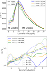Fig. 1. Top: Azimuthal averaged rotation profile of the remnant HMNS from the 3D GRMHD simulation as a function of the cylindrical radius, at different times t and vertical position z. Bottom: Averaged Brunt-Väisälä frequency of the remnant in the TS-unstable region as a function of the cylindrical radius, at different times t and different θ angles.

which means that a Keplerian shear corresponds to q = −1.5. In the following, we use the cylindrical radius R = 7 km as a typical radius for our thermodynamical quantities. At this radius, we have Ω = 5468 s⁻¹ and a shear rate of q = 1.12.

Since the TS dynamo requires a stable stratification, we test whether the core of the BNS remnant is convectively stable (Radice & Bernuzzi 2023). For that, we use the relativistic Ledoux criterion, given by

$$\begin{array}{c}\hfill C_{\mathrm{L}}=\frac{\partial \rho (1+ϵ)}{\partial r}-\frac{1}{c_{\mathrm{s}}^2}\frac{\partial P}{\partial r},\end{array}$$(1)

where ρ, ϵ, c_s and P are the density, specific internal energy, sound speed and pressure, respectively. We find that the HMNS is indeed stably stratified, and we use the general relativistic formula for the Brunt-Väisälä (BV) frequency N derived in Müller et al. (2013):

$$\begin{array}{c}\hfill N^2\equiv -c^2\frac{\alpha C_{\mathrm{L}}}{\rho h{\varphi }^4}\frac{\partial \alpha }{\partial r},\end{array}$$(2)

where α, h and ϕ are the lapse function, specific enthalpy, and conformal factor for the spatial metric: N is presented in the bottom panel of Fig. 1. Since it is rapidly rotating, the HMNS tends to be cylindrical. This means that the HMNS is more compact at the poles than at the equator, which leads to spherical radial gradients being stronger at the poles and a small increase in the Brunt-Väisälä frequency. This effect is more pronounced at larger radii as the frequency at r = 7 km stays relatively constant in theta. This formula comes from the hydrostatic equilibrium written as 𝒢 = −c²∇lnα, where, in the Newtonian limit, 𝒢 is the gravitational acceleration. Due to the rapid rotation, we prefer to use this definition of hydrostatic equilibrium rather than the one based on the pressure gradient for our background. With this formula, we find typical values of N = 4970 s⁻¹ at a radius of R_TI = 7 km for the Brunt-Väisälä frequency. The density is equal to ρ = 3.7 × 10¹⁴ g cm⁻³. Note that both the shear rate and the Brunt-Väisälä frequency defined here are not coordinate invariant.

In this context, we cannot assume that the rotational angular velocity Ω is much lower than the Brunt-Väisälä frequency. We also assume that the Alfvén frequency remains small compared to the rotation and Brunt-Väisälä frequencies,

$$\begin{array}{c}\hfill {\omega }_{\mathrm{A}}\equiv \frac{B}{\sqrt{4\pi \rho r^2}}\ll \mathrm{\Omega }\mathrm{and}{\omega }_{\mathrm{A}}\ll N\Rightarrow B\ll 2\times {10}^{17}\mathrm{G},\end{array}$$(3)

for the one-zone model. Note that this hypothesis may no longer be valid when we analyze the core dynamics in the GRMHD simulation, as the toroidal magnetic field can be winded to higher values. When these assumptions hold, the growth rate of the Tayler instability is σ_TI = ω_A²/Ω. In the case of slow rotation Ω ≪ ω_A, the growth rate is σ_TI = ω_A.

2.2. Newtonian Tayler-Spruit picture

As in Barrère et al. (2022), we decompose the velocity and magnetic field components into axisymmetric components, denoted as B_i or v_i and non-axisymmetric components, denoted as δB_i and δv_i. We justify the Newtonian approach in the Appendix.

The shear rate evolution due to angular momentum transport by Maxwell stresses is written as

$$\begin{array}{c}\hfill {\partial }_{t}q=-{\gamma }_{\mathrm{AM}}q=\frac{T_{\mathrm{R}\varphi }^{\mathrm{MAX}}}{4\pi \rho \mathrm{\Omega }{R}_{\mathrm{TI}}^2}=-\frac{B_{\mathrm{R}}{B}_{\varphi }}{4\pi \rho \mathrm{\Omega }{R}_{\mathrm{TI}}^2},\end{array}$$(4)

where $T_{\mathit{ij}}^{\mathrm{MAX}}$ is the Maxwell stress tensor. For the evolution of the angular velocity, we consider that the initial value decreases due to the magnetic torque. We also express it in terms of the Maxwell stress tensor, which gives

$$\begin{array}{c}\hfill {\partial }_t\mathrm{\Omega }=\frac{R_{\mathrm{TI}}^3{T}_{\mathrm{R}\varphi }^{\mathrm{MAX}}}{I}=-\frac{R_{\mathrm{TI}}^3{B}_{\mathrm{R}}{B}_{\varphi }}{I},\end{array}$$(5)

where I = 1.667 × 10⁴⁵ g cm² is the moment of inertia of the inner zone below 10 km. This means that in the case of a strong magnetic field, the rotation rate could decrease fast and be in the regime Ω ≪ ω_A. In the following, we keep the growth rate of the Tayler instability σ_TI that is equal to

$$\begin{array}{c}\hfill {\sigma }_{\mathrm{TI}}=\{\begin{array}{cc}{\omega }_{\mathrm{A}}\hfill & \mathrm{if}\mathrm{\Omega }\le {\omega }_{\mathrm{A}},\hfill \\ {\omega }_{\mathrm{A}}^2/\mathrm{\Omega }\hfill & \mathrm{if}{\omega }_{\mathrm{A}}\ge \mathrm{\Omega },\hfill \end{array}\end{array}$$(6)

in the evolution equations (Eqs. (7), (12) and (14)) of the magnetic field. For the dissipation of the perturbed magnetic field, we consider the same damping rate ${\gamma }_{\mathrm{cas}}\sim \frac{\delta v_{\mathrm{A}}}{r}$ as Fuller et al. (2019), where $\delta v_{\mathrm{A}}\equiv \frac{\delta B_{\varphi }}{\sqrt{4\pi \rho }}$ is the Alfvén velocity of the non-axisymmetric δB_ϕ. It comes from the cascade rate of the perturbed magnetic field towards smaller scales. The evolution equation of δB_ϕ is therefore

$$\begin{array}{c}\hfill {\partial }_t\delta B_{\varphi }=({\mathcal{B}}_{\mathrm{TI}}{\sigma }_{\mathrm{TI}}-{\gamma }_{\mathrm{cas}})\delta B_{\varphi }={\mathcal{B}}_{\mathrm{TI}}{\sigma }_{\mathrm{TI}}\delta B_{\varphi }-\frac{\delta v_{\mathrm{A}}}{R_{\mathrm{TI}}}\delta B_{\varphi },\end{array}$$(7)

where ℬ_TI is a boolean that describes whether the HMNS is unstable to the Tayler instability (see Eq. (24)). In the case of ideal MHD, the instability is stabilized when the magnetic tension due to the radial magnetic field, ∼k_TIB_RδB, where k_TI is the wavenumber of the Tayler instability, overcomes the driving force of the Tayler instability, the magnetic tension due to the toroidal magnetic field ∼m/rB_ϕδB, with m = 1 being the main mode of the Tayler instability (Fuller et al. 2019; Skoutnev & Beloborodov 2024). We have therefore

$$\begin{array}{c}\hfill {\mathcal{B}}_{\mathrm{TI}}=\{\begin{array}{cc}0\hfill & \mathrm{if}{B}_{\mathrm{R}}/B_{\varphi }>{\omega }_{\mathrm{A}}/N,\hfill \\ 1\hfill & \mathrm{otherwise}.\hfill \end{array}\end{array}$$(8)

One other difference between the HMNS model and the PNS model of Barrère et al. (2022) is the geometry: the rotation profile in an HMNS is cylindrical while it is spherical for a late stage of the PNS with fallback accretion. In our study, we, therefore, consider the cylindrical radial field B_R instead of the spherical radial field. The derivation of the equations is almost the same as it is just adapted to cylindrical coordinates. With a cylindrical differential rotation, the growth of the toroidal field B_ϕ is due to the winding of the cylindrical radial field B_R, described by ∂_tB_ϕ|_winding = qΩB_R. The growth rate of the toroidal field is therefore σ_shear = qΩB_R/B_ϕ. As in Barrère et al. (2022), we estimate the dissipation rates of B_R and B_ϕ by the non-linear magnetic energy dissipation rate ${\dot{E}}_{\mathrm{mag}}$ following

$$\begin{array}{c}\hfill {\gamma }_{\mathrm{diss}}\equiv \frac{{\dot{E}}_{\mathrm{mag}}}{B_{\varphi }^2},\end{array}$$(9)

where the radial magnetic field is neglected compared to the dominant azimuthal field such that we can estimate ${\dot{E}}_{\mathrm{mag}}\sim B_{\varphi }{\partial }_t{B}_{\varphi }$. The change in axisymmetric magnetic energy is due to the growth of the Tayler instability, and thus, we have

$$\begin{array}{c}\hfill {\dot{E}}_{\mathrm{mag}}\sim {\sigma }_{\mathrm{TI}}{|\delta B_{\varphi }|}^2.\end{array}$$(10)

It finally gives a dissipation rate

$$\begin{array}{c}\hfill {\gamma }_{\mathrm{diss}}\sim {\sigma }_{\mathrm{TI}}{\left(\frac{\delta B_{\varphi }}{B_{\varphi }}\right)}^2.\end{array}$$(11)

We take the simplification in order of magnitude of δB_⊥ ∼ δB_ϕ, as δB_⊥ is not well defined for cylindrical coordinates. The evolution equation of B_ϕ is therefore

$$\begin{array}{c}\hfill {\partial }_t{B}_{\varphi }=({\sigma }_{\mathrm{shear}}-{\gamma }_{\mathrm{diss}})B_{\varphi }=q\mathrm{\Omega }{B}_{\mathrm{R}}-{\sigma }_{\mathrm{TI}}\frac{\delta B_{\varphi }^2}{B_{\varphi }}·\end{array}$$(12)

In cylindrical coordinates, the growth rate σ_NL of B_R comes from non-linear effects of the perturbed magnetic field and velocity. This corresponds to the toroidal component of the electromotive force ℰ_ϕ that is given by

$$\begin{array}{c}\hfill \frac{\partial B_{\mathrm{R}}}{\partial t}=-\frac{\partial {\mathcal{E}}_{\varphi }}{\partial z}\sim \frac{{\mathcal{E}}_{\varphi }}{L_z},\end{array}$$(13)

where L_z is the vertical wavelength of the Tayler instability. By definition, in cylindrical coordinates, the toroidal component of the electromotive force is given by ℰ_ϕ = δv_RδB_z − δv_zδB_R. As in Barrère et al. (2022), we assume ℰ_ϕ ∼ δv_RδB_z ∼ δv_RδB_⊥ ∼ δv_RδB_ϕ. By assuming a magnetostrophic balance between the Lorentz and Coriolis forces, which gives δv_⊥Ω ∼ δv_Aω_A, we retrieve the same formula as previous studies in spherical geometry if we assume L_z ∼ R_TI, which we do for simplicity. For consistency, we also assume that the non-linear growth rate of the axisymmetric radial field is zero when the HMNS is stable to the Tayler instability. The evolution equation of B_R is therefore

$$\begin{array}{c}\hfill {\partial }_t{B}_{\mathrm{R}}=({\sigma }_{\mathrm{NL}}-{\gamma }_{\mathrm{diss}})B_{\mathrm{R}}={\mathcal{B}}_{\mathrm{TI}}\frac{{\omega }_{\mathrm{A}}^2}{N\mathrm{\Omega }}\frac{\delta B_{\varphi }^2}{\sqrt{4\pi \rho R_{\mathrm{TI}}^2}}-{\sigma }_{\mathrm{TI}}{\left(\frac{\delta B_{\varphi }}{B_{\varphi }}\right)}^2{B}_{\mathrm{R}}.\end{array}$$(14)

Overall, the magnetic field evolution is governed by equations similar to the equations of Barrère et al. (2022), with some changes to take into account the growth rate and the stabilization of the instability.

2.3. Impact of diffusive processes on the Tayler-Spruit dynamo

In an HMNS, the impact of neutrinos on the momentum equation can be modeled as a strong viscosity for scales larger than the neutrino mean free path. In the HMNS, the kinematic shear viscosity can be estimated by the formula (Keil et al. 1996; Guilet et al. 2015)

$$\begin{array}{c}\hfill \nu =1.2\times {10}^8{\left(\frac{\rho }{{10}^{14}{\mathrm{g}\mathrm{cm}}^{-3}}\right)}^{-2}{\left(\frac{T}{10\mathrm{MeV}}\right)}^2{\mathrm{cm}}^2{\mathrm{s}}^{-1},\end{array}$$(15)

which gives ν = 7.4 × 10⁷ cm² s⁻¹ at R = 7 km with ρ = 3.7 × 10¹⁴ g cm⁻³ and T = 29 MeV. As there are temperature and density gradients in the 5 to 10 km region where the TS dynamo could be active, the viscosity would lie in the range ν = 1.3 × 10⁷ − 4.3 × 10⁸ cm² s⁻¹. Note that this formula also applies to the region outside 10 km, which is also stably stratified but where the MRI is most likely the dominant instability (see Section 5.2).

This viscosity would lead to a magnetic Prandtl number of

$$\begin{array}{c}\hfill \mathrm{Pm}\equiv \frac{\nu }{\eta }=5.8\times {10}^{12},\end{array}$$(16)

where η is assumed to be the resistivity due to electron-proton scattering (Thompson & Duncan 1993). The thermal diffusion coefficient κ due to neutrinos in core-collapse supernovae is higher than that by the viscous effect and the thermal Prandtl number Pr is found to be

$$\begin{array}{c}\hfill \mathrm{Pr}\equiv \frac{\nu }{\kappa }={10}^{-3}-{10}^{-2},\end{array}$$(17)

(Raynaud et al. 2020; Reboul-Salze et al. 2022), and we assume a similar ratio here.

We checked that the assumption of a magnetostrophic balance in the formalism of Fuller et al. (2019) is verified and not changed to a viscous-Lorentz force balance with the neutrino viscosity (see Appendix B).

The HMNS could be stabilized due to the fast dissipation of the perturbed velocity. We therefore estimate the critical magnetic field $B_{\varphi ,\mathrm{crit}}$ to be unstable by checking the allowed wavenumber k_TI of the instability. The minimum of this wavenumber has been estimated by Spruit (2002) as

$$\begin{array}{c}\hfill k_{\mathrm{TI}}>\frac{N}{R_{\mathrm{TI}}{\omega }_{\mathrm{A}}}·\end{array}$$(18)

We also estimate that the effect of viscosity is not dominant if the growth timescale of the Tayler instability is faster than the viscous timescale, which limits the maximum wavenumber to be smaller than

$$\begin{array}{c}\hfill k_{\mathrm{TI}}^2<\frac{{\sigma }_{\mathrm{TI}}}{\nu }=\frac{{\omega }_{\mathrm{A}}^2}{\mathrm{\Omega }\nu }·\end{array}$$(19)

In order to satisfy both limits, the magnetic field must be stronger than the critical magnetic field

$$\begin{array}{c}\hfill B_{\varphi ,\mathrm{crit}}={\left(4\pi \rho R_{\mathrm{TI}}N\right)}^{1/2}{\left(\nu \mathrm{\Omega }\right)}^{1/4}\sim 3.2\times {10}^{15}\mathrm{G},\end{array}$$(20)

This value is much higher than that found in Barrère et al. (2022) because we consider the neutrino viscosity, which is much higher than the fluid viscosity or resistivity. Due to the viscosity variation in the region from R = 5 − 10 km, the critical field estimate lies in the range B_ϕ, crit = 1.1 × 10¹⁵ − 4.8 × 10¹⁵ G. Note that in the case of the slow-rotating limit, the growth rate changes and the critical magnetic field would be given by

$$\begin{array}{c}\hfill B_{\varphi ,\mathrm{crit}}={\left(4\pi \rho R_{\mathrm{TI}}\right)}^{1/2}{\left(\frac{\nu N^2}{R_{\mathrm{TI}}^2}\right)}^{1/3}.\end{array}$$(21)

For simplification, the wavelength of the Tayler instability k_TI is assumed to be equal to k_TI, crit for all the evolution of the one-zone model. This critical magnetic field strength gives the corresponding critical wavenumber

$$\begin{array}{c}\hfill k_{\mathrm{TI},\mathrm{crit}}={\left(\frac{{\sigma }_{\mathrm{TI},\mathrm{crit}}}{\nu }\right)}^{1/2}.\end{array}$$(22)

This high critical strength for our model means that the HMNS is stable to the Tayler instability during the time needed for the toroidal field to be winded up by the shear. We note that this critical magnetic field strength is a conservative estimate as the recent study of Skoutnev & Beloborodov (2024) shows that, in the case of a large cylindrical gradient of the toroidal field (corresponding to the geometric criterion of Goossens & Tayler 1980), the criterion depending on diffusivities is

$$\begin{array}{c}\hfill \frac{{\omega }_{\mathrm{A}}}{2\mathrm{\Omega }}\gg {\left(\frac{N}{2\mathrm{\Omega }}\right)}^{1/2}{\left(\frac{\eta k_{\theta }^2}{2\mathrm{\Omega }}\right)}^{1/4}min(1,{\left(\frac{\eta }{\kappa }\right)}^{1/4})\approx 2.15\times {10}^{-9},\end{array}$$(23)

where k_θ is the wavelength along the vector e_θ in spherical coordinates. This gives a lower limit for the magnetic field of $B_{\varphi ,\mathrm{crit}}>1.1\times {10}^9$ G. This limit is easily met through the winding of the magnetic field, and hence, we keep the viscous criterion to be conservative.

In order to take into account the impact of the viscosity in the evolution equations, we modify the boolean ℬ_TI (Eq. (8)) in the evolution equation of δB_ϕ (Eq. (7)) to include the cases where the HMNS is stable to the Tayler instability. It gives now

$$\begin{array}{c}\hfill {\mathcal{B}}_{\mathrm{TI}}=\{\begin{array}{cc}0\hfill & \mathrm{if}{B}_{\varphi }<B_{\varphi ,\mathrm{crit}}\mathrm{or}{B}_{\mathrm{R}}/B_{\varphi }>{\omega }_{\mathrm{A}}/N,\hfill \\ 1\hfill & \mathrm{otherwise}.\hfill \end{array}\end{array}$$(24)

The system can therefore be summarized by the following equations

$$\begin{array}{cc}\hfill {\partial }_t{B}_{\varphi }& =({\sigma }_{\mathrm{shear}}-{\gamma }_{\mathrm{diss}})B_{\varphi }=q\mathrm{\Omega }{B}_{\mathrm{R}}-{\sigma }_{\mathrm{TI}}\frac{\delta B_{\varphi }^2}{B_{\varphi }},\hfill \end{array}$$(25)

$$\begin{array}{cc}\hfill {\partial }_t\delta B_{\varphi }& =({\mathcal{B}}_{\mathrm{TI}}{\sigma }_{\mathrm{TI}}-{\gamma }_{\mathrm{cas}})\delta B_{\varphi }={\mathcal{B}}_{\mathrm{TI}}{\sigma }_{\mathrm{TI}}\delta B_{\varphi }-\frac{\delta v_{\mathrm{A}}}{R_{\mathrm{TI}}}\delta B_{\varphi },\hfill \end{array}$$(26)

$$\begin{array}{cc}\hfill {\partial }_t{B}_{\mathrm{R}}& =({\sigma }_{\mathrm{NL}}-{\gamma }_{\mathrm{diss}})B_{\mathrm{R}}={\mathcal{B}}_{\mathrm{TI}}\frac{{\omega }_{\mathrm{A}}^2}{N\mathrm{\Omega }}\frac{\delta B_{\varphi }^2}{\sqrt{4\pi \rho R_{\mathrm{TI}}^2}}-{\sigma }_{\mathrm{TI}}{\left(\frac{\delta B_{\varphi }}{B_{\varphi }}\right)}^2{B}_{\mathrm{R}}.\hfill \end{array}$$(27)

3. Results of the one-zone model

3.1. A fiducial case

We first consider a fiducial case, in which the initial large-scale radial magnetic field is assumed to be B_R, 0 = 10¹³ G. The perturbed magnetic field also needs to be initialized, and we consider that the first perturbations have a similar order of magnitude, δB_ϕ, 0 = B_R, 0 = 10¹³ G. The azimuthal magnetic field is initialized to B_ϕ, 0 = 1 G but this choice has little influence, as the winding is very efficient at amplifying this component of the magnetic field. Figure 2 shows the time evolution of the magnetic field, which divides into three phases as expected:

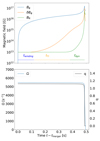Fig. 2. Top: time evolution of the magnetic field strength for a typical HMNS with thermodynamic quantities taken at t − tmerger = 0.03 s at a radius of RTI = 7 km and with an initial magnetic field strength of BR, 0 = 1013 G. Bottom: time evolution of the rotational angular velocity Ω and the shear rate q.

• (i)

  First, the shear amplifies the toroidal magnetic field. This winding phase lasts for ≃0.15 s.

• (ii)

  When the toroidal magnetic field is stronger than the critical magnetic field $B_{\varphi ,\mathrm{crit}}$, the non-axisymmetric magnetic field δB_ϕ grows due to the Tayler instability. The duration of this phase is ≃0.25 s.

• (iii)

  When δB_ϕ becomes strong enough for the non-linear induction to be relevant, the dynamo sets in and increases all the magnetic field components for the next 0.08 s. The dynamo stops when the angular momentum is transported and the HMNS core settles in a rigid rotation with a low angular velocity (see bottom panel in Fig. 2).

The saturation is reached after several hundred milliseconds. Note that we neglect the contraction of the HMNS due to neutrino cooling on this timescale. This would actually increase the shear rate as the rotation maximum shifts inside, and, for cases with high mass or soft EOS, the core of the HMNS may also collapse before the saturation.

At saturation, the toroidal, radial, and perturbed magnetic fields are equal to

$$\begin{array}{cc}\hfill B_{\varphi }^{\mathrm{sat}}& =1.6\times {10}^{17}\mathrm{G},\hfill \end{array}$$(28)

$$\begin{array}{cc}\hfill B_{\mathrm{R}}^{\mathrm{sat}}& =5.9\times {10}^{16}\mathrm{G},\hfill \end{array}$$(29)

$$\begin{array}{cc}\hfill \delta B_{\varphi }^{\mathrm{sat}}& =1.0\times {10}^{17}\mathrm{G}.\hfill \end{array}$$(30)

With the saturated toroidal magnetic field, we have $\frac{{\omega }_{\mathrm{A},\mathrm{sat}}}{\mathrm{\Omega }}=0.58$, meaning that the initial assumption of ω_A ≪ Ω is verified for most of the dynamo phase until the last rapid growth where the rotational angular velocity decreases to low values due to the magnetic torque. We compare the saturation values of the axisymmetric field B_R and B_ϕ obtained by the model to the estimated saturated magnetic field from the following formulas (Fuller et al. 2019)

$$\begin{array}{cc}\hfill B_{\varphi }^{\mathrm{F},\mathrm{sat}}& =\sqrt{4\pi \rho R_{\mathrm{TI}}^2}\mathrm{\Omega }{\left(\frac{q\mathrm{\Omega }}{N}\right)}^{1/3}\approx 2.8\times {10}^{17}\mathrm{G},\hfill \end{array}$$(31)

$$\begin{array}{cc}\hfill B_r^{\mathrm{F},\mathrm{sat}}& =\sqrt{4\pi \rho R_{\mathrm{TI}}^2}\mathrm{\Omega }{\left(\frac{q^2{\mathrm{\Omega }}^5}{N^5}\right)}^{1/3}\approx 3.3\times {10}^{17}\mathrm{G},\hfill \end{array}$$(32)

$$\begin{array}{cc}\hfill \delta B_{\varphi }^{\mathrm{F},\mathrm{sat}}& =\sqrt{4\pi \rho R_{\mathrm{TI}}^2}\mathrm{\Omega }{\left(\frac{q\mathrm{\Omega }}{N}\right)}^{2/3}\approx 3.0\times {10}^{17}\mathrm{G}.\hfill \end{array}$$(33)

These values differ from the results of our models because some of the model’s assumptions are not valid before reaching the predicted saturated values. Indeed, both Fuller’s and Spruit’s predictions give ω_A > Ω and ω_A > N with our values. These values are not reached, as the differential rotation is quenched before. Nonetheless, the saturated values still agree within a factor of 3 − 5.

It is interesting to note that the alternative model of Spruit (2002) predicts similar magnetic field strength at saturation:

$$\begin{array}{cc}\hfill B_{\varphi }^{\mathrm{S},\mathrm{sat}}& =\sqrt{4\pi \rho R_{\mathrm{TI}}^2}q\left(\frac{{\mathrm{\Omega }}^2}{N}\right)\approx 3.2\times {10}^{17}\mathrm{G}\hfill \end{array}$$(34)

$$\begin{array}{cc}\hfill B_r^{\mathrm{S},\mathrm{sat}}& =\sqrt{4\pi \rho R_{\mathrm{TI}}^2}{q}^2\left(\frac{{\mathrm{\Omega }}^4}{N^3}\right)\approx 3.9\times {10}^{17}\mathrm{G}.\hfill \end{array}$$(35)

This can be interpreted by the fact that the rotation and Brunt-Väisälä frequencies are of the same order of magnitude. Overall, with an initial magnetic field of 10¹³ G, the TS-dynamo could generate an intense dipole and an even stronger toroidal magnetic field when the long-lived HMNS survives for longer than 0.5 s after the BNS mergers.

3.2. Dependence on the initial dipole magnetic field strength

For BNS mergers, the duration of the dynamo is quite essential as it may determine the time at which the remnant collapses into a black hole. This duration is expected to depend on the initial intensity of the large-scale poloidal magnetic field, which is uncertain as discussed above. We therefore vary the initial magnetic field strength to study its influence on the dynamo. Figure 3 shows the time evolution for different initial magnetic fields B_R, 0. While the maximum magnetic field strength is similar for all cases, the time to reach saturation Δt_sat decreases drastically with the increase of the initial magnetic field strength (see Table 1).

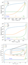Fig. 3. Time evolution of the magnetic field for different initial magnetic dipole strength BR, 0 with BR, 0 = 1014 G (top), BR, 0 = 1012 G (middle) and BR, 0 = 1010 G (bottom).

To realistically estimate the initial dipole field strength, the magnetic field in the core of the HMNS, amplified by the Kelvin-Helmholtz (KH) instability at the onset of the merger, should be explored with dissipation (Rasio & Shapiro 1999; Kiuchi et al. 2014, 2018, 2024). Due to this instability, the large-scale initial magnetic field could be amplified and potentially be stronger than B_R, 0 = 10¹³ G. Therefore, the TS dynamo could saturate in less than 0.5 s.

To complete this picture, we can estimate the duration of each phase of the dynamo process. The first phase is the winding phase, during which the toroidal field is amplified. It lasts until either the toroidal field becomes strong enough for the Tayler instability to grow as fast as B_ϕ (Barrère et al. 2022), or that it becomes strong enough to reach the critical magnetic field for the instability to start with the high viscosity. The formula for the winding time is therefore

$$\begin{array}{c}\hfill t_{\mathrm{winding}}=\frac{max({\omega }_{\mathrm{A},\mathrm{TI}},{\omega }_{\mathrm{A},\mathrm{crit}})}{q\mathrm{\Omega }{\omega }_{\mathrm{R},0}}=max({(q^2{\omega }_{\mathrm{R},0}^2\mathrm{\Omega })}^{-1/3},\frac{{\omega }_{\mathrm{A},\mathrm{crit}}}{q\mathrm{\Omega }{\omega }_{\mathrm{R},0}}),\end{array}$$(36)

where ω_A, crit and ω_R, 0 are the Alfvén frequency of the critical magnetic field due to viscosity and the initial Alfvén frequency, respectively. ω_A, TI is the Alfvén frequency when the Tayler instability becomes dynamically relevant, that is when σ_shear = σ_TI, which is given by

$$\begin{array}{c}\hfill {\omega }_{\mathrm{A},\mathrm{TI}}={\left(q{\mathrm{\Omega }}^2{\omega }_{\mathrm{R},0}\right)}^{1/3}.\end{array}$$(37)

At the end of the winding phase, the toroidal magnetic field is equal to

$$\begin{array}{c}\hfill B_{\varphi }(t_{\mathrm{winding}})=q\mathrm{\Omega }{t}_{\mathrm{winding}}{B}_{\mathrm{R},0}.\end{array}$$(38)

For the Tayler instability phase, we adapt Eq. (51) of Barrère et al. (2022) considering that B_ϕ(t_winding) is given by Eq. (38). Introducing the corresponding Alfvén frequency ω_A, winding, we find

$$\begin{array}{c}\hfill t_{\mathrm{TI}}\sim \frac{\mathrm{\Omega }}{{({\omega }_{\mathrm{A},\mathrm{winding}})}^2}ln\left(\frac{{\omega }_{\mathrm{A},\mathrm{winding}}^{2}r}{\mathrm{\Omega }\delta v_{\mathrm{A},0}}\right),\end{array}$$(39)

where δv_A, 0 = δv_A(t = 0).

Finally, we use the same formula as Barrère et al. (2022) for the dynamo phase

$$\begin{array}{c}\hfill t_{\mathrm{dyn}}={\left(\frac{B_{\varphi }}{{\partial }_t^2{B}_{\varphi }}\right)}^{1/2}=\frac{\mathrm{\Omega }}{{\omega }_{\mathrm{A},\mathrm{dyn}}^2}{\left(\frac{N}{q{\omega }_{\mathrm{A},\mathrm{dyn}}}\right)}^{1/2},\end{array}$$(40)

where ω_A, dyn = (qNΩ⁴ω_R, 0²)^1/7 is the Aflvén frequency for which the winding rate is equal to the non-linear growth rate σ_NL of the radial magnetic field B_r.

Figure 4 compares these timescale estimates to the ones measured in the one-zone model. The analytical predictions are overall in good agreement with only a slight overestimation compared to the model results. We also give a simple fit of the total dynamo time

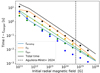Fig. 4. Timescale of the different phases post-merger of the TS dynamo as a function of the initial radial magnetic field strength. The points are measured from the one-zone model, while the lines represent analytical estimates. The vertical dashed line indicates the volume-averaged poloidal magnetic field in Aguilera-Miret et al. (2024).

$$\begin{array}{c}\hfill t_{\mathrm{total}}\approx 65.7{\left(\frac{B_{\mathrm{R},0}}{{10}^{10}}\right)}^{-0.71}\mathrm{s}.\end{array}$$(41)

This shows that the TS dynamo can grow in a few seconds as long as the initial magnetic field strength is higher than 10¹² G. This figure shows that the shear time dominates the total time for initial magnetic field strengths lower than 10¹² G. In this case, a higher rotational angular velocity or shear rate would linearly decrease the total dynamo time. For higher initial magnetic field strength, the Tayler instability phase dominates the total time, and therefore, the Tayler-instability growth rate becomes a key parameter. In the first few milliseconds after the mergers, the Kelvin-Helmholtz instability amplifies the magnetic field, which places a lower bound on the radial component of the initial large-scale magnetic field for our one-zone model. However, the strength of this lower bound remains unknown. As an initial guess, we take the volume-averaged poloidal magnetic field B_R, 0 ∼ 5 × 10¹⁴ G found in the simulations of Kelvin-Helmholtz instability with a realistic initial field (Fig. 4 of Aguilera-Miret et al. 2024). An initial magnetic field B_R, 0 ∼ 5 × 10¹⁴ G means that it is plausible that the TS dynamo saturates after ≤50 ms.

4. Comparison with a 3D GRMHD simulation

In the previous section, we showed that the TS dynamo is able to grow and reach saturation on a timescale of a few tens of milliseconds for an initial dipole higher than 10¹⁵ G, which is the typical dipole value used in GRMHD simulations of BNS mergers (e.g., Giacomazzo & Perna 2013; Kiuchi et al. 2014, 2024; Mösta et al. 2020). As a consequence, the magnetic fields would be expected to grow from the TS dynamo in such GRMHD simulations. In this section, we analyze the data of a 3D ideal GRMHD simulation in which the massive neutron star remnant is long-lived (Kiuchi et al. 2024). Since the remnant is differentially rotating during the duration of the simulation (see Figure 1), we call it an HMNS in the following. Note that it may become a supramassive neutron star once in solid body rotation or collapse to a black hole in the case of a strong spin-down.

Since we look for the TS dynamo, we focus our analysis on the core of the BNS merger remnant at radii lower than 10 km. In this region, the resolution is Δx = 12.5 m in the range [0, 4.5] km and Δx = 25 m in the range [4.5, 9] km, which is roughly the region where the positive differential rotation is found. In this region, the resolution becomes Δx = 100 m after t − t_merger = 0.050 s. The numerical techniques and the study of the other regions of these simulations are detailed in Kiuchi et al. (2024). Note that the outer surface of the merger remnant core for which q is negative is subject to the αΩ dynamo as reported in Kiuchi et al. (2024).

4.1. Dynamics of the GRMHD simulation

The 3D neutrino radiation GRMHD simulation for a BNS merger of a symmetric binary case, with masses of 1.35−1.35 M_⊙ and a stiff equation of state, DD2 (Hempel & Schaffner-Bielich 2010), shows that the merger results in a HMNS that survives for timescales > 0.15 s. The rotation profile in the equatorial plane of the HMNS shows a differential rotation with q > 0 until 10 km (see Fig. 1). This leads to the winding of the poloidal magnetic field in the core of the remnant. Figure 5 compares the time evolution of the magnetic field strength in the 3D GRMHD simulation and the one-zone model. The radial magnetic field in the one-zone model is amplified to its saturation values within 0.02 s, while in the GRMHD simulation, the radial magnetic field strength varies slightly and overall remains constant, staying close to its initial value around 10¹⁵ G. This shows that no TS dynamo processes occur in the simulation’s HMNS core even though it would be expected according to the theoretical prediction. In addition, the non-axisymmetric vertical field δB_z is only decreasing in this region, while it should be growing to a similar amplitude as the δB_ϕ of the one-zone model. In this simulation, the toroidal magnetic field quickly reaches 10¹⁷ G due to the winding around 7 km. This gives an Alfvén frequency of ω_A = 2100 s⁻¹, which is smaller but of the same order of magnitude as N ≈ 5000 s⁻¹ ∼ Ω ≈ 5500 s⁻¹. The local Alfvén frequency may even be closer to the rotation frequency, as the local field can be stronger than 10¹⁷ G.

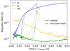Fig. 5. Time evolution of the axisymmetric magnetic field and δBz for the GRMHD simulation (solid lines) in the unstable region (see Section 2.1 and Figure 7) and for the one-zone model (dashed lines) that has been shifted temporally.

To understand why there is no TS dynamo, we look at a snapshot of the simulation in a plane at z = 2 km and t − t_merger = 0.03 s (see Fig. 6). We see that the toroidal magnetic field is amplified to a maximum value of 4 × 10¹⁷ G (top panel of Figure 6). Since this is larger than the critical magnetic field for a strong viscosity, the simulation should be unstable to the Tayler instability but the non-axisymmetric component of the radial magnetic field does not show any evidence for the Tayler instability. Indeed, its main mode is an m = 2 mode, and the geometry corresponds well to the velocity field in the equatorial plane (bottom panel of Fig. 6). The origin of this m = 2 mode is well-known and comes from the initial geometry and mass ratio of the binary. Figure 6 shows that the velocity field is not a purely m = 2 mode as the initial m = 2 mode can also degrade as a m = 1 mode, but it is different from the m = 1 mode from the Tayler instability. Indeed, the m = 2 and degraded m = 1 modes give the radial magnetic field exactly the same geometry as the radial velocity field and it has the ring shape of the toroidal field. In addition, according to simulations of the Tayler instability (Ji et al. 2023; Barrère et al. 2025), we would expect to see some opposing polarities of the radial field on a meridional slice, contrary to the geometry observed in Figure 7, which is the same as the toroidal field. Note that, in the case of an unequal mass binary neutron star merger, the m = 1 mode may be more easily triggered due to the asymmetry of the initial system.

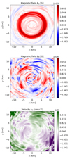Fig. 6. Snapshot of the toroidal magnetic field (top), radial magnetic field (middle) and radial velocity (bottom) in the core of the HMNS, taken in the plane z = 2 km at t − tmerger = 0.035 s.

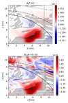Fig. 7. Snapshot of the axisymmetric toroidal magnetic field (top) and a slice of the radial magnetic field BR (bottom) in the core of the remnant neutron star at t − tmerger = 0.060 s and y = 0 km. The gray contours correspond to the regions stable to the Tayler instability according to the geometric criterion (Eq. (42) with m = 1). Density contours for ρ ∈ [1012, 1013, 1014] g cm−3 are respectively the dotted, dashed-dotted, solid black lines. The dashed green line corresponds to the peak of the rotation rate in the HMNS (see Figure 1).

Positive differential rotation can stabilize the Tayler instability, as shown by Kiuchi et al. (2011), but the toroidal magnetic field is decreasing vertically in the north hemisphere in the unstable region (see Fig. 7), which makes it unstable (see Eq. (27) of Kiuchi et al. 2011). From this criterion, the core of the remnant at t − t_merger = 0.06 s should be unstable to the Tayler instability with a fast-growing rate of σ_TI ∼ ω_A, because we are in the “slow” rotating regime.

To be unstable to the Tayler instability, the geometry of the magnetic field is also important, as the size of the magnetic field can limit the wavelength. To estimate what is the maximal wavelength available, we used the geometrical instability criterion for a wave from Goossens & Tayler (1980)

$$\begin{array}{c}\hfill \frac{B_{\varphi }^2}{4\pi R_{\mathrm{TI}}^{2}sin\theta }(m^2-2{cos}^2\theta -2sin\theta cos\theta {\partial }_{\theta }log{B}_{\varphi })<0.\end{array}$$(42)

Figure 7 shows the toroidal magnetic field with the gray contours showing where the Tayler instability is stable according to this criterion with m = 1. The magnetic field should indeed be unstable to the Tayler instability, but the unstable domain is relatively small, with a typical size of around 1 km. Contrary to the one-zone model, the hypothesis ω_A ≪ Ω is not verified in the unstable domain.

Lastly, another instability criterion is that $B_{\mathrm{R}}/B_{\varphi }<\frac{k_{\varphi }}{k_{\mathrm{R}}}$ which implies that the magnetic tension due to the radial component should not exceed the magnetic pressure due to the toroidal component (Eq. (8)) to operate the Tayler instability. This criterion is usually given for an axisymmetric B_R but it is unclear whether the magnetic tension from a non-axisymmetric B_{R, m ≠ 0} would stabilize the instability by overcoming the magnetic tension from the background toroidal field.

Looking at the middle panel of Fig. 6, this criterion may explain why the Tayler instability is temporarily stabilized as the radial length of B_R is quite small. However, after some time, B_ϕ grows in strength and size with the winding (Figure 7). At the same time, the amplitude of the non-axisymmetric modes decreases and the instability criterion becomes verified.

In any case, these non-axisymmetric modes amplify the magnetic field to a lower strength than the ones in the one-zone model and are expected to dissipate less than a hundred milliseconds after the merger as the gravitational wave luminosity decreases (Radice & Bernuzzi 2023). These modes might cause a delay in the appearance of the TS dynamo, but this does not explain why it does not appear later in the simulation.

4.2. Numerical dissipation analysis

The absence of the Tayler instability in this 3D GRMHD simulation could be due to the wavelength of the Tayler instability being lower than the grid resolution or to the fact that the numerical resistivity and viscosity reduce the growth rate of the instability. Thus, we estimate the expected wavelength of the Tayler instability if it were growing in the simulation. In ideal MHD, the wavelength would be limited by the buoyancy and would give ${\lambda }_{\mathrm{TI}}=\frac{{\omega }_{\mathrm{A}}}{N}R\approx R$ in the simulation. This wavelength is well resolved so we need to look at the impact of diffusion on the wavelength. From the instability criterion, the wavelength λ_crit = 2π/k_TI, crit below which the Tayler instability should occur is

$$\begin{array}{c}\hfill {\lambda }_{\mathrm{crit}}=\frac{2\pi R_{\mathrm{TI}}{\omega }_{\mathrm{A},\mathrm{crit}}}{N}=\{\begin{array}{cc}2\pi R_{\mathrm{TI}}{\left(\frac{\mathrm{\Omega }}{N}\right)}^{1/2}{\left(\frac{\nu }{R_{\mathrm{TI}}^2\mathrm{\Omega }}\right)}^{1/4}\hfill & \mathrm{if}{\omega }_{\mathrm{A}}\ll \mathrm{\Omega },\hfill \\ 2\pi R_{\mathrm{TI}}{\left(\frac{\nu }{R_{\mathrm{TI}}^{2}N}\right)}^{1/3}\hfill & \mathrm{if}\mathrm{\Omega }\ll {\omega }_{\mathrm{A}}.\hfill \end{array}\end{array}$$(43)

As this wavelength depends on the numerical resistivity and viscosity inside the simulation, we estimate the numerical resistivity and viscosity. We use the fitting formula derived for Eulerian MHD codes in Rembiasz et al. (2017)

$$\begin{array}{c}\hfill {\nu }_{\star }={\mathcal{R}}_{\nu }^{\mathrm{\Delta }x}\mathcal{V}\mathcal{L}{\left(\frac{\mathrm{\Delta }x}{\mathcal{L}}\right)}^r,\end{array}$$(44)

where 𝒱 and ℒ are the characteristic speed and length of the system, ℛ_ν^Δx and r are fitting parameters. We use the fitting parameters r = 4.95 and ℛ_ν^Δx = 42 for the HLLD solver with the fourth-order Runge Kutta method, as it is the same Riemann solver used in our GRMHD simulations. We use the fast magnetosonic speed for the characteristic velocity as found in the study 𝒱 = max(v_A, c_s)≈c_s ≈ 1.2 × 10¹⁰ cm s⁻¹ for the characteristic speed. We take the characteristic length as a variable ℒ = λ_crit. Since the numerical resistivity depends on the resolution and on the scale we are considering, by combining Eqs. (43) and (44), we have to solve the equation

$$\begin{array}{c}\hfill \{\begin{array}{cc}{\lambda }_{\mathrm{crit}}^{1.9875}=2\pi R_{\mathrm{TI}}{\left(\frac{\mathrm{\Omega }}{N}\right)}^{1/2}{\left(\frac{{\mathcal{R}}_{\nu }^{\mathrm{\Delta }x}\mathcal{V}\mathrm{\Delta }{x}^{4.95}}{R_{\mathrm{TI}}^2\mathrm{\Omega }}\right)}^{1/4},\hfill & \mathrm{if}{\omega }_A\ll \mathrm{\Omega },\hfill \\ {\lambda }_{\mathrm{crit}}^{2.317}=2\pi {\left(\frac{{\mathcal{R}}_{\nu }^{\mathrm{\Delta }x}\mathcal{V}\mathrm{\Delta }{x}^{4.95}{R}_{\mathrm{TI}}}{N}\right)}^{1/3},\hfill & \mathrm{if}{\omega }_A\gg \mathrm{\Omega },\hfill \end{array}\end{array}$$(45)

which, with Δx = 100 m, gives λ_crit = 1.55 km. Note that, in the fast-rotating limit (ω_A ≪ Ω), we get λ_crit = 2.4 km at a R_TI = 7 km. In the case where the geometry does not constrain the wavelength, the Tayler instability would be resolved by a hundred-meter resolution.

However, the unstable region of the magnetic field is limited by its vertical length ≈1 km (Figure 7), and we therefore have to limit the wavelength of the Tayler instability. To check the impact of dissipation on a mode with a 1 km wavelength, we solve the local dispersion relation of Acheson & Gibbons (1978) with equal diffusivities, ν = η = κ. We also assume the magnetic field to be increasing with radius and decreasing vertically, and we take the other quantities to be the same as in the simulation (see Appendix C for more details). Figure 8 shows that the growth rate in the limit of low dissipation is in fair agreement with σ_TI ≈ ω_A, which is consistent with the regime ω_A ≫ Ω. The stability limit due to dissipation is found to be in good agreement with the criterion ω_A = k_TI²η (dashed line in Fig. 8). We also note that even for a high dissipation like the neutrino viscosity ν_HMNS = 7.36 × 10⁷ cm² s⁻¹, the growth rate is unchanged compared to the ideal MHD case. We would therefore expect the instability to grow in the absence of numerical limitations.

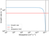Fig. 8. Growth rate of the Tayler instability as a function of dissipation, with ν = η = κ. The red line shows the theoretical growth rate in the regime of Ω ≪ ωA. The dashed line is the stabilizing limit given by kTI2η = ωA.

We thus use the limit given by Eq. (20) with the numerical dissipation as the criterion to see whether the Tayler instability can develop in the numerical simulation. Figure 9 shows the critical magnetic field for the numerical viscosity and resistivity in the code depending on the length scale below 1 km for different resolutions. The magnetic field found in the simulation is close to the critical magnetic field with the estimated dissipation of a 100-meter resolution, which may explain why the simulation is stable to Tayler instability at this resolution. Overall, in our understanding, the Tayler instability may be stabilized by the non-axisymmetric modes initially and later on by the resolution that is not enough to resolve the small region where it should be unstable.

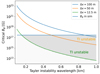Fig. 9. Critical magnetic field $B_{\varphi ,\mathrm{crit}}$ (Eq. (20)) in the numerical simulation depending on the wavelength of the Tayler instability for several resolutions with the numerical viscosity and resistivity estimated with the simulation grid size (Eq. (44)). The Tayler instability should be unstable in the simulation when the critical field is weaker than the magnetic field in the GRMHD simulation (gray region for Δx = 12.5 m).

5. Discussion

5.1. Comparison with Boussinesq simulations

Like the one-zone model of Barrère et al. (2022), the model of this article relies on strong assumptions to overcome the non-linearity of the dynamo mechanism, especially for the saturation phase (Spruit 2002; Zahn et al. 2007; Fuller et al. 2019). A comparison with the recent 3D numerical simulations of the TS dynamo with a positive differential rotation (Barrère et al. 2023, 2025) is therefore useful to test the validity of these necessary assumptions. Their simulations show the existence of several TS dynamo branches, but we only consider the strong, dipolar branch, which has been thoroughly studied by Barrère et al. (2025) and harbours the strongest magnetic fields. Furthermore, this solution is in good agreement with the scaling laws in Eqs. (31)–(33), derived by Fuller et al. (2019), which correspond to the formalism used in our one-zone model, with, however, a normalization factor significantly lower than 1.

In the region of the HMNS core with a positive shear (5 − 10 km), the stratification is in the range N/Ω ≈ 0.5 − 1, which is covered by the investigation of Barrère et al. (2025). By using the parameters of a typical HMNS (R = 7 km, ρ = 3.7 × 10¹⁴ g cm⁻³, and Ω = 5468 s⁻¹) and extrapolating to q ∼ 1, we infer from the numerical models of Barrère et al. (2025) with N/Ω = 0.5 and N/Ω = 1 that the axisymmetric toroidal, poloidal magnetic fields and the magnetic dipole should reach

$$\begin{array}{cc}\hfill B_{\mathrm{tor}}^{m=0}& \approx 0.63-1.4\times {10}^{16}\mathrm{G},\hfill \end{array}$$(46)

$$\begin{array}{cc}\hfill B_{\mathrm{pol}}^{m=0}& \approx 0.15-1.5\times {10}^{15}\mathrm{G},\hfill \end{array}$$(47)

$$\begin{array}{cc}\hfill B_{\mathrm{dip}}& \approx 0.79-6.3\times {10}^{14}\mathrm{G},\hfill \end{array}$$(48)

respectively. The axisymmetric toroidal magnetic field $B_{\mathrm{tor}}^{m=0}$ is therefore weaker by a factor of ∼20 − 45 than $B_{\varphi }^{\mathrm{F},\mathrm{sat}}$ (Eq. (31)). Likewise, the magnetic fields $B_{\mathrm{tor}}^{m=0}$ and B_dip are ∼220 − 4200 times weaker than B_r^F, sat (Eq. (32)), which is consistent with the fact that the TS dynamo in the simulations of Barrère et al. (2025) produces weaker large-scale magnetic fields than predicted by the formalism of Fuller et al. (2019). These intensities predicted by the scaling of MHD simulations are much lower than the one-zone model predicts.

These lower intensities are already reached in the GRMHD simulation we present in this study due to the high initial poloidal magnetic field. This can be interpreted in two different ways. First, we assume that the MHD simulation saturation gives the upper limit of the magnetic field in the GRMHD simulation. This means that, if the Tayler-Spruit dynamo were active in the GRMHD simulation, it would lead to a decrease in the magnetic field until it reaches the MHD saturation values, an evolution we do not see. In this case, the Tayler-Spruit dynamo would dissipate the axisymmetric toroidal magnetic field and prevent its growth to values ≥2 × 10¹⁷ G. The second interpretation could be that the saturation intensities are different due to setup differences, as the background profiles, the differential rotation, and how it is generated in the MHD simulations could be quite important for the saturation values.

Moreover, these MHD simulations are likely to underestimate the magnetic field strength in a realistic HMNS. Indeed, for computational reasons, the simulations were run with much higher resistivities than realistic estimates, which hinders the dynamo process. Moreover, the quantities $B_{\mathrm{tor}}^{m=0}$, $B_{\mathrm{pol}}^{m=0}$, and B_dip are volume-averaged. This suggests that the magnetic fields must be stronger locally when they are concentrated in some regions of the integration domain, which happens when the stratification increases.

5.2. MRI-driven dynamo vs TS dynamo

As it is argued in Margalit et al. (2022), the TS dynamo could also be relevant for the transport of angular momentum where the differential rotation is decreasing with radius. However, depending on the Brunt-Väisälä frequency, this region would be unstable to the MRI, which has a much faster growth rate than the TS dynamo in the fast-rotating case. For this reason, the MRI is expected to saturate first, and the Tayler instability would not impact this region. To confirm this picture, we compute the growth rate of both instabilities in the equatorial plane at r = 20 km with a magnetic field B₀ = 10¹⁵ G as it is found after the Kelvin-Helmholtz instability. We obtain

$$\begin{array}{cc}\hfill {\sigma }_{\mathrm{MRI}}& =\frac{q\mathrm{\Omega }}{2}\approx 2600{\mathrm{s}}^{-1}\hfill \\ \hfill {\sigma }_{\mathrm{TS}}& =\frac{{\omega }_{\mathrm{A}}^2}{\mathrm{\Omega }}\approx 0.072{\left(\frac{B_0}{{10}^{15}\mathrm{G}}\right)}^2{\mathrm{s}}^{-1}\ll {\sigma }_{\mathrm{MRI}},\hfill \end{array}$$(49)

due to ω_A ≪ Ω. Interactions from the turbulence developed by the MRI and the TS dynamo would occur at the radius where the differential rotation changes sign, making this transition region difficult to study.

5.3. Angular momentum transport and spin-down time

To have the complete picture of the angular momentum transport in the HMNS, we first describe the transport in the outer region, R ≳ 10 km, which is unstable to the MRI. The angular momentum transport timescale due to MRI turbulence is

$$\begin{array}{c}\hfill t_{\mathrm{MRI}}\approx \frac{R^2}{{\alpha }_{\mathrm{turb}}H\mathrm{\Omega }}\sim 5\times {10}^{-3}{\left(\frac{{\alpha }_{\mathrm{turb}}}{0.1}\right)}^{-1}{\left(\frac{\mathrm{\Omega }}{{\mathrm{\Omega }}_K}\right)}^{-1}{\left(\frac{H}{R/3}\right)}^{-2}[\mathrm{s}].\end{array}$$(50)

The spin-down in the outer region would be from the magnetic torque of the large-scale magnetic field generated by the αΩ dynamo. On the other hand, our study shows that in the inner core, the angular momentum transport timescale due to the TS dynamo corresponds to the time it takes to reach saturation. Indeed, the very large saturated magnetic fields lead to very fast transport of angular momentum on a much shorter timescale than the dynamo growth timescale. This growth lies in the range 10⁻² − 10² s and scales with the initial magnetic field as $t_{\mathrm{total}}=65.7{\left(\frac{B_{\mathrm{R},0}}{{10}^{10}}\right)}^{-0.71}$ s. One interesting feature is that due to the positive differential rotation, the angular momentum would be transported inwards rather than outwards.

The spin-down time depends on how we consider the generated magnetic field inside the remnant. We first consider that the magnetic field stays buried in the core of the HMNS, then it would act as a torque and slow the core down following Eq. (5). By taking the saturated magnetic field values of the one-zone model (Eqs. 28 and 29), the core would slow down at a rate of

$$\begin{array}{c}\hfill {\gamma }_{\mathrm{spin}-\mathrm{down},\mathrm{core}}\equiv \frac{\dot{\mathrm{\Omega }}}{\mathrm{\Omega }}=-\frac{R_{\mathrm{TI}}^3{B}_{\mathrm{R}}{B}_{\varphi }}{I\mathrm{\Omega }}\approx 3.5\times {10}^2{\mathrm{s}}^{-1}.\end{array}$$(51)

We can also assume that the obtained dipole becomes the dipole at the surface of a remnant neutron star without matter outside. Then, the dipole formula gives the following spin-down rate of

$$\begin{array}{c}\hfill {\gamma }_{\mathrm{spin}-\mathrm{down},\mathrm{dipole}}\equiv \frac{\dot{\mathrm{\Omega }}}{\mathrm{\Omega }}=-\frac{B_r^2{R}_{\mathrm{TI}}^6{\mathrm{\Omega }}^2}{6c^{3}I}\approx 4.5\times {10}^{-2}{\mathrm{s}}^{-1}\end{array}$$(52)

assuming that the saturated value of the dipole is B_r ∼ B_R = 4 × 10¹⁶ G. The spin-down due to the magnetic torque would therefore be faster than the dipole spin-down and slow the remnant down on a timescale of milliseconds.

Hence, the remnant would collapse in a few milliseconds when the dynamo saturates and the rotational kinetic energy would not be emitted in electromagnetic waves. If the magnetic braking follows the torque used in this study, this could therefore shorten the lifetime of a remnant neutron star after the merger depending on the initial radial field B_R, 0. However, if we consider the saturated values from Barrère et al. (2025), the spin-down value due to the magnetic torque would be a thousand times slower γ_{spin − down, core} ≈ 0.33 s⁻¹. The collapse time would then be around O(1) s after the dynamo saturation rather than O(0.010) s.

6. Conclusions

We have investigated the TS dynamo in the context of BNS mergers. Following Barrère et al. (2022), we developed a one-zone model of the TS dynamo for a BNS merger remnant with realistic parameters estimated from a 3D GRMHD simulation.

We found that the TS dynamo could develop in the core of remnant neutron stars due to its positive differential rotation. Due to the impact of neutrino viscosity, the toroidal magnetic field must be amplified to higher values than 3.2 × 10¹⁵ G by the winding in order to be Tayler-unstable.

The magnetic field’s evolution can be divided into three phases: the winding phase, the Tayler instability phase and the non-linear growth of the dynamo. Saturation occurs when the differential rotation is effectively quenched by the Maxwell stress. The magnetic field generated by the dynamo saturates at a very high intensity of B_ϕ = 1.6 × 10¹⁷ G and B_R = 5.9 × 10¹⁶ G for the magnetic dipole, according to the one-zone model. These strong intensities must be taken with caution as current simulations of the TS dynamo applied to PNSs predict a weaker toroidal field of 10¹⁶ G and a poloidal field of 10¹⁵ G.

The saturated magnetic field strength does not depend on the initial magnetic field, unlike the time required to reach saturation, which can range from 0.1 s for a magnetic dipole of 10¹⁴ G to 2.4 s for a magnetic dipole of 10¹² G, which becomes comparable to the O(1) s, which corresponds to the HMNS lifetime in the long-lived case. In the first case, the transport of angular momentum by the TS dynamo would lead to a faster collapse to a black hole or a faster spin-down of the remnant. This shows that the TS dynamo would be important in the case of a long-lived remnant neutron star as long as the initial magnetic field dipole is higher than 10¹² G.

However, these results depend on whether the TS dynamo grows fast enough, and consequently on the resulting magnetic dipole after the Kelvin-Helmholtz instability. Using the study of Aguilera-Miret et al. (2024), we estimate the large-scale poloidal magnetic field to be of the order of the volume-averaged magnetic field 5 × 10¹⁴ G, and the dynamo would saturate in less than 50 milliseconds. This would transport the angular momentum very efficiently in long-lived remnants and potentially reduce their lifetime, depending on the magnetic spin-down mechanism. Nonetheless, the volume-averaged magnetic field is different from the large-scale magnetic field. A more detailed study is therefore needed, and it would require to use realistic initial magnetic fields in the neutron stars and preferentially have a converged growth of the Kelvin-Helmholtz instability.

As we discussed in Section 5.1, the simulations by Barrère et al. (2025) give weaker saturated magnetic field strengths than our results but the differences could be due to a cylindrical rotation profile and the different background stratification. The value of the magnetic dipole needs to be confirmed by 3D numerical simulation with a rotation profile and a background stratification corresponding to a remnant neutron star. This is left to a further study, which should also address the question of the interaction between the TS dynamo and the MRI instability that operates at cylindrical radii larger than 10 km.

The TS dynamo operating in the remnant neutron star could have significant consequences for astrophysical observations. First, the angular momentum transport and the magnetic braking would happen when the dynamo saturates, which would lead to the collapse of the remnant neutron star if it is more massive than the maximum mass of a non-rotating neutron star M_TOV. Otherwise, it would lead to a stable, slow-rotating neutron star with a strong magnetic field, a proto-magnetar. If the rotation is damped as fast as described by the magnetic torque of the saturated field, the lifetime of the remnant neutron star would be reduced and could prevent the late-time emission of a fast-rotating proto-magnetar. These results, in particular the rate of magnetic braking, need to be tested with numerical simulations.

In addition, having motions due to the TS dynamo in the neutron star remnant is expected to lead to some emission in gravitational waves, which might be detectable for a close event. Using Fuller’s formalism, we estimate the amplitude of the velocity perturbations due to TS dynamo with the formula

$$\begin{array}{c}\hfill \delta v_{r,\mathrm{sat}}=\delta v_{\mathrm{A},\mathrm{sat}}\frac{{\omega }_{\mathrm{A},\mathrm{sat}}^2}{N\mathrm{\Omega }}\approx 4.5\times {10}^9\mathrm{cm}{\mathrm{s}}^{-1}.\end{array}$$(53)

For the sake of simplicity, we estimate the strain by using the order of magnitude derived from the quadrupole formula (Kokkotas 2002)

$$\begin{array}{c}\hfill h\approx \frac{G}{c^4}\frac{\epsilon E_{\mathrm{turb}}}{D_{\mathrm{GW}}},\end{array}$$(54)

where ε is the efficiency to convert the turbulent energy to gravitational waves that we assume to be low, with ε ≈ 5%. The kinetic energy is computed by assuming that this velocity is constant in the region from 5 to 10 km and oscillates at the Brunt-Väisälä frequency N. A distance of 100 Mpc would then give a strain of h ≈ 2 × 10⁻²⁵, which is of the same order but slightly lower than the sensitivity of the future generation of gravitational detectors. Knowing that the kinetic energy predicted here can be viewed as optimistic, a direct detection of the signal will be difficult but the TS dynamo would still impact the collapse time of the remnant. Further investigations of the TS dynamo in BNS mergers are therefore important to better understand future multi-messenger observations.

Acknowledgments

This work was supported by the European Research Council (MagBURST grant 715368) and by the “Action thématique Phénomènes Extrêmes et Multi-messagers” (AT-PEM) of CNRS/INSU PN Astro with INP and IN2P3, co-funded by CEA and CNES. This work was in part supported by the Grant-in-Aid for Scientific Research (grant Nos. 23H04900, 23H01172, 23K25869) of Japan MEXT/JSPS.

References

Appendix A: Effects from general relativity

In the context of BNS merger remnant neutron stars, effects from general relativity can become important and the formalism needs to be adapted to a 3+1 decomposition. The three-component velocity vⁱ, which corresponds to the Newtonian velocity in the non-relativistic limit, is defined by

$$\begin{array}{c}\hfill v^i=\frac{u^i}{u^t},\end{array}$$(A.1)

where u^μ is the four-component velocity, u^t, u^j being its time and space components. In our simulation, the shift vector can be neglected at radii larger than 5 km. We can also assume that the movement of the flow is non-relativistic meaning that u^t = W/α ≈ 1/α, where W is the Lorentz factor of the flow.

In ideal GRMHD, the induction equation is the same as the Newtonian case but for the magnetic field in the inertial frame ℬⁱ, written as B_i in the following, and the three-component velocity vⁱ. The magnetic field that enters the momentum equation is the magnetic field comoving with the fluid flow b^μ and the spatial components are defined as

$$\begin{array}{c}\hfill b_i=\frac{1}{\alpha u^t}(B_i+u_i\left(B^j{u}_j\right)).\end{array}$$(A.2)

Knowing that $u_{\varphi }\sim \frac{1}{\alpha }{v}_{\varphi }$ would be dominant the component of the velocity and that v_ϕ is of the order of magnitude 0.1c, the order of magnitude of the corrections would be 4% for b_ϕ as it would scale as u_ϕ² and lower for the other components. Another correction would be in the expression of the angular momentum transport by the Maxwell stress tensor which is then given by

$$\begin{array}{c}\hfill T_{R\varphi }^{\mathit{MAX}}=b^2{u}_R{u}_{\varphi }-b_R{b}_{\varphi },\end{array}$$(A.3)

where $b^2=b^{\mu }{b}_{\mu }=\frac{1}{{\alpha }^2{(u^t)}^2}(B^2+{(B^i{u}_i)}^2)$. The corrections would be of the order of $\frac{b_{\varphi }}{b_R}{u}_R{u}_{\varphi }$ and therefore around ∼8% as b_ϕ/b_R ∼ 2.

In GRMHD, the definition of the Alfvén velocity also changes to

$$\begin{array}{c}\hfill v_A^2=\frac{b^2}{4\pi \rho h+b^2},\end{array}$$(A.4)

where h is the specific enthalpy. In the case of b² ≪ 4πρh, the formalism can be simply adapted by replacing ρ by ρh. This assumption corresponds to v_A ≪ c, which holds already in the case of ω_A ≪ Ω as the rotational velocity R_TIΩ is lower than c. This correction would reduce the Alfvén frequency and thus the growth rate σ_TI by h(R_TI)∼1.126c² in the case of fast rotation.

Appendix B: Force balance at high viscosiy

Fuller et al. (2019) make the assumption of a Coriolis-Lorentz force balance for the perturbed velocity. However, another balance of the viscous forces and Lorentz force could be possible. To compare the Coriolis force and the viscous force, a local Ekman number can be defined as

$$\begin{array}{c}\hfill E=\frac{\nu k_{\mathrm{TI}}^2}{\mathrm{\Omega }},\end{array}$$(B.1)

where k_TI is the wavenumber of the displacements due to the Tayler instability. When E < 1, the Coriolis force is stronger than the viscous forces and a magnetostrophic balance can be safely assumed.

The Ekman number based on the conservative critical magnetic field $B_{\varphi ,\mathrm{crit}}$ (Eq. (20)) and its wavelength (Eq. (22)) is E ≈ 1.6 × 10⁻⁶ ≪ 1, so we can safely assume the magnetostrophic balance. From Eq. (18), we can estimate the range of magnetic fields where viscosity dominates over Coriolis force, corresponding to the regime E > 1, which is given by

$$\begin{array}{c}\hfill B_{\varphi }<B_{\varphi ,\min ,\mathrm{visc}}=\sqrt{4\pi \rho }N\sqrt{\frac{\nu }{\mathrm{\Omega }}}\approx 2.9\times {10}^{13}\mathrm{G}.\end{array}$$(B.2)

Therefore, the magnetostrophic balance can be assumed for both the Tayler instability and the dynamo phases, but not necessarily for the initial stages of the time evolution. However, the magnetic field strength is amplified to values greater than B_min, visc by the winding, for which the magnetostrophic balance can also be assumed. Since we have $B_{\varphi ,\min ,\mathrm{visc}}<B_{\varphi ,\mathrm{crit}}$, the magnetostrophic balance can be assumed during the Tayler instability phase and dynamo phase. However, in the winding phase, B_ϕ could be smaller than $B_{\varphi ,\min ,\mathrm{visc}}$ depending on the initial value of B_r. In such a case, a viscous-Lorentz force balance should be assumed. However, as this phase is not very important for the growth of the perturbed magnetic field and, therefore, we can assume a magnetostrophic balance for the whole duration. The viscous-Lorentz balance can be written as δv_⊥ ∼ δv_Aω_A/(νk_TI²), which is derived from the magnetostrophic balance δv_⊥ ∼ δv_Aω_A/Ω divided by the Ekman number. The magnetostrophic balance is used to derive the non-linear growth rate of the TS dynamo, and the balance needs to be divided by the Ekman number E with the viscous-Lorentz. In case we wanted to adapt Eq. (27), the growth rate of B_R would then be divided by E if E > 1, which gives

$$\begin{array}{cc}\hfill {\partial }_t{B}_R=({\sigma }_{\mathrm{NL}}-{\gamma }_{\mathrm{diss}})B_R& ={\mathcal{B}}_{\mathrm{TI}}\frac{{\omega }_{\mathrm{A}}^2}{N\mathrm{\Omega }}\frac{\delta B_{\perp }^2}{\max (1,E)\sqrt{4\pi \rho R_{\mathrm{TI}}^2}}\hfill \\ \hfill & -\frac{{\omega }_{\mathrm{A}}^2}{\mathrm{\Omega }}{\left(\frac{\delta B_{\perp }}{B_{\varphi }}\right)}^2{B}_R.\hfill \end{array}$$(B.3)

Appendix C: Linear study of Tayler instability

We solve the dispersion relation of Acheson & Gibbons (1978) with Python. We first use symPy to calculate the polynomial coefficients from the relation and then solve the roots of the polynomial numerically. We tested that we recover the dispersion relation in both the non-rotating ideal case and the rotating case as in Kiuchi et al. (2011). We can recover the theoretical growth rate in the two opposite limits ω_A ≪ Ω and Ω ≪ ω_A. The code used to solve the linear dispersion relation is publicly available at the address in the footnote ².

All Tables

All Figures

	Fig. 1. Top: Azimuthal averaged rotation profile of the remnant HMNS from the 3D GRMHD simulation as a function of the cylindrical radius, at different times t and vertical position z. Bottom: Averaged Brunt-Väisälä frequency of the remnant in the TS-unstable region as a function of the cylindrical radius, at different times t and different θ angles.
In the text

	Fig. 2. Top: time evolution of the magnetic field strength for a typical HMNS with thermodynamic quantities taken at t − tmerger = 0.03 s at a radius of RTI = 7 km and with an initial magnetic field strength of BR, 0 = 1013 G. Bottom: time evolution of the rotational angular velocity Ω and the shear rate q.
In the text

	Fig. 3. Time evolution of the magnetic field for different initial magnetic dipole strength BR, 0 with BR, 0 = 1014 G (top), BR, 0 = 1012 G (middle) and BR, 0 = 1010 G (bottom).
In the text

	Fig. 4. Timescale of the different phases post-merger of the TS dynamo as a function of the initial radial magnetic field strength. The points are measured from the one-zone model, while the lines represent analytical estimates. The vertical dashed line indicates the volume-averaged poloidal magnetic field in Aguilera-Miret et al. (2024).
In the text

	Fig. 5. Time evolution of the axisymmetric magnetic field and δBz for the GRMHD simulation (solid lines) in the unstable region (see Section 2.1 and Figure 7) and for the one-zone model (dashed lines) that has been shifted temporally.
In the text

	Fig. 6. Snapshot of the toroidal magnetic field (top), radial magnetic field (middle) and radial velocity (bottom) in the core of the HMNS, taken in the plane z = 2 km at t − tmerger = 0.035 s.
In the text

Fig. 7. Snapshot of the axisymmetric toroidal magnetic field (top) and a slice of the radial magnetic field BR (bottom) in the core of the remnant neutron star at t − tmerger = 0.060 s and y = 0 km. The gray contours correspond to the regions stable to the Tayler instability according to the geometric criterion (Eq. (42) with m = 1). Density contours for ρ ∈ [1012, 1013, 1014] g cm−3 are respectively the dotted, dashed-dotted, solid black lines. The dashed green line corresponds to the peak of the rotation rate in the HMNS (see Figure 1).

In the text

	Fig. 8. Growth rate of the Tayler instability as a function of dissipation, with ν = η = κ. The red line shows the theoretical growth rate in the regime of Ω ≪ ωA. The dashed line is the stabilizing limit given by kTI2η = ωA.
In the text

Fig. 9. Critical magnetic field $B_{\varphi ,\mathrm{crit}}$ (Eq. (20)) in the numerical simulation depending on the wavelength of the Tayler instability for several resolutions with the numerical viscosity and resistivity estimated with the simulation grid size (Eq. (44)). The Tayler instability should be unstable in the simulation when the critical field is weaker than the magnetic field in the GRMHD simulation (gray region for Δx = 12.5 m).

In the text

References

- Abbott, B. P., Abbott, R., Abbott, T. D., et al. 2017, ApJ, 848, L13 [CrossRef] [Google Scholar]
- Acheson, D. J., & Gibbons, M. P. 1978, Phil. Trans. R. Soc. London Ser. A, 289, 459 [CrossRef] [Google Scholar]
- Aguilera-Miret, R., Palenzuela, C., Carrasco, F., Rosswog, S., & Viganò, D. 2024, Phys. Rev. D, 110, 083014 [Google Scholar]
- Barrère, P., Guilet, J., Reboul-Salze, A., Raynaud, R., & Janka, H. T. 2022, A&A, 668, A79 [NASA ADS] [CrossRef] [EDP Sciences] [Google Scholar]
- Barrère, P., Guilet, J., Raynaud, R., & Reboul-Salze, A. 2023, MNRAS, 526, L88 [CrossRef] [Google Scholar]
- Barrère, P., Guilet, J., Raynaud, R., & Reboul-Salze, A. 2025, A&A, 695, A183 [NASA ADS] [CrossRef] [EDP Sciences] [Google Scholar]
- Baumgarte, T. W., Shapiro, S. L., & Shibata, M. 2000, ApJ, 528, L29 [NASA ADS] [CrossRef] [Google Scholar]
- Bonanno, A., Guerrero, G., & Del Sordo, F. 2020, Mem. Soc. Astron. It., 91, 249 [Google Scholar]
- Breu, C., & Rezzolla, L. 2016, MNRAS, 459, 646 [NASA ADS] [CrossRef] [Google Scholar]
- Bucciantini, N., Metzger, B. D., Thompson, T. A., & Quataert, E. 2012, MNRAS, 419, 1537 [NASA ADS] [CrossRef] [Google Scholar]
- Combi, L., & Siegel, D. M. 2023, Phys. Rev. Lett., 131, 231402 [Google Scholar]
- Cook, G. B., Shapiro, S. L., & Teukolsky, S. A. 1994a, ApJ, 424, 823 [CrossRef] [Google Scholar]
- Cook, G. B., Shapiro, S. L., & Teukolsky, S. A. 1994b, ApJ, 422, 227 [CrossRef] [Google Scholar]
- Daniel, F., Petitdemange, L., & Gissinger, C. 2023, Phys. Rev. Fluids, 8, 123701 [NASA ADS] [CrossRef] [Google Scholar]
- Denissenkov, P. A., & Pinsonneault, M. 2007, ApJ, 655, 1157 [Google Scholar]
- Duez, M. D., Liu, Y. T., Shapiro, S. L., Shibata, M., & Stephens, B. C. 2006, Phys. Rev. Lett., 96, 031101 [Google Scholar]
- Fuller, J., Piro, A. L., & Jermyn, A. S. 2019, MNRAS, 485, 3661 [NASA ADS] [Google Scholar]
- Gao, H., Ding, X., Wu, X.-F., Zhang, B., & Dai, Z.-G. 2013, ApJ, 771, 86 [Google Scholar]
- Giacomazzo, B., & Perna, R. 2013, ApJ, 771, L26 [NASA ADS] [CrossRef] [Google Scholar]
- Gompertz, B. P., O’Brien, P. T., & Wynn, G. A. 2014, MNRAS, 438, 240 [NASA ADS] [CrossRef] [Google Scholar]
- Goossens, M., & Tayler, R. J. 1980, MNRAS, 193, 833 [NASA ADS] [Google Scholar]
- Guilet, J., Müller, E., & Janka, H.-T. 2015, MNRAS, 447, 3992 [NASA ADS] [CrossRef] [Google Scholar]
- Hempel, M., & Schaffner-Bielich, J. 2010, Nucl. Phys. A, 837, 210 [Google Scholar]
- Ji, S., Fuller, J., & Lecoanet, D. 2023, MNRAS, 521, 5372 [NASA ADS] [CrossRef] [Google Scholar]
- Jouve, L., Lignières, F., & Gaurat, M. 2020, A&A, 641, A13 [EDP Sciences] [Google Scholar]
- Kastaun, W., Ciolfi, R., & Giacomazzo, B. 2016, Phys. Rev. D, 94, 044060 [Google Scholar]
- Kastaun, W., Ciolfi, R., Endrizzi, A., & Giacomazzo, B. 2017, Phys. Rev. D, 96, 043019 [NASA ADS] [CrossRef] [Google Scholar]
- Keil, W., Janka, H. T., & Mueller, E. 1996, ApJ, 473, L111 [NASA ADS] [CrossRef] [Google Scholar]
- Kiuchi, K., Yoshida, S., & Shibata, M. 2011, A&A, 532, A30 [NASA ADS] [CrossRef] [EDP Sciences] [Google Scholar]
- Kiuchi, K., Kyutoku, K., Sekiguchi, Y., Shibata, M., & Wada, T. 2014, Phys. Rev. D, 90, 041502 [Google Scholar]
- Kiuchi, K., Cerdá-Durán, P., Kyutoku, K., Sekiguchi, Y., & Shibata, M. 2015, Phys. Rev. D, 92, 124034 [NASA ADS] [CrossRef] [Google Scholar]
- Kiuchi, K., Kyutoku, K., Sekiguchi, Y., & Shibata, M. 2018, Phys. Rev. D, 97, 124039 [NASA ADS] [CrossRef] [Google Scholar]
- Kiuchi, K., Reboul-Salze, A., Shibata, M., & Sekiguchi, Y. 2024, Nat. Astron., 8, 298 [Google Scholar]
- Kokkotas, K. 2002, Gravitational wave Physics, https://phas.ubc.ca/ halpern/403/references/GW_Physics.pdf [Google Scholar]
- Lasota, J.-P., Haensel, P., & Abramowicz, M. A. 1996, ApJ, 456, 300 [Google Scholar]
- Margalit, B., Jermyn, A. S., Metzger, B. D., Roberts, L. F., & Quataert, E. 2022, ApJ, 939, 51 [NASA ADS] [CrossRef] [Google Scholar]
- Metzger, B. D., & Piro, A. L. 2014, MNRAS, 439, 3916 [NASA ADS] [CrossRef] [Google Scholar]
- Metzger, B. D., Quataert, E., & Thompson, T. A. 2008, MNRAS, 385, 1455 [CrossRef] [Google Scholar]
- Mösta, P., Radice, D., Haas, R., Schnetter, E., & Bernuzzi, S. 2020, ApJ, 901, L37 [CrossRef] [Google Scholar]
- Müller, B., Janka, H.-T., & Marek, A. 2013, ApJ, 766, 43 [CrossRef] [Google Scholar]
- Musolino, C., Ecker, C., & Rezzolla, L. 2024, ApJ, 962, 61 [NASA ADS] [CrossRef] [Google Scholar]
- Petitdemange, L., Marcotte, F., & Gissinger, C. 2023, Science, 379, 300 [NASA ADS] [CrossRef] [Google Scholar]
- Petitdemange, L., Marcotte, F., Gissinger, C., & Daniel, F. 2024, A&A, 681, A75 [NASA ADS] [CrossRef] [EDP Sciences] [Google Scholar]
- Pitts, E., & Tayler, R. J. 1985, MNRAS, 216, 139 [NASA ADS] [CrossRef] [Google Scholar]
- Price, D. J., & Rosswog, S. 2006, Science, 312, 719 [NASA ADS] [CrossRef] [Google Scholar]
- Radice, D., & Bernuzzi, S. 2023, ApJ, 959, 46 [NASA ADS] [CrossRef] [Google Scholar]
- Rasio, F. A., & Shapiro, S. L. 1999, Class. Quant. Grav., 16, R1 [Google Scholar]
- Raynaud, R., Guilet, J., Janka, H.-T., & Gastine, T. 2020, Sci. Adv., 6, eaay2732 [NASA ADS] [CrossRef] [Google Scholar]
- Reboul-Salze, A., Guilet, J., Raynaud, R., & Bugli, M. 2022, A&A, 667, A94 [NASA ADS] [CrossRef] [EDP Sciences] [Google Scholar]
- Rembiasz, T., Obergaulinger, M., Cerdá-Durán, P., Aloy, M.-Á., & Müller, E. 2017, ApJS, 230, 18 [Google Scholar]
- Rüdiger, G., & Kitchatinov, L. L. 2010, Geophys. Astrophys. Fluid Dyn., 104, 273 [CrossRef] [Google Scholar]
- Sarin, N., Omand, C. M. B., Margalit, B., & Jones, D. I. 2022, MNRAS, 516, 4949 [Google Scholar]
- Shibata, M., & Taniguchi, K. 2006, Phys. Rev. D, 73, 064027 [Google Scholar]
- Shibata, M., Duez, M. D., Liu, Y. T., Shapiro, S. L., & Stephens, B. C. 2006, Phys. Rev. Lett., 96, 031102 [Google Scholar]
- Shibata, M., Fujibayashi, S., & Sekiguchi, Y. 2021, Phys. Rev. D, 104, 063026 [NASA ADS] [CrossRef] [Google Scholar]
- Skoutnev, V. A., & Beloborodov, A. M. 2024, ApJ, 974, 290 [NASA ADS] [CrossRef] [Google Scholar]
- Spruit, H. C. 2002, A&A, 381, 923 [CrossRef] [EDP Sciences] [Google Scholar]
- Szklarski, J., & Arlt, R. 2013, A&A, 550, A94 [NASA ADS] [CrossRef] [EDP Sciences] [Google Scholar]
- Tayler, R. J. 1973, MNRAS, 161, 365 [CrossRef] [Google Scholar]
- Thompson, C., & Duncan, R. C. 1993, ApJ, 408, 194 [NASA ADS] [CrossRef] [Google Scholar]
- Zahn, J. P., Brun, A. S., & Mathis, S. 2007, A&A, 474, 145 [NASA ADS] [CrossRef] [EDP Sciences] [Google Scholar]