| Issue |
A&A
Volume 694, February 2025
|
|
|---|---|---|
| Article Number | A256 | |
| Number of page(s) | 5 | |
| Section | Cosmology (including clusters of galaxies) | |
| DOI | https://doi.org/10.1051/0004-6361/202452744 | |
| Published online | 19 February 2025 | |
Position of X-ray low surface brightness clusters in the cosmic filament network
1
Centro de Estudios de Física del Cosmos de Aragón (CEFCA), Plaza San Juan 1, 44001 Teruel, Spain
2
INAF–Osservatorio Astronomico di Brera, Via Brera 28, 20121 Milano, Italy
3
INAF–Osservatorio di Capodimonte, Salita Moiariello 16, 80131 Napoli, Italy
⋆ Corresponding author; szarattini@cefca.es
Received:
25
October
2024
Accepted:
17
December
2024
Aims. The aim of this work is to study the position of gas-rich and gas-poor galaxy clusters within the large-scale structure and, in particular, their distance to filaments.
Methods. Our sample is built from 29 of the 34 clusters in the X-ray unbiased cluster sample (XUCS), a velocity-dispersion-selected sample for which various properties, including masses, gas fractions, and X-ray surface brightness, are available in the literature. We computed the projected distance between each cluster and the spine of the nearest filament with the same redshift, and we investigated the link between this distance and the previously mentioned properties of the clusters, in particular their gas content.
Results. The average distance between clusters and filaments is larger for low X-ray surface brightness clusters than for those of high surface brightness, with intermediate brightness clusters being an intermediate case. The minimum distance follows a similar trend, with rare cases of low surface brightness clusters found at distances smaller than 2 Mpc from the spine of filaments. However, the Kolmogorov–Smirnov statistical test is not able to exclude the null hypothesis that the two distributions come from the same parent one. We speculate that the position of galaxy clusters within the cosmic web could have a direct impact on their gas mass fraction and hence on their X-ray surface brightness since the presence of a filament can hinder the outward flow of gas induced by the central active galactic nucleus (AGN) and reduce the time required for this gas to fall inward after the AGN is shut. However, a larger sample of clusters is needed in order to derive a statistically robust conclusion.
Key words: galaxies: clusters: general
© The Authors 2025
 Open Access article, published by EDP Sciences, under the terms of the Creative Commons Attribution License (https://creativecommons.org/licenses/by/4.0), which permits unrestricted use, distribution, and reproduction in any medium, provided the original work is properly cited.
This article is published in open access under the Subscribe to Open model. Subscribe to A&A to support open access publication.
1. Introduction
Studies of the intracluster medium are primarily conducted on galaxy cluster samples selected according to the properties of the intracluster medium itself. This selection can be performed either directly, by detecting the X-ray emission of the gas, or indirectly, by examining its effect on cosmic background photons, a phenomenon known as the Sunyaev–Zeldovich effect (SZ effect, Sunyaev & Zeldovich 1972). It is now accepted that this kind of selection can lead to a biased vision of the entire galaxy cluster population. In fact, for a given mass, X-ray observations can more easily find clusters that are brighter than average, whereas clusters that are fainter than average would mainly be undetected. This bias has often been taken into account (for example in Stanek et al. 2006; Pacaud et al. 2007; Andreon et al. 2011, 2016; Andreon & Moretti 2011; Eckert et al. 2011; Planck Collaboration IX 2011); however correcting it is not trivial since it is based on assumptions on the unseen population. Andreon et al. (2022) showed that the covariance between the position of a cluster in the mass-temperature diagram and its detectability is strong. On the other hand, the luminosity-temperature plane is not affected by the missing population, thus demonstrating that this population behaves differently depending on the analysed scaling relations.
In Andreon et al. (2016), an unbiased sample was selected using velocity dispersion measurements. Using this sample, called the X-ray unbiased cluster sample (XUCS), the authors demonstrated that the clusters missing from X-ray selection are those with low X-ray surface brightness. Subsequently, Andreon et al. (2017a) showed that differences in surface brightness were related to the gas fraction of clusters. In particular, systems with lower brightness have a smaller gas fraction.
It has recently been found that groups and clusters behave differently depending on their position in the cosmic web. In particular, Zarattini et al. (2023) found that fossil groups (FGs; called this way for historical reasons, but it includes both groups and clusters) are located, on average, farther from both filaments and nodes with respect to non-fossil groups. Moreover, FGs seem unable to survive in the nodes of the cosmic web. The interpretation of Zarattini et al. (2023) is that the position on the cosmic web is the main driver of their evolution, reducing the number of bright galaxies accreted by these systems and affecting the orbits of the infalling galaxies. As a consequence, the merging rate of bright satellites increases, favouring the creation of the large difference in magnitude between the two brightest members of the system. Similarly, Popesso et al. (2024) studied the position of GAMA clusters and groups (Driver et al. 2022) that were not detected in the early data release of the eROSITA Final Equatorial Depth Survey (eFEDS; Brunner et al. 2022). They found that the population not detected by eRosita is more likely to be found in filaments, whereas the population of groups and clusters detected by eRosita is more likely found in nodes.
It is thus becoming urgent to assess the role of the cosmic web in the evolution of galaxy clusters and groups. In fact, the presence of filaments and nodes could have a direct impact on the gas distribution within the cluster, as was shown by Gouin et al. (2022) using the IllustrisTNG simulation. In particular, these authors found that the warm and hot intergalactic medium follows the dark matter azimuthal distribution, meaning that the gas follows the filaments in its motion. This effect should leave clear imprints in the mass assembly history, in particular in the formation time, accretion rate, and dynamical state of clusters. Recently, Santoni et al. (2024) also found in The Three Hundred hydrodynamical simulation that cluster masses are related to connectivity (e.g. the number of filaments globally connected to a cluster), whereas the dynamical state of clusters seems unrelated to this parameter.
The goal of our work is to test if low surface brightness clusters are found in peculiar positions of the cosmic web and if this position can in some way justify the smaller gas fraction found in these objects. Throughout this paper, we assume ΩM = 0.3, ΩΛ = 0.7, and H0 = 70 km s−1 Mpc−1.
2. Sample of clusters and large-scale structure
In this section we introduce the two catalogues that we use is our work. In Sect. 2.1 we present the catalogue of filaments and intersections of Chen et al. (2016), whereas in Sect. 2.2 we introduce the XUCS cluster sample.
2.1. Catalogue of the large-scale structure
The catalogue of the large-scale structure that we use in this work was presented in Chen et al. (2016). It is based on the so-called subspace constrained mean shift (SCMS), a gradient-based method able to detect filaments through density ridges (smooth curves tracing high-density regions).
The SCMS method was applied to the Sloan Digital Sky Survey Data Release 12 (SDSS-DR12) spectroscopic data. This is the last data release from the SDSS-III phase, and it includes more than one million redshifts from the original SDSS spectrograph, part of the SDSS-I and SDSS-II, as well as data from the previous year of operations of the SEGUE-2 stellar spectra survey (Alam et al. 2015). The catalogue spans a redshift range between 0.05 < z < 0.7.
It is worth noting that the SCMS method is tailored to identify filamentary structures and that intersections are defined as the points where two or more filaments cross with one another. This definition does not precisely identify the nodes of the cosmic web as regions where the density is higher and galaxy clusters reside. Chen et al. (2016) have shown that the distribution of distances from clusters and intersections usually peaks at about two degrees, which is equivalent to about 13 Mpc at z = 0.1 and the minimum redshift presented in their analysis. For this reason, and to maintain the focus on our main result, we prefer not to include the distance to intersections in our discussion.
2.2. The X-ray unbiased cluster sample
In this work, we use the XUCS sample of clusters from Andreon et al. (2016). This sample is taken from the C4 catalogue of Miller et al. (2005) that was built by looking for overdensities in the seven-dimensional space of position, redshift, and colours obtained from the second data release of SDSS (Abazajian et al. 2004). The XUCS sample is built by all the C4 clusters with more than 50 spectroscopic members within 1 Mpc, a velocity dispersion σv > 500 km s−1, and an additional mass-dependent redshift range (0.05 < z < 0.135) in order to optimise the X-ray follow-up with the Swift satellite.
The XUCS cluster sample is thus composed of 34 clusters (Andreon et al. 2016), and they all have masses estimated using the caustic method (Diaferio & Geller 1997; Diaferio 1999; Serra et al. 2011), which is unaffected by the cluster dynamical status, using more than 100 galaxy velocities per cluster, on average. The masses of the full XUCS sample can be found in Andreon et al. (2016), and the mass range is 13.5 < log M500/M⊙ ≤ 14.6, with an interquartile range of 13.9 < log M500/M⊙ ≤ 14.3 (Andreon et al. 2024). These masses are consistent with hydrostatic masses (Andreon et al. 2017b) and have an average error of 0.14 dex.
In Puddu & Andreon (2022), the XUCS clusters were classified into three categories based on the X-ray surface brightness within r500, SBX. Clusters were classified as being of high surface brightness if log SBX ≥ 43.35 erg s−1 Mpc−2, and they have low surface brightness if log SBX ≤ 42.55 erg s−1 Mpc−2.
Those in the intermediate range are considered intermediate cases. Clusters with low surface brightness for their mass have been found to also have low richness for their mass (Puddu & Andreon 2022), and according to simulations, they experienced strong active galactic nucleus (AGN) activity at early ages (Ragagnin et al. 2022).
For this work, we only use the XUCS clusters with 120 < RA < 240 degrees and −5 < Dec < 70 degrees because the Chen et al. (2016) catalogue is uniform in this region only. As a consequence, the final XUCS sample that accomplishes this further constraint was reduced to 29 clusters.
3. Results
The method adopted in this work for measuring the distances between clusters and filaments is similar to the one presented in Zarattini et al. (2022, 2023). The filament catalogue was divided into thin slices of redshift, starting from z = 0.05 and with a thickness of 0.005 (equivalent to ∼1500 km s−1, Chen et al. 2016). As a first step, we identified the slice corresponding to the redshift of the cluster. The filaments are described with a series of points with right ascension (RA) and declination (Dec). These points are not contiguous, but they are usually dense enough to identify the spine of each filament (see Fig. 1). Since the slices are very thin, we assumed that the cluster and the filaments are exactly at the same redshift, and we defined the distance between them as the minimum projected mutual distance. This distance is reported in Table 1.
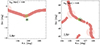 |
Fig. 1. Environment of two clusters: CL1052 (left panel), which is one of the most distant clusters from filaments, and CL3030 (right panel), which is a high surface brightness cluster with a typical (median) distance. Our clusters are marked by the black cross in the centre, the dark green circle represents their virial radii r200, filaments are in coral, and intersections (not used in this work) are in rose. The closest filament point, used for measuring the distance, is surrounded by a green rhombus. |
Distance between each cluster used in this work and its closest filament.
In Fig. 2, we show the distance between our clusters and the closest filament as a function of the X-ray surface brightness. It can be seen that the plot has a sort of triangular shape, with high surface brightness clusters found closer to filaments than the low surface brightness ones. In fact, no gas-rich cluster is found at more than 3 Mpc from filaments. On the other hand, gas-intermediate and gas-poor clusters (black and blue points, respectively) can be found at greater distances from filaments. Gas-rich and gas-intermediate clusters often have distances smaller than half Mpc, whereas gas-poor clusters are rarely found at distance smaller than 2 Mpc.
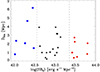 |
Fig. 2. Distance between our clusters and the nearest filament as a function of their X-ray surface brightness SBX. The figure is colour-coded according to the X-ray surface brightness: high surface brightness clusters are shown with red circles, low surface brightness with blue squares, and intermediate cases with black stars. The farthest object in our sample is highlighted with a blue open square, and it refers to CL1011, a peculiar case that we analyse in detail in Appendix A. |
There is also a sort of dichotomy in the cluster population of Fig. 2. In fact, there seems to be a diagonal gap covering all the surface brightness range. We model this possible dichotomy in Appendix B; however, we were unable to find any impact of this possible dichotomy on the global properties of clusters (halo mass, magnitude of the brightest cluster galaxies, magnitude gap, and X-ray temperature).
Finally, we plot in Fig. 3 the cumulative distribution of the distance from filaments for the three classes of objects. The two subsamples of gas-rich and gas-poor systems seem to follow different distributions. In particular, their median values are Dfila, rich = 0.98 Mpc and Dfila, rich = 2.20 Mpc. In Fig. 3, we also report the 25 and 75 percentile uncertainties. However, the Kolmogorov-Smirnov test, with a p-value of 0.35, is unable to reject the null hypothesis stating that the two samples are drawn from the same parent distribution. Using the model introduced in Appendix B, we found that the dependence of the distance from the filament on the cluster brightness is only about 1.5σ significant. Therefore, our evidence remains tentative only and requires a larger sample to be established with larger significance.
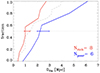 |
Fig. 3. Cumulative distribution of the distance to the nearest filament for clusters of large (red solid line), intermediate (black dashed line), and low surface brightness (blue solid line). The horizontal dotted line indicates the median of each distribution, and the limits of the error bars are the 25 and 75 percentile of each distribution. |
4. Discussion and conclusions
In this work we have computed the distance between a sample of clusters and the filaments of the cosmic web. We divided our sample into three subsamples according to their X-ray surface brightness, and we mainly focused our attention on the subsamples of high and low surface brightness clusters, with the third subsample being an intermediate case. As mentioned, X-ray surface brightness is tightly related to gas fraction (Andreon et al. 2017b; Ragagnin et al. 2022).
We found that there seems to be a trend in which, on average, gas-poor systems are found at greater distances than gas-rich ones. However the difference is statistically inconclusive, probably due to the small size of the sample since it has eight gas-rich clusters and six gas-poor ones.
The position of clusters within the cosmic web could have an impact on the mechanisms affecting their gas reservoir. The low gas fraction of some of our clusters (Andreon et al. 2017a) and the low values measured by Hadzhiyska et al. (2024) and Bigwood et al. (2024) all indicate that a considerable fraction (up to 50%) of the gas mass can be displaced away from the central regions. Indeed, Bigwood et al. (2024) observations constrained the lack to even larger radii, and Hadzhiyska et al. (2024) observations show that the gas is much more extended than the dark matter. Both studies interpret their results as being influenced by AGN feedback, which, according to Hadzhiyska et al. (2024), is stronger than that observed in the Illustris-TNG cosmological simulation (Nelson et al. 2019) and, as noted by Bigwood et al. (2024), stronger than in most modern simulations. The scatter in the gas fraction and its possible dependence on the cluster position in the cosmic web allow us to speculate that the presence of a filament may in part control the gas flow, as the gas driven at large radii by the AGN could find a stronger resistance from the filament, thus reducing the speed and the distance that can be reached by the gas displaced by the AGN feedback. Furthermore, since the gas is closer to the cluster centre than when there is an absence of a filament, the return would be faster once the AGN feedback is completed. Both effects would make clusters near the spine of filaments more gas rich and clusters further away more gas poor, as our observations seem to suggest. The identification of the mechanisms able to modulate the gas flow from and to large distances, such as the ones proposed above, is crucial for understanding the variety of gas fractions in both the central and non-central regions of galaxy clusters.
Concluding, in this work, we have studied a sample of 29 velocity dispersion-selected clusters classified in X-ray surface brightness classes, which are also gas-fraction classes, with the goal of analysing the large-scale structure around these objects and, in particular, their distance from the nearest filament. We find hints that gas-poor clusters are found, on average, at greater distances from filaments than gas-rich ones, although the small sample size prevents us from drawing definitive conclusions. A larger sample will certainly reduce the statistical uncertainty that is affecting our determination.
Acknowledgments
The authors thanks the referee for his/her prompt response and for his/her comments, which helped to improve the clarity and presentation of our results. SZ acknowledges the financial support provided by the Governments of Spain and Aragón through their general budgets and the Fondo de Inversiones de Teruel, the Aragonese Government through the Research Group E16_23R, the Spanish Ministry of Science and Innovation (MCIN/AEI/10.13039/501100011033) and ERDF, A way of making Europe with grant PID2021-124918NB-C44, and from the Spanish Ministry of Science and Innovation and the European Union – NextGenerationEU through the Recovery and Resilience Facility project ICTS-MRR-2021-03-CEFCA. SA and EP acknowledge PRIN-MIUR grant 20228B938N “Mass and selection biases of galaxy clusters: a multi-probe approach”. SA acknowledges INAF grant “Characterizing the newly discovered clusters of low surface brightness”.
References
- Abazajian, K., Adelman-McCarthy, J. K., Agüeros, M. A., et al. 2004, AJ, 128, 502 [NASA ADS] [CrossRef] [Google Scholar]
- Alam, S., Albareti, F. D., Allende Prieto, C., et al. 2015, ApJS, 219, 12 [Google Scholar]
- Andreon, S., & Hurn, M. A. 2010, MNRAS, 404, 1922 [NASA ADS] [Google Scholar]
- Andreon, S., & Moretti, A. 2011, A&A, 536, A37 [NASA ADS] [CrossRef] [EDP Sciences] [Google Scholar]
- Andreon, S., Trinchieri, G., & Pizzolato, F. 2011, MNRAS, 412, 2391 [NASA ADS] [CrossRef] [Google Scholar]
- Andreon, S., Serra, A. L., Moretti, A., & Trinchieri, G. 2016, A&A, 585, A147 [NASA ADS] [CrossRef] [EDP Sciences] [Google Scholar]
- Andreon, S., Wang, J., Trinchieri, G., Moretti, A., & Serra, A. L. 2017a, A&A, 606, A24 [NASA ADS] [CrossRef] [EDP Sciences] [Google Scholar]
- Andreon, S., Trinchieri, G., Moretti, A., & Wang, J. 2017b, A&A, 606, A25 [NASA ADS] [CrossRef] [EDP Sciences] [Google Scholar]
- Andreon, S., Trinchieri, G., & Moretti, A. 2022, MNRAS, 511, 4991 [NASA ADS] [CrossRef] [Google Scholar]
- Andreon, S., Trinchieri, G., & Moretti, A. 2024, A&A, 686, A284 [NASA ADS] [CrossRef] [EDP Sciences] [Google Scholar]
- Bigwood, L., Amon, A., Schneider, A., et al. 2024, MNRAS, 534, 655 [NASA ADS] [CrossRef] [Google Scholar]
- Brunner, H., Liu, T., Lamer, G., et al. 2022, A&A, 661, A1 [NASA ADS] [CrossRef] [EDP Sciences] [Google Scholar]
- Chen, Y.-C., Ho, S., Brinkmann, J., et al. 2016, MNRAS, 461, 3896 [NASA ADS] [CrossRef] [Google Scholar]
- Diaferio, A. 1999, MNRAS, 309, 610 [CrossRef] [Google Scholar]
- Diaferio, A., & Geller, M. J. 1997, ApJ, 481, 633 [NASA ADS] [CrossRef] [Google Scholar]
- Driver, S. P., Bellstedt, S., Robotham, A. S. G., et al. 2022, MNRAS, 513, 439 [NASA ADS] [CrossRef] [Google Scholar]
- Eckert, D., Molendi, S., & Paltani, S. 2011, A&A, 526, A79 [NASA ADS] [CrossRef] [EDP Sciences] [Google Scholar]
- Gouin, C., Gallo, S., & Aghanim, N. 2022, A&A, 664, A198 [NASA ADS] [CrossRef] [EDP Sciences] [Google Scholar]
- Hadzhiyska, B., Ferraro, S., Ried Guachalla, B., et al. 2024, arXiv e-prints [arXiv:2407.07152] [Google Scholar]
- Miller, C. J., Nichol, R. C., Reichart, D., et al. 2005, AJ, 130, 968 [Google Scholar]
- Nelson, D., Springel, V., Pillepich, A., et al. 2019, Comput. Astrophys. Cosmol., 6, 2 [Google Scholar]
- Pacaud, F., Pierre, M., Adami, C., et al. 2007, MNRAS, 382, 1289 [Google Scholar]
- Planck Collaboration IX. 2011, A&A, 536, A9 [NASA ADS] [CrossRef] [EDP Sciences] [Google Scholar]
- Plummer, M. 2010, JAGS Version 2.2.0331 user manual [Google Scholar]
- Popesso, P., Biviano, A., Bulbul, E., et al. 2024, MNRAS, 527, 895 [Google Scholar]
- Puddu, E., & Andreon, S. 2022, MNRAS, 511, 2968 [NASA ADS] [CrossRef] [Google Scholar]
- Ragagnin, A., Andreon, S., & Puddu, E. 2022, A&A, 666, A22 [NASA ADS] [CrossRef] [EDP Sciences] [Google Scholar]
- Santoni, S., De Petris, M., Ferragamo, A., Yepes, G., & Cui, W. 2024, in mm Universe 2023 - Observing the Universe at mm Wavelengths, European Physical Journal Web of Conferences, 293, 00048 [NASA ADS] [Google Scholar]
- Serra, A. L., Diaferio, A., Murante, G., & Borgani, S. 2011, MNRAS, 412, 800 [NASA ADS] [Google Scholar]
- Stanek, R., Evrard, A. E., Böhringer, H., Schuecker, P., & Nord, B. 2006, ApJ, 648, 956 [NASA ADS] [CrossRef] [Google Scholar]
- Sunyaev, R. A., & Zeldovich, Y. B. 1972, Comm. Astrophys. Space Phys., 4, 173 [Google Scholar]
- Zarattini, S., Aguerri, J. A. L., Calvi, R., & Girardi, M. 2022, A&A, 668, A38 [NASA ADS] [CrossRef] [EDP Sciences] [Google Scholar]
- Zarattini, S., Aguerri, J. A. L., TarrÃo, P., & Corsini, E. M. 2023, A&A, 676, A133 [NASA ADS] [CrossRef] [EDP Sciences] [Google Scholar]
Appendix A: Caveats on the filament catalogue: The case of CL1011
As mentioned in Sect. 2, the catalogue from Chen et al. (2016) is based on the SDSS DR12 data. These data are homogeneous on a large-scale basis but can suffer for incompleteness due to various caveats (e.g. fibre collisions, presence of bright stars that exclude areas from the spectroscopic follow up) that can lead to an incomplete detection of filaments. For the cluster CL1011, that is the gas-poor cluster with the greatest distance to filaments in our sample, we notice a truncated filament that could become the nearest one, if extended towards the cluster. A possible explanation is that the filament is aligned along the line of sight. In this case, due to the construction of the filament catalogue, we expect the missing part of the filament to be found in one of the contiguous redshift slices. In Fig. A.1 we show the large-scale structure of CL1011, including the filaments in the previous and following redshift slices (in blue and red, respectively), to understand the tridimensional structure of this region. There are two filaments, one in the former and one in the latter slice, but no one is the extension of the truncated filament. Of course, the filament could be missing due to incompleteness in the SDSS spectroscopy or in a caveat in the detection code. However, given the lack of concrete evidence, we must rely on the Chen et al. (2016) catalogue, as we have done throughout the rest of our work.
It is worth noticing, however, that CL1011 is the only cluster in our sample for which we suspect a possible problem in the Chen et al. (2016) catalogue of filament, so we do not think that this issue is affecting the general result. However, it happens to coincide with the system at the greatest distance, the only one outside the triangular shape that we find in Fig. 2. In particular, the distance that we measured for the second most-distant cluster (Dfila = 4.6 Mpc) seems robust.
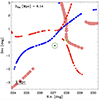 |
Fig. A.1. Large-scale structure around CL1011. The filaments and intersections in the correct redshift slice are reported in light coral and rose, as in Fig. 1. The green rhombus is the point to which the distance was measured. We also plot the filaments of the preceding (0.085 ≤ z < 0.09, in blue) and succeeding (0.095 ≤ z < 0.10, in red) redshift slices in order to look for filaments along the line of sight (e.g. extensions of filaments across different slices). None were found. |
Appendix B: Modelling of the distance from the filament versus X-ray brightness distribution
We notice that there is a possible dichotomy in the distribution of points of Fig. 2. In fact, there is a sort of diagonal gap in that figure. We therefore fit the whole data with a mixture of two linear regressions with a Student-t scatter (with 10 degrees of freedom) around them. The latter is taken because it is robust to outliers (Andreon & Hurn 2010). We took uniform priors for the probability of belonging to the population with small distance, for the scatters, the intercepts, and the angles (i.e. a Student-t distribution with 1 degree of freedom on the slopes, Andreon & Hurn 2010). We fit all the data, without assuming which points are drawn from which population, and we sample the posterior with a Gibb sampler (JAGS, Plummer 2010). For parameter identifiability, the second population is the one with a greater distance (i.e. with larger intercept, evaluated at 43.0 erg s−1 Mpc−2). Fig. B.1 illustrates that most points quite neatly split in two nearly separated populations (p is ∼0 or ∼1; i.e. yellow or blue) and that the two relations have clearly different intercepts. In other terms, the data can be successfully divided in two unmixed populations. However, we did not find any particular relation characterising the two subsamples in terms of halo mass, the magnitude of the BCG, the magnitude difference between the two brightest members, and the X-ray temperature. Therefore, we conclude that the observed dichotomy, though successfully modelled, either results from the small sample size or is real but has no impact on the features discussed above. The model in which both slopes are set to zero—meaning that the distance from the filament is independent of the cluster brightness—can only be rejected at approximately 1.5σ.
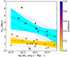 |
Fig. B.1. Distance between our clusters and the nearest filament as a function of their X-ray surface brightness SBX. Points are colour-coded according to probability of belonging to the more distant population. Shading indicates the 68% error on the fit, whereas the dashed corridors indicate ±1 the estimated scatter around the mean relation. |
All Tables
All Figures
|
Fig. 1. Environment of two clusters: CL1052 (left panel), which is one of the most distant clusters from filaments, and CL3030 (right panel), which is a high surface brightness cluster with a typical (median) distance. Our clusters are marked by the black cross in the centre, the dark green circle represents their virial radii r200, filaments are in coral, and intersections (not used in this work) are in rose. The closest filament point, used for measuring the distance, is surrounded by a green rhombus. |
| In the text | |
|
Fig. 2. Distance between our clusters and the nearest filament as a function of their X-ray surface brightness SBX. The figure is colour-coded according to the X-ray surface brightness: high surface brightness clusters are shown with red circles, low surface brightness with blue squares, and intermediate cases with black stars. The farthest object in our sample is highlighted with a blue open square, and it refers to CL1011, a peculiar case that we analyse in detail in Appendix A. |
| In the text | |
|
Fig. 3. Cumulative distribution of the distance to the nearest filament for clusters of large (red solid line), intermediate (black dashed line), and low surface brightness (blue solid line). The horizontal dotted line indicates the median of each distribution, and the limits of the error bars are the 25 and 75 percentile of each distribution. |
| In the text | |
|
Fig. A.1. Large-scale structure around CL1011. The filaments and intersections in the correct redshift slice are reported in light coral and rose, as in Fig. 1. The green rhombus is the point to which the distance was measured. We also plot the filaments of the preceding (0.085 ≤ z < 0.09, in blue) and succeeding (0.095 ≤ z < 0.10, in red) redshift slices in order to look for filaments along the line of sight (e.g. extensions of filaments across different slices). None were found. |
| In the text | |
|
Fig. B.1. Distance between our clusters and the nearest filament as a function of their X-ray surface brightness SBX. Points are colour-coded according to probability of belonging to the more distant population. Shading indicates the 68% error on the fit, whereas the dashed corridors indicate ±1 the estimated scatter around the mean relation. |
| In the text | |
Current usage metrics show cumulative count of Article Views (full-text article views including HTML views, PDF and ePub downloads, according to the available data) and Abstracts Views on Vision4Press platform.
Data correspond to usage on the plateform after 2015. The current usage metrics is available 48-96 hours after online publication and is updated daily on week days.
Initial download of the metrics may take a while.