| Issue |
A&A
Volume 694, February 2025
|
|
|---|---|---|
| Article Number | A268 | |
| Number of page(s) | 19 | |
| Section | Planets, planetary systems, and small bodies | |
| DOI | https://doi.org/10.1051/0004-6361/202452517 | |
| Published online | 19 February 2025 | |
Three warm Jupiters orbiting TOI-6628, TOI-3837, and TOI-5027 and one sub-Saturn orbiting TOI-2328★
1
Facultad de Ingeniería y Ciencias, Universidad Adolfo Ibáñez,
Av. Diagonal las Torres 2640,
Peñalolén, Santiago,
Chile
2
Millennium Institute for Astrophysics,
Santiago,
Chile
3
Data Observatory Foundation,
Santiago,
Chile
4
El Sauce Observatory – Obstech,
Coquimbo,
Chile
5
Max-Planck-Institut für Astronomie,
Königstuhl 17,
69117
Heidelberg,
Germany
6
European Southern Observatory (ESO),
Avenida Alonso de Córdova 3107,
Vitacura, Santiago,
Chile
7
Space Telescope Science Institute,
3700 San Martin Drive,
Baltimore,
MD
21218,
USA
8
Observatoire de Genève, Département d’Astronomie, Université de Genève,
Chemin Pegasi 51b,
1290
Versoix,
Switzerland
9
Instituto de Astrofísica, Facultad de Física, Pontificia Universidad Católica de Chile,
Av. Vicuña Mackenna 4860,
Santiago,
Chile
10
Department of Astronomy/Steward Observatory, The University of Arizona,
933 North Cherry Avenue,
Tucson,
AZ
85721,
USA
11
Landessternwarte, Zentrum für Astronomie der Universtät Heidelberg,
Königstuhl 12,
69117
Heidelberg,
Germany
12
Department of Astronomy, Sofia University St Kliment Ohridski,
5 James Bourchier Blvd,
1164
Sofia,
Bulgaria
13
Department of Astrophysical Sciences, Princeton University,
Princeton,
NJ
08544,
USA
14
Cavendish Laboratory,
J.J. Thomson Avenue,
Cambridge
CB3 0HE,
UK
15
Department of Physics, Cornell University,
Ithaca,
NY,
USA
16
Carnegie Institution for Science, Earth & Planets Laboratory,
5241 Broad Branch Road NW,
Washington,
DC
20015,
U.S.A.
17
The Observatories of the Carnegie Institution for Science,
813 Santa Barbara Street,
Pasadena,
CA
91101,
USA
18
Las Campanas Observatory, Carnegie Institution of Washington, Colina el Pino,
Casilla 601
La Serena,
Chile
19
Department of Physics and Kavli Institute for Astrophysics and Space Research, Massachusetts Institute of Technology,
77 Massachusetts Avenue,
Cambridge,
MA
02139,
USA
20
Center for Astrophysics | Harvard & Smithsonian,
60 Garden Street,
Cambridge,
MA
02138,
USA
21
Hazelwood Observatory,
RMB 4036 Matta Drive, Hazelwood South,
Victoria
3840,
Australia
22
Department of Physics & Astronomy, Johns Hopkins University,
3400 N. Charles Street,
Baltimore,
MD
21218,
USA
23
Società Astronomica Lunae,
Castelnuovo Magra,
Italy
24
Department of Earth, Atmospheric and Planetary Sciences, Massachusetts Institute of Technology,
77 Massachusetts Avenue,
Cambridge,
MA
02139,
USA
25
Department of Aeronautics and Astronautics, Massachusetts Institute of Technology,
77 Massachusetts Avenue,
Cambridge,
MA
02139,
USA
26
NASA Ames Research Center,
Moffett Field,
CA
94035,
USA
27
Department of Astronomy, Yale University,
219 Prospect Street,
New Haven,
CT 06511,
USA
28
Department of Physics and Astronomy, The University of New Mexico,
210 Yale Blvd NE,
Albuquerque,
NM
87106,
USA
★★ Corresponding author; This email address is being protected from spambots. You need JavaScript enabled to view it.
Received:
7
October
2024
Accepted:
3
January
2025
Abstract
We report the discovery and characterization of three new transiting giant planets orbiting TOI-6628, TOI-3837, and TOI-5027 and one new warm sub-Saturn orbiting TOI-2328, whose transits events were detected in the light curves of the Transiting Exoplanet Survey Satellite (TESS) space mission. By combining TESS light curves with ground-based photometric and spectroscopic followup observations, we confirm the planetary nature of the observed transits and radial velocity variations. TOI-6628 b has a mass of 0.74±0.06 MJ and a radius of 0.98−0.05+0.06 RJ and orbits a metal-rich star with a period of 18.18424 ± 0.00001 days and an eccentricity of 0.670−0.016+0.015, making it one of the most eccentric orbits of all known warm giants. TOI-3837 b has a mass of 0.59±0.05 MJ and a radius of 0.97−0.06+0.05 RJ and orbits its host star every 11.88865 ± 0.00003 days, with a moderate eccentricity of 0.221−0.046+0.042. With a mass of 2.02±0.13 MJ and a radius of 0.96−0.06+0.05 RJ, TOI-5027 b orbits its host star in an eccentric orbit with e = 0.385−0.026+0.025 every 10.24368±0.00001 days. TOI-2328 b is a Saturn-like planet with a mass of 0.16±0.02 MJ and a radius of 0.89−0.05+0.04 RJ; it orbits its host star in a nearly circular orbit with e = 0.057−0.029+0.046 at a period of 17.10197±0.00001 days. All four planets have orbital periods above ten days, and our planet’s interior structure models are consistent with a rocky-icy core with an H/He envelope, providing evidence supporting the core-accretion model of planet formation for this kind of planet.
Key words: techniques: radial velocities / planets and satellites: detection / planets and satellites: gaseous planets / planets and satellites: interiors
Based on observations collected at La Silla Observatory under program IDs 0103.A-9008(A), 0104.A-9007(A), 0104.C-0413(A), 0105.A- 9001(A), 0106.A-9014(A), 0109.A-9003(A), 0110.A-9011(A), 0111.A-9011(A), 105.20GX.001, 106.21ER.001, 108.22A8.001, and 109.239V.001, and through the Chilean Telescope Time under programs CN2020B-21, CN2021A-14, and CN2021B-23. This paper includes data gathered with the 6.5 meter Magellan Telescopes located at Las Campanas Observatory, Chile.
© The Authors 2025
 Open Access article, published by EDP Sciences, under the terms of the Creative Commons Attribution License (https://creativecommons.org/licenses/by/4.0), which permits unrestricted use, distribution, and reproduction in any medium, provided the original work is properly cited.
This article is published in open access under the Subscribe to Open model. This email address is being protected from spambots. You need JavaScript enabled to view it. to support open access publication.
1 Introduction
The increasing number and diversity of exoplanets discovered in recent decades has raised fundamental questions about their formation and evolution mechanisms. Many of these planets are giant planets orbiting very close to their host star, despite the low occurrence rate of this population (Stevenson 1982; Mayor et al. 2011; Fressin et al. 2013; Santerne et al. 2016). This is mainly driven by the inherent observational bias in their detection, given their small periods, which results in a dominant population of hot Jupiters (HJs) – highly irradiated planets given their proximity to their host star – which constitute about 75% of the well- characterized transiting planets – planets with radii and masses measured with an uncertainty better than about 20%. Most of such discoveries were made by wide-field ground-based observatories (Bakos et al. 2006; Mandushev et al. 2005; Udalski et al. 2002) by the Kepler and K2 space missions (Borucki 2017; Howell et al. 2014) and more recently by the Transiting Exoplanet Survey Satellite mission (TESS; Ricker et al. 2015).
Giant planets are believed to form via two different mechanisms: either by accreting its mass from the proto-planetary disk (Pollack et al. 1996) or by gravitational instabilities in which the proto-planetary disk fragments into bound clumps to form a planet (Cameron 1978). Both mechanisms predict a low formation rate at close-in orbits. Close to the star, gas conditions could prevent the formation of bound clumps (Rafikov 2005), while at the same time such conditions may prevent the formation of cores large enough to accrete gas from the proto-planetary disk (Schlichting 2014). Therefore, the observed population of HJs strongly suggests that they might have formed further out – in regions where the conditions for core accretion and gravitational instabilities are more favorable – and migrated inwards into their currently close-in circular orbits.
Possible migration mechanisms consider interactions with the disk (e.g. Walsh et al. 2011) and tidal migration produced by changes in the orbit, which can be induced by planet–planet scattering (Rasio & Ford 1996) or cyclic and/or chaotic secular interactions (Kozai 1962; Lidov 1962; Wu & Lithwick 2011). Both mechanisms predict different orbital parameters for planet populations. Although disk migration mainly predicts circular orbits aligned with stellar spin, high-eccentricity migration predicts a wide distribution of eccentricities and obliquities (Chatterjee et al. 2008). In this context, estimation of the bulk structures and atmospheric parameters of such populations of exoplanets could provide crucial information about their formation locations in the disk and possible migration paths (Madhusudhan et al. 2014; Mollière et al. 2022).
The characterization of the HJ formation history, widely defined as planets with masses greater than about 0.25 MJ and periods shorter than ten days (Dawson & Johnson 2018), may be problematic, as their proximity to their host star may induce radiative and tidal interactions that can affect the interpretation of the origins of the observed population (e.g., Albrecht et al. 2012). Therefore, giant planets – widely defined as planets with masses between about 0.3 MJ and 60 MJ (Hatzes & Rauer 2015) – within the snow line but farther from their host star, represent a unique opportunity to study possible formation and migration mechanisms in giant planets, as they are significantly less affected by their proximity to their host star. This allows a more direct comparison of their orbital properties with formation and migration models.
Warm Jupiters (WJs), generally defined as planets larger than six Earth radii, with masses larger than 1/3 of Jupiter’s mass, and with orbital periods between eight and 200 days (Dong et al. 2021), remained elusive for ground-based transit searches, mainly due to the constraints imposed by the daily cycle. Although some detections were possible with the Kepler (8 WJs1) and K2 (37 WJs1) missions (i.e., Huang et al. 2016), only with TESS has it been possible to systematically characterize them thanks to its significantly larger field of view, either through the detection of periodic transit signals or single transiters (e.g., Brahm et al. 2019 and Gill et al. 2020). It is expected that TESS will significantly increase the number of WJ detections (Barclay et al. 2018), despite its limitations in detecting longer period planets given its observing strategy; that is, TESS observes each sector of the sky for approximately 30 days and observes much brighter stars, giving us the opportunity to confirm the planetary signals with spectroscopic observations. By complementing transit observations with radial velocity (RV) measurements, it is possible to provide a detailed characterization of the dynamical and physical properties of the planetary system.
The Warm gIaNts with TESS (WINE) collaboration is a dedicated survey to identify, confirm, and characterize WJs using TESS data and ground-based photometric and spectroscopic follow-up facilities, with the main goal of building a WJ database to constrain theories of planetary formation and evolution (Kossakowski et al. 2019; Jordán et al. 2020; Brahm et al. 2020, 2023; Schlecker et al. 2020; Hobson et al. 2021, 2023; Trifonov et al. 2021, 2023; Jones et al. 2024). Here, we present the discovery, confirmation, and orbital characterization of four new transiting exoplanets by the WINE collaboration; three of them are WJs, and one is a Saturn-like planet, the latter labeled as such because of its low mass.
The paper is organized as follows. In Sect. 2, we present our observations. In Sect. 3, we present stellar parameters of the stars under study. In Sect. 4, we provide the orbital parameters of the planetary systems, and in Sect. 5 we give the modeling of the planetary interiors. We provide a discussion of our results in Sect. 6, and in Sect. 7 we present our conclusions.
2 Observations
2.1 TESS
All four transiting candidates presented in this study were identified from the full-frame image (FFI) light curves of the TESS primary mission. The FFIs were calibrated by the Science Processing Operations Center (SPOC) at NASA Ames Research Center (Jenkins et al. 2016). Table 1 summarizes the details of the TESS observations.
The TOIs 6628.01, 3837.01, and 5027.01 were also detected by the FAINT search pipeline (Kunimoto & Daylan 2021) and reported to the community by the TESS Science Office on 15 August, 2023, 23 June, 2021, and 6 January, 2022 after review by the TESS Science Office (Guerrero et al. 2021). TOI-2328.01 was also detected by the SPOC transit search pipeline and communicated to the community on 7 October, 2020. The difference-image-centroiding analysis (Twicken et al. 2018) presented in the SPOC Data Validation reports for TOIs 3837, 5027, and 2328 constrained the location of the source of the transit signatures to within 0.219±2.4 arcsec (Sector 45), 0.951±2.5 arcsec (Sector 66), and 0.330±2.5 arcsec (Sectors 1– 68), respectively. We chose the sectors that provided the best results in the analysis of the target centroid. We did not find any SPOC Data Validation report for TOI-6628.
Due to our focus on the detection of transiting giant planets in long-period orbits (P>10 days), we process all the light curves with a dedicated algorithm that, after passing them through a median filter, identifies systematic negative deviations in flux, whose amplitudes could be consistent with the depths and durations of transits of giant planets orbiting main-sequence/subgiant stars. All systems that present such specific variations are then manually vetted. The possible dilution of the transits by neighboring stars that fall inside the TESS photometric aperture is considered in the manual vetting process when estimating the planet radius from the transit depth and host stellar radius.
We also obtained two-minute cadence light curves from the Mikulski Archive for Space Telescopes (MAST). We used data calculated by SPOC, which provides simple aperture photometry (SAP) and systematics-corrected Presearch Data Conditioning photometry (PDC; Smith et al. 2012; Stumpe et al. 2012; Stumpe et al. 2014). We also used data calculated by the Quick Look Pipeline (QLP, Huang et al. 2020a,b; Kunimoto et al. 2021, 2022).
To study possible contamination from other sources, we analyzed the target pixel files (TPFs). Figure 1 shows the TPFs for the sectors in which the first transit was detected for the four targets under study. The TPF plots show the field around the observed target and the aperture mask used in the light-curve construction. The PDC-SAP data from MAST have already been corrected by the contamination of neighboring stars and instrumental systematics (Stumpe et al. 2012); therefore, no dilution correction is applied to these light curves in the joint-fit analysis of the transit and RV data. We only studied the possible effects of dilution in the analysis of false-positive scenarios of TOI-3837.01 transits presented in Sect. 4.1.2, because there is an object located at an angular separation of about 0.4 arcsec.
All four targets were selected as high-priority candidates for the WINE collaboration and are suitable for spectroscopic follow-up. TOI-6628 was observed by TESS in sectors 11, 38, and 65. We identified five transit events with an average depth of 7500 ppm and a duration of ∼0.2 days in the TESS light curves. A query to the Gaia DR3 archive (Gaia Collaboration 2016, 2023) revealed five neighboring stars within a 15″ radius with Gaia magnitudes larger than 18. The difference in magnitude between TOI-6628 and these targets is more than five; therefore, their contamination of the flux measured in the light curve is less than 1% in all cases. This flux difference corresponds to a planetary radius of less than about 0.01, a value smaller than the uncertainty of the derived planet radius. Therefore, we neglect the effect of these nearby objects in the data analysis. The brightest star close to TOI-6628 has a magnitude of 12.91. In addition, we observe three other stars in the nearby field with magnitudes of about 14 mag. Such targets can be observed in the TESS TPF, shown in Fig. 1, together with the aperture mask employed by the TESS pipeline, which is shown by red striped squares. Given the proximity of the 14.13 mag star to our target – their angular separation is about 40 arcsec – we may expect some minor contamination on the order of 25% in flux from this target in one of the pixels of the aperture mask, which amounts to a possible contamination of 3.5% in the light curve considering that it is built using the seven pixels of the aperture mask. This contribution is smaller than the uncertainty of the planet radius derived; therefore, we neglect their effect in our data analysis. We acknowledge that TOI-6628 was also observed from ground-based telescopes with a much larger pixel scale, avoiding contamination from nearby objects and confirming the transiting signal in TOI-6628.01.
TOI-3837 was observed by TESS in sector 21 and then revisited in sectors 45, 46, and 48. We identified seven transits in the TESS light curves, with an average depth of about 7000 ppm and a transit duration of 0.22 days. A query to the Gaia DR3 archive reveals that there are no stars within a 30″ radius, which is in agreement with the TESS TPF image shown in Fig. 1.
TOI-5027 was observed by TESS in sectors 12, 39, and 66. Six transit events with an average depth of about 10800 ppm and a duration of ∼0.14 days were identified in the TESS light curves. A query to the Gaia DR3 archive revealed six neighboring stars closer than 30″. All such neighboring targets have magnitudes over 18. Their flux contamination is less than 1%; therefore, we neglected the effect of these nearby objects in the TOI-5027 light curves. We observe an object at an angular distance of 23 arcsec with a magnitude of 14.8. We expect a contamination of about 3% in one of the top pixels of the aperture mask from this target, which amounts to a possible contamination of less than 1% of the light curve considering that it is built using the eight pixels of the aperture mask. This contribution is smaller than the uncertainty of the planet radius derived; therefore, we neglected their effect in our data analysis. Moreover, we do observe a nearby bright companion with a Gaia magnitude of 10.61, but it is located outside the TESS aperture masks. TOI-5027 was also observed from ground-based telescopes with a much smaller pixel scale, avoiding contamination from nearby objects and confirming the transit signal in TOI-5027.01.
TOI-2328 was observed by TESS in sectors 1, 13, 27, 28, 39, 67, and 68. We identified ten transits in the TESS light curves, with a transit depth of about 10400 ppm and a transit duration of about 0.15 days. A query to the Gaia DR3 data archive reveals a neighbor star with a magnitude of about 17 within a 15″ radius, which contributes a flux contamination under 1%. An additional bright target with a Gaia magnitude of 12.62 is located about 3 arcmin from our target, but it does not contaminate the aperture mask. This target can be observed in the sector 13 TPF image shown in Fig. 1.
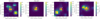 |
Fig. 1 TESS target pixel files (TPF) of TOI-6628, TOI-3837, TOI-5027, and TOI-2328. We show the aperture mask used in the light-curve measurement with red striped squares. We indicate the Gaia (Gaia Collaboration 2018) magnitudes of the targets and surrounding stars. |
TESS observations of the targets presented here.
Ground-based follow-up observations obtained for the targets presented here.
2.2 Ground-based photometry
We used ground-based photometric time series obtained with submeter-class telescopes to confirm the planetary nature of transiting candidates identified by TESS. These light curves are used to ensure that the transit-like feature occurs on the particular star of interest, and not on another star inside the photometric aperture of the TESS data. Given the low number of transits present in the TESS data for the four systems presented in this study, these additional light curves are also crucial for refining the photometric ephemeris. Table 2 shows the details of the ground-based follow-up observations of the planetary systems under study, and Fig. 2 shows the ground-based light curves along with the phase-folded TESS light curves.
2.2.1 Observatoire Moana
Observatoire Moana is a global network of telescopes with observation stations in Chile, Europe, and Australia. The observations cited here were made by OMES–CDK600 and OMES–RiDK500, both of which are located at El Sauce Observatory, Chile. OMES–CDK600 is an equatorial fork-mounted, 0.6 meter diameter, corrected Dall-Kirkham telescope; and OMES–RiDK500 is a similarly mounted 0.5 meter Riccardi Dall-Kirkham instrument. Both telescopes are equipped with a range of filters, including the Sloan r filter and Andor Ikon-L 936 cameras with deep-depleted back-illuminated 2K×2K CCD sensors. OMES–CDK600 has a pixel scale of 0.67″ and a field of view of 0.4×0.4 degrees, and OMES–RiDK500 has a pixel scale of 0.78″ and a field of view of 0.6×0.6 degrees.
Reduction was performed using a dedicated automated pipeline that considers all sources available in the field and produces light curves and artificial comparison stars for all qualifying sources (derived from parameterized limits on variability and magnitude differentials) and an optimization algorithm that also draws on the spatial separation between targets and other sources. We observed two full transits of TOI-6628 b on the nights of 19 June, 2021 using OMES-CDK600 and one transit during the night of 15 March, 2024 using OMES-RiDK500.
We observed an almost-full transit of TOI-5027 b using OMES-RiDK500 on the night of 21 March, 2024. We observed half a transit of TOI-2328 b, including the planetary egress, on the night of 23 October, 2021 using OMES-CDK600.
2.2.2 CHAT
The Chilean Hungarian Automated Telescope (CHAT) was a robotic facility installed on Las Campanas Observatory in Chile.
CHAT consists of a FORNAX 200 equatorial mount and a 0.7-m telescope coupled with an FLI ML-23042 2048×2048 pixel CCD, which delivers a pixel scale of 0.6″/pixel. CHAT contains a set of i′ , r′ , and 𝑔′ pass-band filters.
We observed the transit of TOI-2328 b with CHAT on the night of 26 December, 2019 with the r′ filter adopting an exposure time of 20s. We obtained 112 images of TOI- 2328. CHAT data were processed with a dedicated pipeline that performs differential aperture photometry, where optimal comparison sources and the radius of the photometric aperture are automatically selected (e.g., Espinoza et al. 2019; Jones et al. 2019; Jordán et al. 2019).
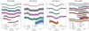 |
Fig. 2 Phase-folded light curve of TOI-6628.01, TOI-3837.01, TOI-5027.01, and TOI-2328.01. The best model is shown in black. |
2.2.3 LCOGT
Las Cumbres Observatory global telescope network (LCOGT; Brown et al. 2013) is a worldwide network of 1m telescopes, equipped with 4096×4096 SINISTRO cameras. The cameras have a pixel scale of 0.389 arcsec, resulting in a field of view of 26″×26″ , and they are equipped with SDSS/Pan-STARRS u′𝑔′r′i′zsYw filters. In addition, the LCOGT hosts a 0.35-m telescope equipped with a QHY600 detector and a i′ filter, providing a pixel scale of 0.75 arcsec.
We observed a full transit of TOI-6628 b on 26 May, 2024 with a cadence of five minutes using the LCOGT 0.35m telescope. We observed an almost-full transit of TOI-5027 b on 3 April, 2022 with a cadence of 2 min, and a full transit and an egress of TOI-2328 b on 24 September, 2020 and on 15 August, 2021, respectively, using the LCOGT 1m telescopes.
All transits were obtained using the i′ filter, except for the egress of TOI-2328 b, which was also observed using the g′ filter. All LCOGT science images were calibrated using the standard LCOGT BANZAI pipeline (McCully et al. 2018), and photometric measurements were extracted using AstroImageJ (Collins et al. 2017).
2.2.4 Hazelwood Observatory
The Hazelwood Observatory is a backyard observatory located in Victoria, Australia that has a 0.32m Planewave CDK F/8 telescope equipped with a SBIG STT3200 2.2k×1.5k CCD, providing a 20′×13′ field of view and plate scale of 0.55″ per pixel.
The system is equipped with a filter wheel with filters B, V, Rc, Ic, 𝑔′ , r′ , i′ and z′. We observed an ingress of TOI-6628 b on the night of 20 April, 2024 and an egress of TOI-2328 b on the night of 8 February, 2021, using the Rc filter on both occasions.
2.2.5 KeplerCam
KeplerCam is a 4K×4K CCD camera installed on the 1.2m Telescope at the Fred Lawrence Whipple Observatory (FLWO) in Mount Hopkins, Arizona, USA. The system provides a pixel scale of 0.672″ per pixel at 2×2 pixel binning. We obtained an egress of TOI-3837 b the night of 27 April, 2022 with a cadence of 30 seconds using the Sloan i′ filter.
2.3 Spectroscopy
We obtained precision radial velocities (RVs) for our four targets from three different instruments. The main goal is to search for RV variations that are consistent with the planetary hypotheses of the transiting planets. All FEROS and HARPS data obtained for this study were processed with the ceres pipeline (Brahm et al. 2017). ceres performs all the reduction steps to generate a continuum-normalized, wavelength-calibrated, and optimally extracted spectrum from raw data. ceres also computes precision radial velocities and bisector (BIS) spans through the cross-correlation technique. The BIS analysis of the crosscorrelation function (CCF) profile can be used as an indicator of phospheric activity (e.g., Queloz et al. 2001). We used a G2-type binary mask as a template to calculate the CCF of the spectra of our four candidates. All spectroscopic observations were obtained considering a telescope-pointing restriction of an angular distance of more than 30 degrees from the Moon to avoid light pollution. Table 3 shows the details of the RV observations.
2.3.1 FEROS
We used the Fiber-fed Extended Range Optical Spectrograph (FEROS; Kaufer et al. 1999) installed in the ESO-MPG 2.2 m telescope at La Silla Observatory, Chile, for spectroscopic follow-up. With an average resolving power of R ∼ 48 000, it can measure stellar RVs with an accuracy level on the order of a few meters per second, which is suitable for exoplanet searches.
The instrument is equipped with two fibers, allowing us to simultaneously observe the spectra of a secondary source for two purposes: to subtract the sky background or for simultaneous wavelength calibration. In our case, the latter was the observing mode chosen for our observations to optimize the RV precision of the measurements.
We obtained three RVs for TOI-6628 between 23 February, 2021 and 22 July, 2021, with a mean uncertainty of 9.3 m/s in the RVs. The observations were made with an exposure time of 25 min, resulting in an average signal-to-noise (S /N) = 53. Table A.1 shows the RVs obtained for TOI-6628.
We obtained eight RVs for TOI-3837 between 5 January, 2021 and 8 March, 2021. The mean uncertainty of the RVs is 10.1 m/s, with an exposure time of 15 min. The average S/N of the observations is 70. Table A.2 shows the RVs obtained for TOI-3837.
We obtained 27 RVs for TOI-5027 between 13 April, 2022 and 30 July, 2023. The mean uncertainty of the RVs is 11.2 m/s, which was obtained with an exposure time of 20 min. The average S/N of the observations is 80. Table A.3 shows the RVs obtained for TOI-5027.
We obtained 22 RVs for TOI-2328 between 11 July, 2022 and 23 November, 2022, with a mean RV uncertainty of 9.2 m/s. The observations were obtained with an exposure time of 20 min, reaching an average S/N of 50. Table A.4 shows the RVs obtained for TOI-2328.
RV observations obtained for the targets presented here.
2.3.2 HARPS
The High Accuracy Radial velocity Planet Searcher (HARPS; Mayor et al. 2003) is a fiber-fed, high-resolution, and stabilized spectrograph mounted on the Cassegrain focus of the ESO 3.6 m telescope of the ESO La Silla Observatory in Chile. It covers the spectral region of 380–690 nm, with a resolving power of R = 115 000, making it suitable for RV follow-up of exoplanets with a low semi-amplitude of RV variations.
We obtained 20 RVs for TOI-6628 between 18 March, 2021 and 11 September, 2022. The mean uncertainty of the RVs is 13.5 m/s, which was obtained with an exposure time of 30 min and an average S/N = 25. Table A.1 shows the RVs obtained for TOI-6628.
We obtained seven RVs for TOI-3837 between 4 February, 2021 and 21 March, 2021. The mean uncertainty of the RVs is 9.2 m/s, which was obtained in object-calibration mode with an exposure time of 20 min. The average S/N of the observations is 20. Table A.2 shows the RVs obtained for TOI-3837.
We obtained 22 RVs for TOI-2328 between 14 December, 2019 and 26 July, 2021. The mean uncertainty of the RVs is 8.3 m/s, which was obtained in object-calibration mode with an exposure time of 20 min and reached an average S/N = 25. Table A.4 shows the RVs obtained for TOI-2328.
2.3.3 PFS
We monitored TOI-2328 with the Planet Finder Spectrograph (PFS; Crane et al. 2006, 2008, 2010) installed at the 6.5-m Magellan/Clay telescope at Las Campanas Observatory. PFS can provide spectra with spectral resolving powers from 38 000 to 190 000. The target was observed using the instrument’s iodine gas-absorption cell during four different observation runs between 3 November, 2020 and 16 November, 2021, adopting an exposure time of 1200 s and using a 3×3 CCD binning mode to minimize readout noise. We also observed TOI-2328 without the iodine cell to generate a template to calculate the RVs, which were derived following the methodology of Butler et al. (1996). We obtained 12 RVs from PFS with a mean uncertainty of 5.7 m/s. The PFS RVs are presented in Table A.4.
2.4 High-resolution imaging
We used the optical speckle imaging technique to obtain high- resolution images for two of our targets: TOI-3837 and TOI- 5027. Both targets were observed with the HRCam of the Southern Astrophysical Research (SOAR) telescope (Tokovinin 2018; Ziegler et al. 2020), and TOI-3837 was also observed by the Sternberg Astronomical Institute (SAI) 2.5m telescope (Shatsky et al. 2020). The SOAR observations for TOI-3837 and TOI-5027 were obtained on 6 June, 2022 and on 22 April, 2022, respectively. The SAI-2.5 m telescope observation for TOI-3837 was obtained on 28 November, 2022.
No close companions were found for TOI-5027 at a contrast of ∆mag=6 at 1″. However, we identified a faint companion (∆I=4) of TOI-3837 at 0.4″ (see Fig. 3). The flux associated with the neighboring star might impact the determination of the physical parameters of the host star and the planetary transit parameters by diluting the transits. The flux contamination of this nearby target is approximately 2.5%. These effects are taken into account in the analysis of the TOI-3837 b system presented in Sect. 4.
3 Stellar parameters
Table 4 shows the main stellar parameters of our targets. The sky position’s right ascension (RA) and declination (Dec) are obtained from Gaia DR3 (Gaia Collaboration 2016, 2023), as are the proper motions and the stellar parallax π. We also show the TESS magnitude T (Ricker et al. 2015); the V and B magnitudes (Munari et al. 2014); the G magnitude (Gaia Collaboration 2018); and the J, H, and K magnitudes (Skrutskie et al. 2006). Using these data, we derived the stellar properties of the four host stars using the Zonal Atmospheric Stellar Parameters Estimator (zaspe, Brahm et al. 2017) code, following the iterative procedure described by Brahm et al. (2019).
First, we create a high S/N stellar template from the co-added stellar spectra, after removing the BERV and RV variations, which are observed for each star. This stellar template is then compared to a grid of synthetic spectra from the ATLAS9 models (Castelli & Kurucz 2003). After that, zaspe derives an initial set of stellar atmospheric parameters, namely effective temperature (Teff), surface gravity (log𝑔), metalicity ([Fe/H]), and projected rotational velocity (v sini). Then, the star’s physical parameters, mass (M*), radius (R*), luminosity (L*), density ρ*, stellar age, and visual extinction along the line of sight (AV) are obtained by comparing the stellar broad-band photometry with the synthetic magnitudes from the parsec stellar evolutionary models (Bressan et al. 2012). Absolute magnitudes are obtained using Gaia (Gaia Collaboration 2018) parallaxes.
We used the value Teff as prior to the calculation of the physical parameters with parsec. Although the value of [Fe/H] remains fixed2, Teff is used as an initial value in the calculation. The procedure is repeated in an iterative way until it converges.
Following Tayar et al. (2022), we add systematic uncertainties of 2% to the stellar luminosity, an uncertainty of 4% to the stellar radius, an uncertainty of 5% to the stellar mass, and an uncertainty of 20% to the stellar age. The resulting stellar parameters for the four stars here presented are listed in Table 4.
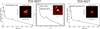 |
Fig. 3 High-resolution images of TOI-3837 and TOI-5027. |
Stellar parameters.
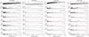 |
Fig. 4 Periodograms of photometric and spectroscopic data of TOI-6628, TOI-3837, TOI-5027, and TOI-2328, respectively. The horizontal red dashed line corresponds to the GLS 1% false alarm probability and the blue vertical dashed line marking the planet period. |
3.1 Activity indices
We computed stellar activity indices from the reduced data using ceres. Besides the bisectors of the CCF, we computed the Hα, NaII, HeI, and Call indices, which can be used as tracers of chromospheric activity (Andretta et al. 2005). For the Hα index, we followed the definition from Boisse et al. (2009). For the NaII and HeI indices, we followed the definition from Gomes da Silva et al. (2011). For the CaII index, we followed the definition from Duncan et al. (1991). In Table 4, we show the  values computed for the four stars from the co-added spectra, following the definition from Noyes et al. (1984)3. The activity indices for TOI-6628, TOI-3837, TOI-5027, and TOI-2328 are listed in Tables A.1, A.2, A.3, and A.4, and they are shown against the RVs in Figs. A.1, A.2, A.3, and A.4, respectively.
4 Analysis and results
We analyzed the transits and RV time series of the four systems to search for periodic signals. We computed the box least-square periodogram (BLS; Kovács et al. 2002) in the photometry time series by combining the data of the different instruments and epochs for each target. To search for periodicities in the RVs, and in the corresponding activity indices, we computed the generalized Lomb–Scargle periodograms (GLS; Zechmeister & Kürster 2018) by combining the radial velocities of different instruments for each system.
Figure 4 shows the BLS and GLS for the four targets under study for the photometric and spectroscopic data, respectively. All targets show a peak in the RV GLS that coincides with the peak observed in the photometry BLS. All peaks observed are above significant over the 1% false alarm probability (FAP) and plotted via a red horizontal line in Fig. 4. However, the peak observed in the TOI-6628 RV GLS barely touches the 1% FAP threshold. To provide supporting evidence for the planetary claim to the observed RV variations, we compared the best-fits of a one-planet model and a no-planet model to the RV data. The ∆BIC = 65.4 supports the one-planet model. A ∆BIC>10 is considered strong evidence in favor of the model with the lower criterion (Kass & Raftery 1995; Burnham & Anderson 2003). Furthermore, the predicted t0=2458603.75±0.27 of the RV-only data is consistent with the t0 measured in the transit data. We observed an additional peak at a period of 10.8 d that is consistent with the period of an alias of the main period induced by the Moon’s synodic month of 29.5 d.
In the case of TOI-2328, we observed several peaks in the RV GLS above the FAP. Their periods coincide with the one-year aliases of the main period, and they all become nonsignificant after extracting the best-fit model of the RV data, as seen in the RV residuals’ GLSs.
We did not observe any significant peaks in the RV residuals or in the activity indices. Figures A.1, A.2, A.3, and A.4 show the measurements of the activity indices as a function of the RV. We performed linear fits to investigate possible correlations between activity indices and RVs, but we did not find any significant correlation.
The  values indicate that all four stars are quiet in terms of stellar activity. Although the upper limit of the stellar rotation periods of TOI-5027 and TOI-2328 matches the planets’ periods within their uncertainties, the true stellar rotation period may be smaller. Moreover, the amplitude of the RV variations observed, plus the fact that t0 of the RV-only model coincides with t0 measured in the transit data, supports the planetary nature of the signals observed in TOI-5027 and TOI-2328.
These results provide evidence that favors the planetary hypotheses of the observed transits and RV variations. However, it would require many more RV and activity indices measurements to properly disentangle the planetary orbit from the stellar-activity cycles.
The BLS and GLS analyses reveal periodicities at 18.18±0.03 d, 11.89±0.02 d, 10.24 ± 0.02 d, and 17.12±0.02 d for TOI-6628, TOI-3837, TOI-5027, and TOI-2328, respectively. The transit times of TOI-6628.01, TOI-3837.01, TOI-5027.01, and TOI-6628.01, measured directly from the observed transits, are 2458602.72±0.01, 2458876.28±0.01, 2458649.46±0.01, and 2458330.48±0.01 for TOI-6628.01, TOI-3837.01, TOI-5027.01, and TOI-2328.01. These values are used as priors for the period P and the transit time t0 in planetary orbit modeling.
4.1 Orbit modeling
We performed a joint analysis of the photometric and spectroscopic data using juliet (Espinoza et al. 2019), a software package that uses Bayesian inference and nested sampling algorithms to find the most likely model for the data. It is based on radvel (Fulton et al. 2018) for RV modeling and on batman (Kreidberg 2015) for transit modeling. We employed dynesty (Speagle 2020), which is included in juliet, to sample posterior distributions.
juliet models define two types of parameters: orbital and instrumental. The orbital parameters are the orbital period P, the transit time t0, the planet-to-star radius p (p = Rp/R*), the impact parameter of the orbit b, the stellar density ρ*,fit, the eccentricity e, the argument of periastron passage ω of the orbit, and the planet semi-amplitude K. We used ρ*,fit to differentiate from ρ* presented in Table 4.
The instrumental parameters describe the properties of each dataset. For each photometric instrument, the parameters are the dilution factor mD, the relative flux offset mFlux, the photometric jitter value σw, and the limb-darkening parameters q1 and q2. We adopted a quadratic limb-darkening law. For each spectroscopic instrument, the parameters are the systemic RV of a given instrument µ and the RV jitter σw. In some cases, we incorporated a linear term θ0 to account for the effect of air mass in ground-based light curves.
From the orbital parameters, one can derive the orbital inclination i, the planet mass MP, the planet radius RP, the semi-major axis a, the planet density ρP, and the planet-surface- equilibrium temperature Teq (assuming zero albedo and uniform planet-surface temperature; Méndez & Rivera-Valentín 2017). We built posterior distributions for the derived parameters using the orbital parameter posteriors, from which we estimated their uncertainties.
For P and t0, we adopted normal priors based on the information provided by the periodograms of the light curves and the RV data. For b, p, and e, we adopted uniform distributions between zero and one as priors. For ω, we adopted a uniform distribution between 0 deg and 360 deg as the prior. For ρ*,fit, we adopted a normal distribution centered on the ρ* presented in Table 4 and a width given by its uncertainty  . For K, we adopted a uniform distribution between 0 m/s and 1000 m/s. For µRV, we adopted a uniform distribution between –1000 m/s and 1000 m/s, and for σRV we adopted a log-uniform distribution between 0.1 and 100. For q1 and q2, we adopted uniform distributions between zero and one as priors. As most light curves are normalized, we adopted normal distributions centered around zero with a width of 0.1 for µ of the photometric instruments, and we adopted loguniform distributions between 0.1 and 1000 for the σ parameters of the photometric instruments. For θ0, we adopted a uniform distribution between –100 and 100 as the prior. mD is fixed and set to one.
We tested four different models: (a) no planet; (b) a single planet with zero eccentricity; (c) a single planet with nonzero eccentricity; and (d) a single planet with nonzero eccentricity and a linear trend. By comparing the Bayesian log evidence, we can quantify the validity of the different models given the data. For model (a), we only fit the instrumental parameters, assuming that the observed signals in the photometry and in the RVs are produced by instrumental noise. For model (b), e is fixed and set to zero, and ω is fixed and set to 90 deg. For model (c), all the orbital and instrumental parameters are fit, and for model (d) we add a linear trend to the RV model, which is parameterized by its slope and intercept.
Table 5 shows the log-evidence values for the different models, showing that the model of a single planet orbiting its host star in an eccentric orbit is the most likely in all four cases. In the case of TOI-3837, ∆log-evidence=4.8 of model (c) with respect to model (b). A Δlog-evidence>5 is considered a strong evidence threshold in favor of the model with the highest logevidence value (Jeffreys 1939; Kass & Raftery 1995). Although for the best-fit model  , additional RV data should provide better constraints to the orbit. We adopted the eccentric model against the circular orbit solution, considering that a ∆log- evidence=4.8 is close enough to the strong evidence threshold. Due to the presence of a nearby companion, we performed joint fits with and without dilution in the light curves using the dilution estimated from the magnitude difference with the nearby companion as an informative prior. The ∆logZ between these models is less than one, providing weak evidence supporting the diluted joint fit. Therefore, we neglect the effects of dilution in modeling the planetary orbit of TOI-3837 b.
We observe a trend when fitting a line to the RV residuals of TOI-3837.01, TOI-6628.01 and TOI-5027.01. However, adding a linear trend to the RV model does not improve the results.
Table 6 shows the best-fit orbital parameters along with the derived planet parameters. Tables 7, 8, 9, and 10 show the priors adopted for the parameters of model c), along with their best- fit values, for TOI-6628 b, TOI-3837 b, TOI-5027 b, and TOI- 2328 b, respectively.
∆LogZ values of the four different models we tested with respect to the model with the highest logZ.
4.1.1 TOI-6628 b
The dataset used for the global modeling of TOI-6628 b consists of three TESS light curves, one light curve from OMES-CDK600 with a cadence of two minutes, one light curve from OMES-RiDK500 with a cadence of three minutes, one light curve from Hazelwood Observatory with a cadence of four minutes, one light curve from LCOGT, three FEROS RVs, and 20 HARPS RVs. The light curves of sectors 11 and 38 of TESS are from the PDC-SAP data and have a cadence of 30 min, while the one of sector 65 is from the QLP data and has a cadence of 3 min. FEROS and HARPS RVs are modeled with a Keplerian eccentric orbit. Instrumental parameters consider distinct flux and RV offsets and jitters as free parameters. We included a linear term to model the effect of air mass in the Hazelwood light curve. The best-fit model is shown in black in Fig. 5, and the phase-folded light curves are shown in Fig. 2. The planet parameters of TOI-6628 b are shown in Table 6.
According to our analysis, TOI-6628 b is a WJ with a mass Mp = 0.74 ± 0.06 MJ and a radius  , resulting in a mean density
  (g/cm3). It orbits its host star every 18.18424 ± 0.00001 days in an eccentric orbit with
  and has a time-averaged equilibrium temperature of
  .
.
Orbital parameters of the best fit and derived planet parameters.
Prior parameter distributions and median value of the posterior distributions of the fitted parameters of the joint transit and RV analysis of TOI-6628 b.
Prior parameter distributions and median value of the posterior distributions of the fit parameters of the joint transit and RV analysis of TOI-3837 b.
Prior parameter distributions and median value of the posterior distributions of the fit parameters of the joint transit and RV analysis of TOI-5027 b.
4.1.2 TOI-3837 b
The dataset used for the global modeling of TOI-3837 b consists of four TESS PDC-SAP light curves with a cadence of 30 min, one KeplerCam light curve with a cadence of 30 sec, eight FEROS RVs, and seven HARPS RVs. FEROS and HARPS RVs are modeled with a Keplerian eccentric orbit. Instrumental parameters consider distinct flux and RV offsets and jitters as free parameters. The best-fit model is shown in black in Fig. 6, and the phase-folded light curves are shown in Fig. 2. The planet parameters of TOI-3837 b are shown in Table 6.
We identified a companion close to TOI-3837 at 0.4″ in the high-resolution images provided by SOAR and SAI (see Fig. 3). Therefore, we attempted to model TOI-3837 as a blended stellar- eclipsing binary system following the methods of Hartman et al. (2019). Here we assume that the fainter of the two resolved components is an eclipsing binary, and we consider both the case where it is physically associated with the brighter resolved star (i.e., has the same age, distance, and metallicity) and the case where the brighter resolved star is not associated with the fainter object. In both cases, we assume that all of the stars have physical properties that are constrained by the MIST 1.2 stellar evolution models, and we model the photometric light curves, calibrated broad-band photometric measurements, the astrometric parallax measurement, and the spectroscopic temperature and metallicity (which we assume are measured for the brighter of the two resolved objects). We assume that the two components resolved in the high-spatial-resolution imaging are fully blended in all of the light curves and catalog broad-band photometry measurements, while the magnitude differences between the two components that are measured by the high-spatial-resolution imaging are treated as additional observables to be fit by the model. We allow the eccentricity and the argument of the periastron to vary on the fit (using  as adjusted parameters), but do not include the RVs in this analysis.
For comparison, we also conducted a similar modeling of all of these data, treating the brighter of the resolved components as a star with a transiting planet and assuming the fainter component is an individual star that is physically bound to the brighter component. We first performed the analysis including the RV observations in the model and then performed a second analysis excluding the RV observations and fixing the eccentricity and argument of periastron to the values determined when the RVs were included in the fit.
We find that modeling the observations as a transiting planet system in a resolved stellar binary provides a significantly better (lower χ2) fit to the data than the blended stellar eclipsing binary models. The best-fit transiting-planet model, excluding the RVs, has an χ2 that is lower than the best-fit, blended, stellar eclipsing binary model by 188.2, despite it being a less complicated model with fewer varied parameters. Moreover, the significant RV variation, consistent with a planetary-mass companion, and the lack of a corresponding BIS variation are also strong indicators that the object is a transiting planet system and not a blended stellar eclipsing binary.
Our analysis indicates that TOI-3837 b is a WJ with a mass MP = 0.59±0.05 MJ and a radius  RJ, yielding a mean density
  (g/cm3). It orbits its host star every 11.88865±0.00003 days in a low-eccentricity orbit with
  and has a time-averaged equilibrium temperature of
  K.
K.
Prior parameter distributions and median value of the posterior distributions of the fit parameters of the joint transit and RV analysis of TOI-2328 b.
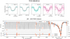 |
Fig. 5 Light curves and RV data of TOI-6628. We show the best juliet joint-fit model in black. FEROS RVs are shown in blue and HARPS RVs are shown in red. The top panel shows the TESS light curves, the bottom left panel shows the RV time series, and the bottom right panel shows the RV phase-folded data. The black line in the O-C of the RV time series is centered around zero for comparison with the RV residuals after the best-fit model substraction. |
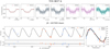 |
Fig. 6 Light curves and RV data of TOI 3837. We show the best juliet joint-fit model in black. FEROS RVs are shown in blue and HARPS RVs are shown in red. The top panel shows the TESS light curves, the bottom left panel shows the RV time series, and the bottom right panel shows the RV phase-folded data. The black line in the O-C of the RV time series is centered around zero to compare with the RV residuals after the best-fit model substraction. |
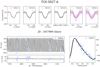 |
Fig. 7 Light curves and RV data of TOI-5027. We show the best juliet joint-fit model in black. FEROS RVs are shown in blue. The top panel shows the TESS light curves, the bottom left panel shows the RV time series, and the bottom right panel shows the RV phase-folded data. The black line in the O-C of the RV time series is centered around zero for comparison with the RV residuals after the best-fit model substraction. |
4.1.3 TOI-5027 b
The dataset used for the global modeling of TOI-5027 b consists of three TESS light curves: one LCOGT light curve with a cadence of 2 min, one OMES-RiDK500 light curve with a cadence of 1 min, and 16 FEROS RVs. The light curves of TESS sectors 12, 39, and 66 have a cadence of 30 min, 10 min, and 2 min, respectively. FEROS RVs are modeled with a Keplerian eccentric orbit. The best-fit model is shown in black in Fig. 7, and the phase-folded light curves are shown in the central-right panel in Fig. 2. The planet parameters of TOI-5027 b are shown in Table 6.
Our analysis indicates that TOI-5027 b is a WJ with a mass MP = 2.02±0.13 MJ and a radius  RJ, yielding a mean density
  (g/cm3). It orbits its host star every 10.24368±0.00001 days in an eccentric orbit with
  and has a time-averaged equilibrium temperature of
  .
.
4.1.4 TOI-2328 b
The dataset used for the orbit modeling of TOI-2328 b consists of six TESS light curves, one CHAT light curve with a 2 min cadence, one LCOGT light curve with a 1 min cadence, one Hazelwood light curve with a 3 min cadence, one OMES- CDK600 light curve with a cadence of 30 sec, 16 FEROS RVs, 12 HARPS RVs, and 12 PFS RVs. The TESS light curves from sectors 1 and 13 are from the 30 min cadence TESS-SPOC data, while the TESS light curves from sectors 27, 28, 39, 67, and 68 are from the 2 min cadence TESS-SPOC PDC-SAP data (Caldwell et al. 2020). We included a linear term to model the effect of air mass in the light curve from Hazelwood. FEROS, HARPS, and PFS RVs are modeled with a Keplerian eccentric orbit. The best-fit model is shown in black in Fig. 8, and the phase-folded light curves are shown in the bottom right panel in Fig. 2. The planet parameters of TOI-2328 b are shown in Table 6.
TOI-2328 b is a Saturn-like planet with a mass MP = 0.16±0.02 MJ, a radius  RJ, and a mean density of
  (g/cm3). It orbits its host star every 17.10197±0.00001 days in an orbit with
  and has a time-averaged equilibrium temperature of
  K.
K.
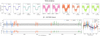 |
Fig. 8 Light curves and RV data of TOI-2328. We show the best juliet joint-fit model in black. FEROS RVs are shown in blue, HARPS RVs are shown in red, and PFS RVs are shown in green. The top panel shows the TESS light curves, the bottom left panel shows the RV time series, and the bottom right panel shows the RV phase-folded data. The black line in the O-C of the RV time series is centered around zero for comparison with the RV residuals after the best-fit model substraction. The black circles in the RV phase-folded data show the binned RV data. |
5 Interior modeling
We generate interior models with the GAS gianT modeL for Interiors (GASTLI, Acuña et al. 2024, 2021). The equations of hydrostatic equilibrium, adiabatic temperature, Gauss’s theorem, and conservation of mass are solved along a 1D grid that represents the planet radius from the center up to the interior boundary at a pressure of 1000 bar. The grid is stratified into two layers: a core composed of a 1:1 rock and water mixture and an envelope constituted by H/He and water. The amount of water in the envelope is determined by the envelope metallicity, log([Fe/H]P), which is a free parameter. We used up-to-date equations of state (EOSs) to compute the density of silicates (Lyon 1992; Miguel et al. 2022), water (Mazevet et al. 2019; Haldemann et al. 2020), and H/He (Chabrier & Debras 2021; Howard & Guillot 2023). The interior model is coupled with a grid of cloud-free, self-consistent atmospheric models obtained with petitCODE (Mollière et al. 2015, 2017) to calculate the atmospheric temperature. The conversion from atmospheric metallicity to the metal-mass fraction, Zenv , which is required to calculate the density of the H/He-water mixture, is done by assuming chemical equilibrium with easyCHEM (Mollière et al. 2017). We ensure convergence of the interior radius and boundary temperature with an iterative algorithm (Acuña et al. 2021).
Finally, the total radius is calculated by adding the atmospheric thickness at the transit pressure (Lopez & Fortney 2014; Grimm et al. 2018; Mousis et al. 2020, 20 mbar), to the converged interior radius. The age of the planet of each interior model is calculated by solving the equation of thermal cooling,  , where Tint is the internal (or intrinsic) temperature (Fortney et al. 2007; Acuña et al. 2024). This and the planet’s equilibrium temperature are free parameters in our atmospheric grid. In addition to the planet mass and the envelope metallicity, the core-mass fraction (CMF) is a free variable that parameterizes the composition of the planet. The bulk metal-mass fraction of the planet, which comprises the metals contained in both the core and the envelope, can then be obtained as Zplanet = CMF + (1-CMF) ×Zenv.
We used a Markov chain Monte Carlo (MCMC) algorithm (emcee; Foreman-Mackey et al. 2013) to sample the posterior distribution. We adopted uniform priors for CMF (0 to 0.99), log(Fe/H) (−2 to 2, equivalent to subsolar to 100 × solar), and Tint (50 to 400 K), while the planet mass, MP , follows a Gaussian prior according to its observed mean and uncertainties (see Table 6). The log-likelihood is calculated with the squared residuals of the observable parameters (mass, radius, and age) as indicated in Dorn et al. (2015) and Acuña et al. (2021). Our grid of atmospheric models spans an equilibrium temperature from 100 to 1000 K; hence, for TOI-5027 b and TOI-3837 b, we adopted Teq = 1000 K. This is close enough to the equilibrium temperature of TOI-5027 b (1056 K) to have negligible effects on its metal-mass content estimate. For TOI-3837 b, this difference of 180 K in equilibrium temperature can entail a difference in the core-mass fraction of ∆CMF = 0.02. This small correction should be taken into account when comparing our estimate for TOI-3837 b with other interior models.
Table 11 shows the mean and uncertainties obtained in the interior structure retrievals. Given the degeneracy between CMF and envelope metallicity, which can only be solved by atmospheric characterization data, the interior models span a wide range of atmospheric metallicities. However, our analysis allows us to determine the bulk metal-mass fraction of the planet. TOI-3837 b has a metal content between that of Jupiter and Saturn, and TOI-6628 b is compatible with a Saturn-like composition. In contrast, TOI-5027 b and TOI-2328 b have bulk metal-mass fractions between Saturn’s (Zplanet ∼ 0.20) and Neptune’s (Zplanet = 0.80–0.90) values (Miguel & Vazan 2023). To compare the bulk metal content of these four planets with the extrasolar, warm gas-giant population, we show the mass-bulk metallicity trend in Fig. 9. The star’s metal content is computed with the metallicity of their respective host star, [Fe/H] (Table 4), as Zstar = 0.0152 × 10[Fe/H]. We calculated the uncertainties of the Zplanet/Zstar ratio in Fig. 9 by sampling the MCMC’s posterior distribution function of the planet’s bulk metal-mass fraction, by assuming a Gaussian distribution of the stellar [Fe/H] using the bootstrap method. TOI-2328 b and TOI-3837 b closely follow the exoplanet mass-bulk metallicity trend, indicating that these two planets probably formed via core accretion (Thorngren et al. 2016). TOI-6628 b’s metal-content ratio is compatible with Jupiter uncertainties. In contrast, TOI-5027 b is slightly more metal-rich than the 1σ estimate of the exoplanet trend. This indicates that TOI-5027 b may have formed by accreting both pebbles and vapor-enriched gas during the runaway accretion phase (Helled & Morbidelli 2021; Bitsch & Mah 2023).
For comparison, we also computed interior models for the three gas giants presented here (TOI-6628 b, TOI-3837 b, and TOI-5027 b) using the modules for experiments in stellar astrophysics (MESA; Paxton et al. 2011). For this, we mainly followed the implementation presented in Jones et al. (2024), but here we computed models with all of the heavy elements in the core and a pure H/He gaseous envelope. In addition, we estimated the density of the core using the equation of state presented in Hubbard & Marley (1989), using a 7:3 mixture (in mass) of rock and ice. The resulting models that better reproduce the position of these planets in the age-radius diagram are presented in Fig. 10, and the corresponding planet metallicity and heavyelement enrichment with respect to the host star are listed in Table 11. The results obtained by these two sets of models agree well within 1σ.
Interior modeling parameters of TOI-6628 b, TOI-3837 b, TOI-5027 b, and TOI-2328 b, calculated using GASTLI and MESA.
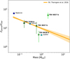 |
Fig. 9 Mass-bulk metallicity diagram. To compare the composition relative to the host star of the four newly discovered warm gas giants, we show the Solar System gas and ice giants, as well as the fit obtained by Thorngren et al. (2016) for a sample of extrasolar warm gas giants. |
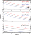 |
Fig. 10 Position of TOI-6628 b, TOI-3837 b, and TOI-5027 b in the age-radius diagram (black dot in the upper, middle, and lower panels, respectively). Planet evolutionary models with different core masses and densities are over-plotted. |
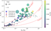 |
Fig. 11 Planet radius as a function of the planet mass for the population of warm giant planets (P > 10 days), color-coded by equilibrium temperature. The size of the circles scales with the transit spectroscopy metric (TSM; Kempton et al. 2018). Dashed red lines correspond to bulk densities of 0.1, 1, and 10 g cm−3. |
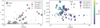 |
Fig. 12 Distribution of eccentricities and planet radius as a function of orbital period for planets with periods up to 200 days. Left panel: orbital eccentricity as a function of orbital period for the population of transiting planets. TOI-6028 b and TOI-5027 b are among the few discovered high-eccentricity planets. Right panel: planet radius versus orbital period diagram for the population of giant planets (MP>0.1 MJ), color-coded by planet mass. The size of the circles scales with the TSM. The four systems presented in this study belong to the population of long-period planets with P > 10 days. |
6 Discussion
TOI-6628 b, TOI-3837 b, TOI-5027 b, and TOI-2328 b are four giant planets with masses between 0.1 and two Jupiter masses, orbital periods between ten and 20 days, and predicted time- averaged equilibrium temperatures below 1200 K. Figure 11 shows the population of well-characterized transiting exoplanets in the planet’s mass-planet radius plane, which is size-coded by the transit spectroscopy metric (TSM; Kempton et al. (2018)) and color-coded on Teq. The TSM values of TOI-6628 b, TOI- 5027 b, TOI-3837 b, and TOI-2328 b are 14.2±3.6, 24.1±6.2, 14.1±5.4, and 75.4±11.9.
Given their distance to their host star, irradiation levels in the surface of the planet from the host star should be mild enough to neglect proximity effects in the study of the planet’s internal bulk structure. Their time-averaged surface temperatures are all below 1200 K, and their incident flux is below 2×10⁸ erg/s. Because of this, WJs generally have radii similar to or below 1 RJ , while hot Jupiters have radii well above the predictions according to classical planetary structural models (Zapolsky & Salpeter 1969).
Three of our targets orbit their host star in eccentric orbits, the exception being TOI-2328 b. We highlight the case of TOI- 6628 b, which has a measured eccentricity of  , and the case of TOI-5027 b, which has a measured eccentricity of
  . They are among the few planets orbiting in high- eccentricity orbits. In the case of TOI-3837 b, we measured an eccentricity of
  . The ∆log evidence between the eccentric and non-eccentric models is 4.8, providing moderate to strong evidence supporting the eccentric solution. Winn & Fabrycky (2015) predicted a wide distribution of warm giant’s eccentricities, as opposed to HJs circular orbits. Our findings provide additional evidence for theoretical expectations. The left panel in Fig. 12 shows the population of well-characterized transiting exoplanets with periods shorter than 200 days in the period-eccentricity plane, size-coded by planetary mass, and the right panel in Fig. 12 shows the population of giant planets with MP > 0.1 MJ in the planet period-radius plane, color-coded by planetary mass and size coded by TSM. All four planets lie in the region of this plane that is still sparsely populated. Only 5% of the total population of giant planets detected so far have eccentricities larger than 0.5, and TOI-6628 b is one of them. They belong to a growing population of WJs with planetary radii close to 1 RJ orbiting their host stars with periods longer than ten days. Moreover, about 2/3 of the total population of transiting exoplanets have circular orbits with e <0.1. Hence, TOI-6628 b, TOI-3837 b, and TOI-5027 b belong to an emerging population of still rare warm giants in rather eccentric orbits.
Long-term trends in RV residuals of TOI-6628 b, TOI- 3837 b, and TOI-5027 b suggest the presence of possible outer companions. However, it is not possible to constrain the properties of the outer companion with the current data. A long-term RV follow-up campaign should provide better constraints on observed linear trends.
Orbital obliquities measured using the Rossiter–McLaughlin effect (R–M) can be a powerful tool to constrain warm-Jupiter migration theories (Petrovich & Tremaine 2016). Taking into account an impact parameter b of zero, the upper limits for the amplitudes of the R-M effect for TOI-6628 b, TOI-3837 b, TOI-5027 b, and TOI-2328 b are 31.3±5.4 m/s, 23.4 m/s±4.6, 54.5±6.8 m/s, and 27.1 m/s±5.0, respectively. This makes this set of planets well-suited targets for the measurement of the projected angle between the stellar and orbital angular momenta. By studying the obliquity distribution of the growing population of WJs, we will be able to further understand giant planet formation and evolution.
Planet interior models suggest that the TOI-6628 b, TOI- 3837 b, TOI-5027 b, and TOI-2328 b internal structure most likely consists of an icy and rocky core and a gaseous envelope composed mainly of hydrogen and helium, providing supporting evidence to the core accretion theory of planet formation. While MESA models consider the metals to be concentrated in the core, GASTLI considers the metals to be mixed in the envelope. MESA models incorporate the effect of stellar evolution in the planet’s interior structure, which can play an important role in the case of stars that are evolving off the main sequence; this increases their luminosity, which seems to be the case for TOI- 3837. Both GASTLI and MESA models are consistent and in excellent agreement within the uncertainties.
7 Conclusions
We report the discovery of planetary companions orbiting TOI-6628, TOI-3837, TOI-5027, and TOI-2328. TOI-6628 b has a mass of 0.74 ± 0.06 MJ and orbits its host star every 18.18424 ± 0.00001 days in an eccentric orbit with  . TOI-3837 b has a mass of 0.59±0.05 MJ and an eccentricity of
  . TOI-5027 b is the most massive of the four, with a mass of 2.02±0.13 MJ, and it has an eccentricity of
  . TOI-2328 b has a mass of 0.16±0.02 MJ and orbits its host star in circular orbit. By building up a sample of fully characterized WJs, it will be possible to study the orbital parameter distributions and provide further constraints to planetary formation and evolution models.
Data availability
Tables A.1, A.2, A.3, and A.4 are available in electronic form at CDS via anonymous ftp to cdsarc.cds.unistra.fr (130.79.128.5) or via https://cdsarc.cds.unistra.fr/viz-bin/cat/J/A+A/694/A268.
Acknowledgements
M.T.P. acknowledges the support of Fondecyt-ANID fellowship no. 3210253 and ASTRON-0037. A.J., R.B. and V.S. acknowledge support from ANID – Millennium Science Initiative – ICN12_009 and AIM23-0001. R.B. acknowledges support from FONDECYT Project 1241963. A.J. acknowledges support from FONDECYT project 1210718. The results reported herein benefitted from collaborations and/or information exchange within NASA’s Nexus for Exoplanet System Science (NExSS) research coordination network sponsored by NASA’s Science Mission Directorate under Agreement No. 80NSSC21K0593 for the program “Alien Earths”.
Appendix A Activity indices
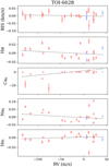 |
Fig. A.1 Stellar activity indices plotted as a function of the RV for TOI 6628. The gray dashed line show the best linear fit to the data. The red points correspond to HARPS measurements and the blue points correspond to FEROS measurements. |
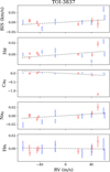 |
Fig. A.2 Stellar activity indices plotted as a function of the RV for TOI 3837. The gray dashed line show the best linear fit to the data. The red points correspond to HARPS measurements and the blue points correspond to FEROS measurements. |
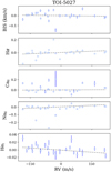 |
Fig. A.3 Stellar activity indices plotted as a function of the RV for TOI 5027. The gray dashed line show the best linear fit to the data. The blue points correspond to FEROS measurements. |
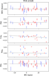 |
Fig. A.4 Stellar activity indices plotted as a function of the RV for TOI 2328. The gray dashed line show the best linear fit to the data. The red points correspond to HARPS measurements and the blue points correspond to FEROS measurements. |
References
- Acuña, L., Deleuil, M., Mousis, O., et al. 2021, A&A, 647, A53 [NASA ADS] [CrossRef] [EDP Sciences] [Google Scholar]
- Acuña, L., Kreidberg, L., Zhai, M., & Mollière, P. 2024, A&A, 688, A60 [NASA ADS] [CrossRef] [EDP Sciences] [Google Scholar]
- Albrecht, S., Winn, J. N., Johnson, J. A., et al. 2012, ApJ, 757, 18 [NASA ADS] [CrossRef] [Google Scholar]
- Andretta, V., Busà, I., Gomez, M. T., & Terranegra, L. 2005, A&A, 430, 669 [NASA ADS] [CrossRef] [EDP Sciences] [Google Scholar]
- Bakos, G., Noyes, R. W., Latham, D. W., et al. 2006, in Tenth Anniversary of 51 Peg-b: Status of and Prospects for Hot Jupiter Studies, eds. L. Arnold, F. Bouchy, & C. Moutou, 184 [Google Scholar]
- Barclay, T., Pepper, J., & Quintana, E. V. 2018, ApJS, 239, 2 [Google Scholar]
- Bitsch, B., & Mah, J. 2023, A&A, 679, A11 [NASA ADS] [CrossRef] [EDP Sciences] [Google Scholar]
- Boisse, I., Moutou, C., Vidal-Madjar, A., et al. 2009, A&A, 495, 959 [NASA ADS] [CrossRef] [EDP Sciences] [Google Scholar]
- Borucki, W. J. 2017, Proc. Am. Philos. Soc., 161, 38 [Google Scholar]
- Brahm, R., Jordán, A., Hartman, J., & Bakos, G. 2017, MNRAS, 467, 971 [NASA ADS] [Google Scholar]
- Brahm, R., Jordán, A., & Espinoza, N. 2017, PASP, 129, 034002 [Google Scholar]
- Brahm, R., Espinoza, N., Jordán, A., et al. 2019, AJ, 158, 45 [Google Scholar]
- Brahm, R., Nielsen, L. D., Wittenmyer, R. A., et al. 2020, AJ, 160, 235 [Google Scholar]
- Brahm, R., Ulmer-Moll, S., Hobson, M. J., et al. 2023, AJ, 165, 227 [NASA ADS] [CrossRef] [Google Scholar]
- Bressan, A., Marigo, P., Girardi, L., et al. 2012, MNRAS, 427, 127 [NASA ADS] [CrossRef] [Google Scholar]
- Brown, T. M., Baliber, N., Bianco, F. B., et al. 2013, PASP, 125, 1031 [Google Scholar]
- Burnham, K., & Anderson, D. 2003, Model Selection and Multimodel Inference: A Practical Information-Theoretic Approach (Springer New York) [Google Scholar]
- Butler, R. P., Marcy, G. W., Williams, E., et al. 1996, PASP, 108, 500 [Google Scholar]
- Caldwell, D. A., Tenenbaum, P., Twicken, J. D., et al. 2020, RNAAS, 4, 201 [NASA ADS] [Google Scholar]
- Cameron, A. G. W. 1978, Moon Planets, 18, 5 [Google Scholar]
- Castelli, F., & Kurucz, R. L. 2003, in Modelling of Stellar Atmospheres, 210, eds. N. Piskunov, W. W. Weiss, & D. F. Gray, A20 [NASA ADS] [Google Scholar]
- Chabrier, G., & Debras, F. 2021, ApJ, 917, 4 [NASA ADS] [CrossRef] [Google Scholar]
- Chatterjee, S., Ford, E. B., Matsumura, S., & Rasio, F. A. 2008, ApJ, 686, 580 [NASA ADS] [CrossRef] [Google Scholar]
- Collins, K. A., Kielkopf, J. F., Stassun, K. G., & Hessman, F. V. 2017, AJ, 153, 77 [Google Scholar]
- Crane, J. D., Shectman, S. A., & Butler, R. P. 2006, in Ground-based and Airborne Instrumentation for Astronomy, 6269, eds. I. S. McLean & M. Iye, International Society for Optics and Photonics (SPIE), 626931 [NASA ADS] [CrossRef] [Google Scholar]
- Crane, J. D., Shectman, S. A., Butler, R. P., Thompson, I. B., & Burley, G. S. 2008, in Ground-based and Airborne Instrumentation for Astronomy II, 7014, eds. I. S. McLean, & M. M. Casali, International Society for Optics and Photonics (SPIE), 701479 [Google Scholar]
- Crane, J. D., Shectman, S. A., Butler, R. P., et al. 2010, in Ground-based and Airborne Instrumentation for Astronomy III, 7735, eds. I. S. McLean, S. K. Ramsay, & H. Takami, International Society for Optics and Photonics (SPIE), 773553 [NASA ADS] [Google Scholar]
- Dawson, R. I., & Johnson, J. A. 2018, ARA&A, 56, 175 [Google Scholar]
- Dong, J., Huang, C. X., Dawson, R. I., et al. 2021, ApJS, 255, 6 [NASA ADS] [CrossRef] [Google Scholar]
- Dorn, C., Khan, A., Heng, K., et al. 2015, A&A, 577, A83 [NASA ADS] [CrossRef] [EDP Sciences] [Google Scholar]
- Duncan, D. K., Vaughan, A. H., Wilson, O. C., et al. 1991, ApJS, 76, 383 [Google Scholar]
- Espinoza, N., Hartman, J. D., Bakos, G. A., et al. 2019, AJ, 158, 63 [NASA ADS] [CrossRef] [Google Scholar]
- Espinoza, N., Kossakowski, D., & Brahm, R. 2019, MNRAS, 490, 2262 [Google Scholar]
- Foreman-Mackey, D., Hogg, D. W., Lang, D., & Goodman, J. 2013, PASP, 125, 306 [Google Scholar]
- Fortney, J. J., Marley, M. S., & Barnes, J. W. 2007, ApJ, 659, 1661 [Google Scholar]
- Fressin, F., Torres, G., Charbonneau, D., et al. 2013, ApJ, 766, 81 [NASA ADS] [CrossRef] [Google Scholar]
- Fulton, B. J., Petigura, E. A., Blunt, S., & Sinukoff, E. 2018, PASP, 130, 044504 [Google Scholar]
- Gaia Collaboration (Prusti, T., et al.) 2016, A&A, 595, A1 [NASA ADS] [CrossRef] [EDP Sciences] [Google Scholar]
- Gaia Collaboration (Brown, A. G. A., et al.) 2018, A&A, 616, A1 [NASA ADS] [CrossRef] [EDP Sciences] [Google Scholar]
- Gaia Collaboration (Vallenari, A., et al.) 2023, A&A, 674, A1 [NASA ADS] [CrossRef] [EDP Sciences] [Google Scholar]
- Gill, S., Wheatley, P. J., Cooke, B. F., et al. 2020, ApJ, 898, L11 [Google Scholar]
- Gomes da Silva, J., Santos, N. C., Bonfils, X., et al. 2011, A&A, 534, A30 [NASA ADS] [CrossRef] [EDP Sciences] [Google Scholar]
- Grimm, S. L., Demory, B.-O., Gillon, M., et al. 2018, A&A, 613, A68 [NASA ADS] [CrossRef] [EDP Sciences] [Google Scholar]
- Guerrero, N. M., Seager, S., Huang, C. X., et al. 2021, ApJS, 254, 39 [NASA ADS] [CrossRef] [Google Scholar]
- Haldemann, J., Alibert, Y., Mordasini, C., & Benz, W. 2020, A&A, 643, A105 [NASA ADS] [CrossRef] [EDP Sciences] [Google Scholar]
- Hartman, J. D., Bakos, G. Á., Bayliss, D., et al. 2019, AJ, 157, 55 [Google Scholar]
- Hatzes, A. P., & Rauer, H. 2015, ApJ, 810, L25 [Google Scholar]
- Helled, R., & Morbidelli, A. 2021, in ExoFrontiers; Big Questions in Exoplanetary Science, ed. N. Madhusudhan (IOP), 12 [Google Scholar]
- Hobson, M. J., Brahm, R., Jordán, A., et al. 2021, AJ, 161, 235 [NASA ADS] [CrossRef] [Google Scholar]
- Hobson, M. J., Trifonov, T., Henning, T., et al. 2023, AJ, 166, 201 [NASA ADS] [CrossRef] [Google Scholar]
- Howard, S., & Guillot, T. 2023, A&A, 672, L1 [NASA ADS] [CrossRef] [EDP Sciences] [Google Scholar]
- Howell, S. B., Sobeck, C., Haas, M., et al. 2014, PASP, 126, 398 [Google Scholar]
- Huang, C., Wu, Y., & Triaud, A. H. M. J. 2016, ApJ, 825, 98 [NASA ADS] [CrossRef] [Google Scholar]
- Huang, C. X., Vanderburg, A., Pál, A., et al. 2020a, RNAAS, 4, 204 [Google Scholar]
- Huang, C. X., Vanderburg, A., Pál, A., et al. 2020b, RNAAS, 4, 206 [NASA ADS] [Google Scholar]
- Hubbard, W. B., & Marley, M. S. 1989, Icarus, 78, 102 [Google Scholar]
- Jeffreys, H. 1939, Theory of Probability (Oxford University Press) [Google Scholar]
- Jenkins, J. M., Twicken, J. D., McCauliff, S., et al. 2016, SPIE Conf. Ser., 9913, 99133E [Google Scholar]
- Jones, M. I., Brahm, R., Espinoza, N., et al. 2019, A&A, 625, A16 [NASA ADS] [CrossRef] [EDP Sciences] [Google Scholar]
- Jones, M. I., Reinarz, Y., Brahm, R., et al. 2024, A&A, 683, A192 [NASA ADS] [CrossRef] [EDP Sciences] [Google Scholar]
- Jordán, A., Brahm, R., Espinoza, N., et al. 2019, AJ, 157, 100 [Google Scholar]
- Jordán, A., Brahm, R., Espinoza, N., et al. 2020, AJ, 159, 145 [Google Scholar]
- Kass, R. E., & Raftery, A. E. 1995, J. Am. Statist. Assoc., 90, 773 [CrossRef] [Google Scholar]
- Kaufer, A., Stahl, O., Tubbesing, S., et al. 1999, The Messenger, 95, 8 [Google Scholar]
- Kempton, E.M. R., Bean, J. L., Louie, D. R., et al. 2018, PASP, 130, 114401 [CrossRef] [Google Scholar]
- Kossakowski, D., Espinoza, N., Brahm, R., et al. 2019, MNRAS, 490, 1094 [NASA ADS] [CrossRef] [Google Scholar]
- Kovács, G., Zucker, S., & Mazeh, T. 2002, A&A, 391, 369 [Google Scholar]
- Kozai, Y. 1962, AJ, 67, 591 [Google Scholar]
- Kreidberg, L. 2015, batman: BAsic Transit Model cAlculatioN in Python, Astrophysics Source Code Library [record ascl:1510.002] [Google Scholar]
- Kunimoto, M., & Daylan, T. 2021, TESS Science conference 2, 62 [NASA ADS] [Google Scholar]
- Kunimoto, M., Huang, C., Tey, E., et al. 2021, RNAAS, 5, 234 [NASA ADS] [Google Scholar]
- Kunimoto, M., Tey, E., Fong, W., et al. 2022, RNAAS, 6, 236 [NASA ADS] [Google Scholar]
- Lidov, M. L. 1962, Planet. Space Sci., 9, 719 [Google Scholar]
- Lopez, E. D., & Fortney, J. J. 2014, ApJ, 792, 1 [Google Scholar]
- Lyon, S. P. 1992, Los Alamos National Laboratory report LA-UR-92-3407 [Google Scholar]
- Madhusudhan, N., Amin, M. A., & Kennedy, G. M. 2014, ApJ, 794, L12 [Google Scholar]
- Mandushev, G., Torres, G., Latham, D. W., et al. 2005, ApJ, 621, 1061 [NASA ADS] [CrossRef] [Google Scholar]
- Mayor, M., Marmier, M., Lovis, C., et al. 2011, arXiv e-prints [arXiv:1109.2497] [Google Scholar]
- Mayor, M., Pepe, F., Queloz, D., et al. 2003, The Messenger, 114, 20 [NASA ADS] [Google Scholar]
- Mazevet, S., Licari, A., Chabrier, G., & Potekhin, A. Y. 2019, A&A, 621, A128 [NASA ADS] [CrossRef] [EDP Sciences] [Google Scholar]
- McCully, C., Volgenau, N. H., Harbeck, D.-R., et al. 2018, in Software and Cyberinfrastructure for Astronomy V, 10707, eds. J. C. Guzman, & J. Ibsen, International Society for Optics and Photonics (SPIE), 107070K [NASA ADS] [Google Scholar]
- Méndez, A., & Rivera-Valentín, E. G. 2017, ApJ, 837, L1 [Google Scholar]
- Miguel, Y., & Vazan, A. 2023, Remote Sensing, 15, 681 [NASA ADS] [CrossRef] [Google Scholar]
- Miguel, Y., Bazot, M., Guillot, T., et al. 2022, A&A, 662, A18 [NASA ADS] [CrossRef] [EDP Sciences] [Google Scholar]
- Mollière, P., van Boekel, R., Dullemond, C., Henning, T., & Mordasini, C. 2015, ApJ, 813, 47 [Google Scholar]
- Mollière, P., van Boekel, R., Bouwman, J., et al. 2017, A&A, 600, A10 [Google Scholar]
- Mollière, P., Molyarova, T., Bitsch, B., et al. 2022, ApJ, 934, 74 [CrossRef] [Google Scholar]
- Mousis, O., Deleuil, M., Aguichine, A., et al. 2020, ApJ, 896, L22 [NASA ADS] [CrossRef] [Google Scholar]
- Munari, U., Henden, A., Frigo, A., et al. 2014, AJ, 148, 81 [NASA ADS] [CrossRef] [Google Scholar]
- Noyes, R. W., Weiss, N. O., & Vaughan, A. H. 1984, ApJ, 287, 769 [Google Scholar]
- Paxton, B., Bildsten, L., Dotter, A., et al. 2011, ApJS, 192, 3 [Google Scholar]
- Petrovich, C., & Tremaine, S. 2016, ApJ, 829, 132 [NASA ADS] [CrossRef] [Google Scholar]
- Pollack, J. B., Hubickyj, O., Bodenheimer, P., et al. 1996, Icarus, 124, 62 [NASA ADS] [CrossRef] [Google Scholar]
- Queloz, D., Henry, G. W., Sivan, J. P., et al. 2001, A&A, 379, 279 [NASA ADS] [CrossRef] [EDP Sciences] [Google Scholar]
- Rafikov, R. R. 2005, ApJ, 621, L69 [Google Scholar]
- Rasio, F. A., & Ford, E. B. 1996, Science, 274, 954 [Google Scholar]
- Ricker, G. R., Winn, J. N., Vanderspek, R., et al. 2015, J. Astron. Telesc. Instrum. Syst., 1, 014003 [Google Scholar]
- Santerne, A., Moutou, C., Tsantaki, M., et al. 2016, A&A, 587, A64 [NASA ADS] [CrossRef] [EDP Sciences] [Google Scholar]
- Schlecker, M., Kossakowski, D., Brahm, R., et al. 2020, AJ, 160, 275 [Google Scholar]
- Schlichting, H. E. 2014, ApJ, 795, L15 [Google Scholar]
- Shatsky, N., Belinski, A., Dodin, A., et al. 2020, in Ground-Based Astronomy in Russia. 21st Century, eds. I. I. Romanyuk, I. A. Yakunin, A. F. Valeev, & D. O. Kudryavtsev, 127 [CrossRef] [Google Scholar]
- Skrutskie, M. F., Cutri, R. M., Stiening, R., et al. 2006, AJ, 131, 1163 [NASA ADS] [CrossRef] [Google Scholar]
- Smith, J. C., Stumpe, M. C., Cleve, J. E. V., et al. 2012, PASP, 124, 1000 [NASA ADS] [CrossRef] [Google Scholar]
- Speagle, J. S. 2020, MNRAS, 493, 3132 [Google Scholar]
- Stevenson, D. 1982, Planet. Space Sci., 30, 755 [NASA ADS] [CrossRef] [Google Scholar]
- Stumpe, M. C., Smith, J. C., Cleve, J. E. V., et al. 2012, PASP, 124, 985 [NASA ADS] [CrossRef] [Google Scholar]
- Stumpe, M. C., Smith, J. C., Catanzarite, J. H., et al. 2014, PASP, 126, 100 [Google Scholar]
- Tayar, J., Claytor, Z. R., Huber, D., & van Saders, J. 2022, ApJ, 927, 31 [NASA ADS] [CrossRef] [Google Scholar]
- Thorngren, D. P., Fortney, J. J., Murray-Clay, R. A., & Lopez, E. D. 2016, ApJ, 831, 64 [NASA ADS] [CrossRef] [Google Scholar]
- Tokovinin, A. 2018, PASP, 130, 035002 [Google Scholar]
- Trifonov, T., Brahm, R., Espinoza, N., et al. 2021, AJ, 162, 283 [NASA ADS] [CrossRef] [Google Scholar]
- Trifonov, T., Brahm, R., Jordán, A., et al. 2023, AJ, 165, 179 [NASA ADS] [CrossRef] [Google Scholar]
- Twicken, J. D., Catanzarite, J. H., Clarke, B. D., et al. 2018, PASP, 130, 064502 [Google Scholar]
- Udalski, A., Szewczyk, O., Zebrun, K., et al. 2002, Acta Astron., 52, 317 [Google Scholar]
- Walsh, K. J., Morbidelli, A., Raymond, S. N., O’Brien, D. P., & Mandell, A. M. 2011, Nature, 475, 206 [Google Scholar]
- Winn, J. N., & Fabrycky, D. C. 2015, ARA&A, 53, 409 [Google Scholar]
- Wu, Y., & Lithwick, Y. 2011, ApJ, 735, 109 [Google Scholar]
- Zapolsky, H. S., & Salpeter, E. E. 1969, ApJ, 158, 809 [Google Scholar]
- Zechmeister, M., & Kürster, M. 2018, GLS: Generalized Lomb-Scargle periodogram, Astrophysics Source Code Library [record ascl:1807.019] [Google Scholar]
- Ziegler, C., Tokovinin, A., Briceño, C., et al. 2020, AJ, 159, 19 [Google Scholar]
Based on data collected from the NASA exoplanet archive.
Leaving [Fe/H] as a free parameters led to the same results.
Our four target stars are too faint to provide a reliable measure of the  on the individual spectra.
All Tables
∆LogZ values of the four different models we tested with respect to the model with the highest logZ.
Prior parameter distributions and median value of the posterior distributions of the fitted parameters of the joint transit and RV analysis of TOI-6628 b.
Prior parameter distributions and median value of the posterior distributions of the fit parameters of the joint transit and RV analysis of TOI-3837 b.
Prior parameter distributions and median value of the posterior distributions of the fit parameters of the joint transit and RV analysis of TOI-5027 b.
Prior parameter distributions and median value of the posterior distributions of the fit parameters of the joint transit and RV analysis of TOI-2328 b.
Interior modeling parameters of TOI-6628 b, TOI-3837 b, TOI-5027 b, and TOI-2328 b, calculated using GASTLI and MESA.
All Figures
|
Fig. 1 TESS target pixel files (TPF) of TOI-6628, TOI-3837, TOI-5027, and TOI-2328. We show the aperture mask used in the light-curve measurement with red striped squares. We indicate the Gaia (Gaia Collaboration 2018) magnitudes of the targets and surrounding stars. |
| In the text | |
|
Fig. 2 Phase-folded light curve of TOI-6628.01, TOI-3837.01, TOI-5027.01, and TOI-2328.01. The best model is shown in black. |
| In the text | |
|
Fig. 3 High-resolution images of TOI-3837 and TOI-5027. |
| In the text | |
|
Fig. 4 Periodograms of photometric and spectroscopic data of TOI-6628, TOI-3837, TOI-5027, and TOI-2328, respectively. The horizontal red dashed line corresponds to the GLS 1% false alarm probability and the blue vertical dashed line marking the planet period. |
| In the text | |
|
Fig. 5 Light curves and RV data of TOI-6628. We show the best juliet joint-fit model in black. FEROS RVs are shown in blue and HARPS RVs are shown in red. The top panel shows the TESS light curves, the bottom left panel shows the RV time series, and the bottom right panel shows the RV phase-folded data. The black line in the O-C of the RV time series is centered around zero for comparison with the RV residuals after the best-fit model substraction. |
| In the text | |
|
Fig. 6 Light curves and RV data of TOI 3837. We show the best juliet joint-fit model in black. FEROS RVs are shown in blue and HARPS RVs are shown in red. The top panel shows the TESS light curves, the bottom left panel shows the RV time series, and the bottom right panel shows the RV phase-folded data. The black line in the O-C of the RV time series is centered around zero to compare with the RV residuals after the best-fit model substraction. |
| In the text | |
|
Fig. 7 Light curves and RV data of TOI-5027. We show the best juliet joint-fit model in black. FEROS RVs are shown in blue. The top panel shows the TESS light curves, the bottom left panel shows the RV time series, and the bottom right panel shows the RV phase-folded data. The black line in the O-C of the RV time series is centered around zero for comparison with the RV residuals after the best-fit model substraction. |
| In the text | |
|
Fig. 8 Light curves and RV data of TOI-2328. We show the best juliet joint-fit model in black. FEROS RVs are shown in blue, HARPS RVs are shown in red, and PFS RVs are shown in green. The top panel shows the TESS light curves, the bottom left panel shows the RV time series, and the bottom right panel shows the RV phase-folded data. The black line in the O-C of the RV time series is centered around zero for comparison with the RV residuals after the best-fit model substraction. The black circles in the RV phase-folded data show the binned RV data. |
| In the text | |
|
Fig. 9 Mass-bulk metallicity diagram. To compare the composition relative to the host star of the four newly discovered warm gas giants, we show the Solar System gas and ice giants, as well as the fit obtained by Thorngren et al. (2016) for a sample of extrasolar warm gas giants. |
| In the text | |
|
Fig. 10 Position of TOI-6628 b, TOI-3837 b, and TOI-5027 b in the age-radius diagram (black dot in the upper, middle, and lower panels, respectively). Planet evolutionary models with different core masses and densities are over-plotted. |
| In the text | |
|
Fig. 11 Planet radius as a function of the planet mass for the population of warm giant planets (P > 10 days), color-coded by equilibrium temperature. The size of the circles scales with the transit spectroscopy metric (TSM; Kempton et al. 2018). Dashed red lines correspond to bulk densities of 0.1, 1, and 10 g cm−3. |
| In the text | |
|
Fig. 12 Distribution of eccentricities and planet radius as a function of orbital period for planets with periods up to 200 days. Left panel: orbital eccentricity as a function of orbital period for the population of transiting planets. TOI-6028 b and TOI-5027 b are among the few discovered high-eccentricity planets. Right panel: planet radius versus orbital period diagram for the population of giant planets (MP>0.1 MJ), color-coded by planet mass. The size of the circles scales with the TSM. The four systems presented in this study belong to the population of long-period planets with P > 10 days. |
| In the text | |
|
Fig. A.1 Stellar activity indices plotted as a function of the RV for TOI 6628. The gray dashed line show the best linear fit to the data. The red points correspond to HARPS measurements and the blue points correspond to FEROS measurements. |
| In the text | |
|
Fig. A.2 Stellar activity indices plotted as a function of the RV for TOI 3837. The gray dashed line show the best linear fit to the data. The red points correspond to HARPS measurements and the blue points correspond to FEROS measurements. |
| In the text | |
|
Fig. A.3 Stellar activity indices plotted as a function of the RV for TOI 5027. The gray dashed line show the best linear fit to the data. The blue points correspond to FEROS measurements. |
| In the text | |
|
Fig. A.4 Stellar activity indices plotted as a function of the RV for TOI 2328. The gray dashed line show the best linear fit to the data. The red points correspond to HARPS measurements and the blue points correspond to FEROS measurements. |
| In the text | |
Current usage metrics show cumulative count of Article Views (full-text article views including HTML views, PDF and ePub downloads, according to the available data) and Abstracts Views on Vision4Press platform.
Data correspond to usage on the plateform after 2015. The current usage metrics is available 48-96 hours after online publication and is updated daily on week days.
Initial download of the metrics may take a while.