| Issue |
A&A
Volume 698, June 2025
|
|
|---|---|---|
| Article Number | A112 | |
| Number of page(s) | 18 | |
| Section | Catalogs and data | |
| DOI | https://doi.org/10.1051/0004-6361/202452431 | |
| Published online | 06 June 2025 | |
sunset: A database of synthetic atmospheric-escape transmission spectra for nearly every transiting planet
1
Anton Pannekoek Institute for Astronomy, University of Amsterdam,
Science Park 904,
1098
XH
Amsterdam,
The Netherlands
2
Center for Astrophysics | Harvard & Smithsonian,
60 Garden Street, MS-16,
Cambridge,
MA
02138,
USA
★ Corresponding author: This email address is being protected from spambots. You need JavaScript enabled to view it.
Received:
30
September
2024
Accepted:
18
April
2025
Abstract
Studying atmospheric escape from exoplanets can provide important clues about the formation and evolution of exoplanets. Observational evidence of atmospheric escape has been obtained through transit spectroscopy in strong spectral lines of various atomic species. In recent years, the number of exoplanets that have been targeted in this way has grown rapidly, mainly by observations of the metastable helium triplet. Even with this larger sample of exoplanets, many aspects of atmospheric escape are still not fully understood, such as the role of the stellar high-energy spectrum and planetary magnetic field, highlighting the need for additional observations. This work aims to identify the best targets for observations in various spectral lines. Using the atmospheric escape code sunbather, we calculated a synthetic transmission spectrum of nearly every transiting exoplanet currently known. This database of spectra, named sunset, is publicly available. We introduce metrics that predict spectral line observability, which allow for swift identification of the most favorable targets. By analyzing the complete set of spectra from a demographic perspective, we find that the atmospheric mass-loss rate does not explain all the spread in the strength of various spectral lines, suggesting that a nondetection does not immediately rule out an escaping atmosphere. Some lines also do not correlate very strongly with one another, emphasizing the benefits of observing multiple spectral lines. Our model spectra show only a modest correlation between the X-ray and extreme UV flux and the helium line strength, affirming that the absence of such a trend found by observational works is not necessarily surprising. A direct comparison between our synthetic spectra and the sample of observed metastable helium spectra shows that they are generally consistent within the large model uncertainties. This suggests, in general, that photoevaporation is able to explain the current metastable helium census.
Key words: methods: numerical / catalogs / planets and satellites: atmospheres / planets and satellites: physical evolution
© The Authors 2025
 Open Access article, published by EDP Sciences, under the terms of the Creative Commons Attribution License (https://creativecommons.org/licenses/by/4.0), which permits unrestricted use, distribution, and reproduction in any medium, provided the original work is properly cited.
This article is published in open access under the Subscribe to Open model. This email address is being protected from spambots. You need JavaScript enabled to view it. to support open access publication.
1 Introduction
Thousands of exoplanets have been discovered to date. The majority of them have been discovered with the transit and radial velocity methods, which are biased toward finding planets at short orbital distances. Therefore, most of the currently known exoplanets receive high amounts of stellar radiation, which can cause their atmospheres to escape (e.g., Yelle 2004; Koskinen et al. 2007). For some planets, the escape process can be so efficient that it strips a significant part of the planet’s mass. This is theorized to be one of the mechanisms responsible for shaping the sub-Jovian desert and radius valley (Szabó & Kiss 2011; Kurokawa & Nakamoto 2014; Fulton et al. 2017; Owen & Lai 2018; Ho & Van Eylen 2023). High-gravity and furtherout planets are believed to be more stable against transformative mass-loss. In addition to the evolutionary implications, studying atmospheric escape can also provide valuable insights into physical phenomena such as planetary magnetic fields and stellar winds (Bourrier & Lecavelier des Etangs 2013; Vidotto & Bourrier 2017; Carolan et al. 2021; Gupta et al. 2023), which are known to affect atmospheric mass loss in solar system planets (e.g., Gronoff et al. 2020).
Ongoing atmospheric escape can be studied with transit spectroscopy in spectral lines that form in the low-density, high-altitude layers of the atmosphere, such as the hydrogen Lyman-α line (e.g., Vidal-Madjar et al. 2003; Lecavelier des Etangs et al. 2010; Bourrier et al. 2018), the metastable helium triplet (e.g., Oklopčić & Hirata 2018; Spake et al. 2018; Allart et al. 2018; Nortmann et al. 2018), and various lines from metals, mostly in the UV (e.g., Vidal-Madjar et al. 2004; Sing et al. 2019; García Muñoz et al. 2021). In recent years, the number of planets that have been targeted in the metastable helium triplet has grown rapidly. It has thus started to become feasible to interpret them in a statistical sense, in addition to the more in-depth interpretation and modeling of individual planets. Several works have already searched for correlations between the observed helium signals and system parameters that should influence atmospheric escape, such as age, high-energy radiation, stellar spectral type, and planetary gravity (Zhang et al. 2023a; Bennett et al. 2023; Krishnamurthy & Cowan 2024; Orell-Miquel et al. 2024). The expected preference of helium detections around K-type host stars has been observationally supported (Oklopčić 2019; Krishnamurthy & Cowan 2024; Orell-Miquel et al. 2024). However, the expected dependence on the X-ray and extreme UV (EUV; together XUV) flux is somewhat unclear, as Bennett et al. (2023) found a correlation with the stellar ![Mathematical equation: $\[R_{H K}^{\prime}\]$](/articles/aa/full_html/2025/06/aa52431-24/aa52431-24-eq1.png) activity indicator, while no correlation with the stellar age has been found (Krishnamurthy & Cowan 2024; Orell-Miquel et al. 2024), although both parameters are related to the stellar XUV flux.
activity indicator, while no correlation with the stellar age has been found (Krishnamurthy & Cowan 2024; Orell-Miquel et al. 2024), although both parameters are related to the stellar XUV flux.
To better determine the role that each of these system parameters plays, a larger sample of atmospheric escape observations is needed. In this regard, the upcoming high-resolution spectrograph NIGHT will prove extremely useful, as it will be dedicated to metastable helium triplet observations of more than a hundred exoplanets (Farret Jentink et al. 2024b; Farret Jentink et al. 2024a). At the same time, it will be helpful to increase the sample of exoplanets with observations in other spectral lines that trace atmospheric escape. Other spectral lines will have a different dependence on the same system parameters (e.g., Linssen & Oklopčić 2023), so by observing these lines, we may get a more comprehensive view of the physics that govern atmospheric escape rather than the physics underlying the metastable helium triplet specifically.
One of the main goals of this work is to identify exoplanets that are potentially good targets in upcoming observations of various spectral lines that trace atmospheric escape. Our approach is based on using sunbather (Linssen et al. 2024), an open-source code for modeling the spectral signatures of escaping atmospheres. We have calculated a synthetic transmission spectrum of the upper atmosphere of almost every transiting exoplanet currently known. The synthetic spectra are freely available to the community in our online database called sunset1 and can be used to inform observational campaigns.
This paper is structured as follows. In Sect. 2, we describe our numerical modeling, including the input system parameters, stellar SED templates, and free model parameters. We also provide an overview of the assumptions and sources of uncertainty in our models. In Sect. 3, we describe our resulting output spectra and explore correlations between various system parameters and spectral line strengths. In Sect. 4, we compare our synthetic spectra to the sample of planets with metastable helium observations. In Sect. 5, we summarize our work and our findings. Additionally, in Appendix B, we list the most promising observational targets for a selection of spectral lines.
2 Methods
2.1 System parameters
To calculate the transmission spectra of the transiting exoplanet population, we started by downloading the planetary parameters from the NASA Exoplanet Archive2. We used the Composite Planet Data from January 16, 2024. The composite data combines multiple publications into a single set of parameters per planet, resulting in relatively high completeness, though not all parameters are internally consistent. From the initial database of 5569 planets, we first selected the 4182 planets that are transiting and noncontroversial and then selected the 4144 planets (hereafter, our “initial population”) that have a reported value for all the parameters that we needed to produce model spectra. Required are the planet mass (Mp), radius (Rp), and semimajor axis (a), as well as the stellar mass (M*), radius (R*), and a value for either the star’s spectral type or effective temperature (Teff, which we then used as a proxy for the spectral type, assuming the star is on the main sequence). For many planets, some of these parameters have considerable uncertainties, which propagated into our model results. Instead of filtering out such planets beforehand, we proceeded to model every planet possible, and we provide tailored warnings for individual planets that have large uncertainties on the used parameters.
2.2 Stellar SED templates
One of the most important yet uncertain factors affecting the planet’s mass-loss rate, upper atmospheric structure, and transit spectrum is the host star’s spectral energy distribution (SED), particularly at XUV wavelengths. These SEDs are not readily available for the great majority of exoplanets. Therefore, we used the SEDs of proxy stars with a similar spectral type. Our sample of stellar SEDs mainly consists of spectra from the MUSCLES, Mega-MUSCLES, and MUSCLES Extension surveys (France et al. 2016; Youngblood et al. 2016; Loyd et al. 2016; Wilson et al. 2021; Behr et al. 2023). These surveys yielded a collection of panchromatic spectra of stars ranging from F- to M-type with measured X-ray and reconstructed EUV components. For some spectral types, mainly between M1 and M4, there are multiple stars in the survey with a similar spectral type but varying levels of XUV flux (FXUV). For planets in our initial population with such a host spectral type, it is generally not clear which SED template is most appropriate to use. Therefore, starting from the full collection of 34 available MUSCLES spectra, we selected a subset of 18 stars with non-overlapping spectral types. We selected stars with intermediate levels of XUV flux, thereby aiming to exclude relatively active or inactive stars (see lower panel of Fig. 1). In addition to the MUSCLES spectra, we also included the SED of the Sun, based on measurements by the TIMED (Woods et al. 2005) and SORCE (Rottman 2005) spacecrafts, due to the high data quality of this spectrum. The way the solar spectrum was constructed is described in more detail in Sect. 3 of Linssen et al. (2024). Finally, to accommodate earlier-type stars, we added the spectra of an A7 and an A0 star. These are based on the model spectra with effective temperatures of 7500 K and 10 000 K, respectively, from Fossati et al. (2018). The XUV flux of the A7 star is from a solar spectrum scaled up by a factor of three. The full sample of used SEDs with their spectral types and effective temperatures are listed in Table 1 and shown in Fig. 1.
In our initial planet population, there are 944 planets with a reported host spectral type, and we assigned the SED with the closest spectral type to them. The remaining planets all have a reported stellar effective temperature, and we assigned the SED with the closest effective temperature to them. This is more or less the simplest approach possible, as it does not factor in the age and activity levels of the planet host star or, more generally, the possible variety in the XUV flux level of the star.
2.3 Model parameters
Our simulations were performed using the 1D atmospheric escape code sunbather (Linssen et al. 2024). This code first models the upper atmosphere as an isothermal Parker wind (Parker 1958; Lamers & Cassinelli 1999) using the p-winds (dos Santos et al. 2022) and Cloudy (Ferland et al. 2017; Chatzikos et al. 2023) codes. Afterward, it refines the temperature to a nonisothermal profile. The use of Cloudy then enables the calculation of transmission spectra spanning a large wavelength range and including spectral lines from many different elements.
In addition to the system parameters and the SED, three main free parameters are required to run sunbather: the mass-loss rate ![Mathematical equation: $\[(\dot{M})\]$](/articles/aa/full_html/2025/06/aa52431-24/aa52431-24-eq2.png) , the temperature (T0), and the atmospheric composition. To choose the mass-loss rate of each planet, we used the parametrization given in Appendix A of Caldiroli et al. (2022). They ran a grid of models with the ATES code (Caldiroli et al. 2021), which simulates the launching of photoevaporative outflows by modeling photoionization of hydrogen-helium atmospheres and predicts the corresponding mass-loss rates. Their analytic formula for the mass-loss rate is calculated for a hydrogen-helium atmosphere (with relative abundances set to He/H=0.083 in number density), expressed as the energy-limit escape formula, where the parametrization takes place in the form of a non-constant efficiency factor ηeff. However, we clarify that these mass-loss rates should not be thought of as being energy limited. ATES does not strictly model outflows that are in the energy-limited regime, and the code is perfectly able to transition into a recombination-limited outflow, for example. In such a case, the efficiency factor would simply become much lower than one. Their parametrization of the mass-loss rate comes from fitting a complex functional form to the output mass-loss rates of the model grid, with dependencies on Rp, Mp, a, M*, and FXUV. This analytic fit is precise to within a factor ~1.5, but can only safely be assumed to be valid in their explored parameter range: 102 ≲ FXUV/ρp ≲ 106 and 1012.17 ≲ Kϕ ≲ 1013.29, where ρp is the planet’s mean density, K is the Roche-lobe correction factor from Erkaev et al. (2007), and ϕ = GMp/Rp is the planet’s gravitational potential. Unfortunately, there are quite many planets in our initial population that fall outside of these bounds. Most of these are cases where Kϕ is below its lower bound (and often FXUV/ρp too), which is a part of the parameter space where the efficiency varies only slowly with both quantities (see Fig. A.1 of Caldiroli et al. 2022), so that we are still relatively confident in applying the parametrization outside of these bounds. There is also a smaller number of planets where Kϕ is above its upper bound, where the efficiency dependency is strong. Our adopted efficiency (and hence mass-loss rate) for these planets will be much more inaccurate. These high-gravity planets represent the non-inflated Jovian population. However, the efficiency already tends to ηeff ≲ 10−4 at this upper boundary, leading to very low mass-loss rates. At low mass-loss rates, sunbather often fails to converge (the reasons for this are discussed in more detail below), so that most of these planets did not make it to our successfully simulated “final population” anyway. In Fig. 2, we show the mass-loss rates we obtained for the planets in our initial population.
, the temperature (T0), and the atmospheric composition. To choose the mass-loss rate of each planet, we used the parametrization given in Appendix A of Caldiroli et al. (2022). They ran a grid of models with the ATES code (Caldiroli et al. 2021), which simulates the launching of photoevaporative outflows by modeling photoionization of hydrogen-helium atmospheres and predicts the corresponding mass-loss rates. Their analytic formula for the mass-loss rate is calculated for a hydrogen-helium atmosphere (with relative abundances set to He/H=0.083 in number density), expressed as the energy-limit escape formula, where the parametrization takes place in the form of a non-constant efficiency factor ηeff. However, we clarify that these mass-loss rates should not be thought of as being energy limited. ATES does not strictly model outflows that are in the energy-limited regime, and the code is perfectly able to transition into a recombination-limited outflow, for example. In such a case, the efficiency factor would simply become much lower than one. Their parametrization of the mass-loss rate comes from fitting a complex functional form to the output mass-loss rates of the model grid, with dependencies on Rp, Mp, a, M*, and FXUV. This analytic fit is precise to within a factor ~1.5, but can only safely be assumed to be valid in their explored parameter range: 102 ≲ FXUV/ρp ≲ 106 and 1012.17 ≲ Kϕ ≲ 1013.29, where ρp is the planet’s mean density, K is the Roche-lobe correction factor from Erkaev et al. (2007), and ϕ = GMp/Rp is the planet’s gravitational potential. Unfortunately, there are quite many planets in our initial population that fall outside of these bounds. Most of these are cases where Kϕ is below its lower bound (and often FXUV/ρp too), which is a part of the parameter space where the efficiency varies only slowly with both quantities (see Fig. A.1 of Caldiroli et al. 2022), so that we are still relatively confident in applying the parametrization outside of these bounds. There is also a smaller number of planets where Kϕ is above its upper bound, where the efficiency dependency is strong. Our adopted efficiency (and hence mass-loss rate) for these planets will be much more inaccurate. These high-gravity planets represent the non-inflated Jovian population. However, the efficiency already tends to ηeff ≲ 10−4 at this upper boundary, leading to very low mass-loss rates. At low mass-loss rates, sunbather often fails to converge (the reasons for this are discussed in more detail below), so that most of these planets did not make it to our successfully simulated “final population” anyway. In Fig. 2, we show the mass-loss rates we obtained for the planets in our initial population.
The second free parameter of sunbather is the temperature. To determine which value to use, we performed a “self-consistency check” where we compared the chosen T0 to the nonisothermal temperature profile that the code solves for. Such a self-consistency check has been performed before, albeit using different criteria (Linssen et al. 2022; Linssen & Oklopčić 2023; Linssen et al. 2024). Here, we searched for the value of T0 that is equal to the maximum temperature of its nonisothermal profile ![Mathematical equation: $\[(\hat{T})\]$](/articles/aa/full_html/2025/06/aa52431-24/aa52431-24-eq3.png) . Such a value of T0 is unique, meaning there is only one possible value (at a given mass-loss rate). Multiple simulations with different values of T0 are typically needed to find this “self-consistent” T0. In concrete terms, we started the search for T0 of each planet with a simulation at T0 = 10 000 K. We then extracted
. Such a value of T0 is unique, meaning there is only one possible value (at a given mass-loss rate). Multiple simulations with different values of T0 are typically needed to find this “self-consistent” T0. In concrete terms, we started the search for T0 of each planet with a simulation at T0 = 10 000 K. We then extracted ![Mathematical equation: $\[\hat{T}\]$](/articles/aa/full_html/2025/06/aa52431-24/aa52431-24-eq4.png) from the nonisothermal profile and started a new simulation at T0 equal to
from the nonisothermal profile and started a new simulation at T0 equal to ![Mathematical equation: $\[(\hat{T}+T_{0}) / 2\]$](/articles/aa/full_html/2025/06/aa52431-24/aa52431-24-eq5.png) . We were satisfied when the temperatures are self-consistent to within
. We were satisfied when the temperatures are self-consistent to within ![Mathematical equation: $\[|\hat{T}-T_{0}|<300 \mathrm{~K}\]$](/articles/aa/full_html/2025/06/aa52431-24/aa52431-24-eq6.png) . Afterwards, we only used the “self-consistent” model and discarded the other ones, so that we obtained one atmospheric model per planet.
. Afterwards, we only used the “self-consistent” model and discarded the other ones, so that we obtained one atmospheric model per planet.
Since sunbather involves the use of Cloudy, it is subject to the limitations of Cloudy. At high densities (roughly ≳1015 g s−1), Cloudy often fails to converge, as the code was not designed for such conditions. In general, such high densities are reached for high-gravity planets, and at low T0. The latter is the reason that we used a self-consistency criterion based on the maximum of the nonisothermal temperature profile, since this criterion yields the highest values of T0 for which one may reasonably argue that the temperature is self-consistent. In this way, we were able to successfully simulate more planets, but it does admittedly introduce some bias toward lower density, higher temperature and velocity outflows. We quantify this bias in Appendix C. Using this criterion, the highest gravity planets still reach atmospheric densities above what Cloudy can handle, and we thus failed to simulate them. Fortunately, these high-gravity planets are also expected to be stable against atmospheric escape and therefore are not very interesting targets in the context of our research.
The final free model parameter is the atmospheric composition. We used a solar composition for all planets. We motivate this by the fact that the mass-loss rate predictions from ATES are based on hydrogen-helium only simulations, and would not be valid for high-metallicity outflows. We still added metals at solar abundances to our simulations, because they do not affect the atmospheric structure very significantly at these relatively low abundances (e.g., Zhang et al. 2022; Kubyshkina et al. 2024; Linssen et al. 2024), but already produce strong lines in the transit spectrum that we aim to investigate. The assumption of a solar metallicity atmosphere may be particularly unrealistic for sub-Neptune exoplanets. Various sub-Neptunes have recently been shown to have high-metallicity atmospheres (e.g., Kempton et al. 2023; Benneke et al. 2024; Wogan et al. 2024). It is not yet completely clear how the lower-atmospheric metallicity as constrained with the James Webb Space Telescope (JWST) by these works relates to the upper-atmospheric metallicity. Under various assumptions, Zhang et al. (2025) found a 100 times solar metallicity escaping atmosphere for the mini-Neptune TOI836 b, indicating that the upper atmosphere of small exoplanets may indeed also be rich in metals. A high metallicity outflow is expected to result in a lower mass-loss rate, a different atmospheric structure, and hence a different transit spectrum (e.g., Zhang et al. 2022, 2025; Linssen et al. 2024). However, running models with different compositions for each exoplanet is beyond the scope of this work. If the assumption of solar composition turns out to be unrealistic for most sub-Neptune planets, the simulations performed here are still valuable from a theoretical perspective.
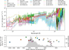 |
Fig. 1 Top: stellar spectral energy distribution templates used in this work. The A0 and A7 spectra are based on the work of Fossati et al. (2018), the solar spectrum is from the TIMED and SORCE missions (Woods et al. 2005; Rottman 2005), and the rest of the spectra are from the MUSCLES survey (France et al. 2016; Youngblood et al. 2016; Loyd et al. 2016; Wilson et al. 2021; Behr et al. 2023). Bottom: integrated XUV flux (λ < 911 Å) of each SED as a function of the effective temperature of the star (scatter points; see also Table 1). Small black points indicate SEDs in the MUSCLES database that we do not use. The grey histogram (read from the right y-axis) shows the host star effective temperatures of the initial planet population. Planets are assigned the SED template of the closest stellar spectral type. If the spectral type is not reported, the SED template of the star with the closest effective temperature is assigned. |
Spectral types and effective temperatures of the stars used in our SED sample.
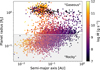 |
Fig. 2 Mass-loss rates of the initial planet population calculated from the analytical approximation of Caldiroli et al. (2022, Appendix A). The mass-loss rate is parametrized as a function of Rp, Mp, a, M*, and FXUV, based on the output of the first-principle 1D photoevaporation code ATES (Caldiroli et al. 2021). The shaded lower region indicates planets with radii <2.5RE, which are potentially rocky. We do produce spectra for these planets that we include in sunset, but do not include them when analyzing our final planet population in Sect. 3. |
2.4 Calculation of transmission spectra
With mass-loss rates calculated and an algorithm in place to determine the temperature, we started the sunbather simulations for all 4144 planets. 220 of them failed because of high-density problems with Cloudy, while another 26 failed because of instabilities in the sunbather algorithm that solves the nonisothermal temperature profile. We successfully simulated the remaining 3898 planets and continued to calculate their transmission spectra. We used the planet’s own impact parameter, or 0 if it is not reported. The spectra were calculated at mid-transit, with no stellar center-to-limb variations. The wavelength grid runs from 911 Å to 11 000 Å at a high spectral resolution of R ~ 400 000. A total of 12 191 spectral lines from various elements are present in this wavelength region. sunbather includes spectral line broadening due to natural broadening, thermal broadening, and the Doppler shift from the line-of-sight component of the outflow velocity. The velocity component due to the tidally locked rotation of the planet is not included. All gas within the atmospheric domain of [1Rp, 8Rp] was included (the part of it that covers the stellar disk), irrespective of the Roche radius. This choice is somewhat arbitrary and can be debated. Beyond the Roche radius, our 1D model most certainly does not capture the geometry of the escaping material. However, since escaping gas does not simply disappear at the Roche radius, we opted to include gas beyond it, to allow for the existence of material in tails and streams contributing to the line formation. Lines that generally form below the Roche radius are not very affected by this choice, while lines that form at high altitudes are more uncertain (see Linssen & Oklopčić 2023 for an overview of the strongest lines and at which altitudes they form). In Appendix C, we provide an estimation of the uncertainty in our spectral line strengths due to the extent of the computational domain.
2.5 Uncertainties and warnings
Having described our modeling approach, we here provide a concise overview of the numerous uncertainties in our methods. Some of these uncertainties apply to most or all planets, and they have to do with choices and assumptions in our modeling framework. These overall uncertainties include:
The planet parameters are often collected from multiple sources, which are potentially not mutually consistent.
The XUV flux received by practically every planet is highly uncertain. We use template spectra from proxy host stars. These spectra may not be representative of the true flux received by the planet.
The planet is assumed to have an atmosphere. This assumption may be invalid for rocky exoplanets.
The atmospheric composition may be different from solar. Especially sub-Neptune exoplanets could host high-metallicity upper atmospheres.
The upper atmosphere may not be well described by a 1D Parker wind with a mass-loss rate as predicted by ATES, for example when atmospheric escape is not driven by photo-evaporation or when there are significant day-to-nightside differences, magnetic fields, stellar wind interactions, etc.
The chosen T0-value may be inappropriate. The criterion to choose its value by requiring self-consistency with the maximum temperature in the nonisothermal profile is somewhat arbitrary.
The transmission spectra are made without stellar center-to-limb darkening. Limb-darkening, or limb-brightening at farUV (FUV) wavelengths (Schlawin et al. 2010), could have a minor effect.
In addition to these methodological uncertainties, there are additional uncertainties or limiting factors that only apply to specific planets, typically because one or more of the input parameters are not well constrained. These include (the quoted planet numbers only include the successfully simulated planets in the sunset database):
Molecules are present at non-negligible abundances in the Cloudy simulation, which affects the atmospheric structure but is ignored by sunbather (seven planets).
The reported eccentricity is not a true value but an upper or lower limit (204 planets), the planet has eccentricity larger than 0.1 (296 planets), or the planet does not have a reported eccentricity (455 planets). sunbather assumes a circular orbit.
The planet radius is an upper or lower limit (two planets), the planet radius errors are larger than 10% (1723 planets), or the errors are not reported (429 planets).
The planet mass quoted in the NASA Exoplanet Archive is derived from the radius through a mass-radius relationship (2845 planets).
The planet mass is an upper or lower limit (82 planets), the planet mass errors are larger than 20% (359 planets), or the errors are not reported (three planets).
We calculated the semimajor axis from a reported a/R* value using the value of R* (221 planets), as opposed to using a directly reported value of a itself.
The semimajor axis errors are larger than 25% (39 planets), or the errors are not reported (2428 planets).
The stellar radius errors are larger than 25% (612 planets), or the errors are not reported (72 planets).
The stellar mass errors are larger than 25% (129 planets), or the errors are not reported (81 planets).
The planet transit impact parameter is an upper or lower limit (seven planets), or the planet transit impact parameter is unknown and we assumed 0 (135 planets).
The host star’s spectral type is more than two away from that of the used SED (e.g., F1 versus F4; 19 planets).
The host star’s spectral type is not reported and the effective temperature is used instead (3069 planets).
The host star’s effective temperature is more than 200 K away from that of the used SED (83 planets).
The stellar age is unknown. The star is potentially young with higher XUV flux (634 planets).
The star is younger than 1 Gyr, with potentially higher XUV flux (362 planets).
The FXUV/ρp value is outside of the formally valid bounds of the mass-loss rate parametrization (1490 planets).
The Kϕ value is outside of the formally valid bounds of the mass-loss rate parametrization (1963 planets).
The planet’s radius is smaller than 2.5 RE, which may indicate that it is a rocky planet, which likely does not have a primordial extended atmosphere (2189 planets). Otegi et al. (2020) find that the division between super-Earths and sub-Neptunes is best described by the composition line of water, roughly at a mean planet density of 3 g cm−3. However, the masses of most of the small exoplanets in our population are derived from the M-R relationship of Chen & Kipping (2017), so that imposing a density criterion is the same as using a radius criterion. Therefore, we prefer to simply use a radius criterion directly. According to Otegi et al. (2020), the transition from rocky to volatile-rich exoplanets occurs between 2–3 RE. We use an intermediate value of 2.5 RE to flag planets as potentially rocky.
Out of these different warnings, we consider the following to be relatively important: the mass is from a mass-radius relationship, no or large errors on the planet radius, planet mass, semimajor axis, or stellar mass, a used SED template that is more than two spectral types or 200 K effective temperature away from the host star, calculation of the mass-loss rate outside the validity bounds of the Caldiroli et al. (2022) formula, and planets with radii <2.5 RE that are potentially rocky. There are 326 exoplanets that have none of these warnings, and their model spectra are expected to be most accurate.
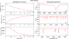 |
Fig. 3 Example of the publicly available1 output data products for the planet TOI-3235 b (simulated with sunbather; Linssen et al. 2024). Left column: upper atmospheric structure. Right column: zoom-in on various parts of the transmission spectrum. The full spectrum spans 911 Å to 11 000 Å at a spectral resolution of R ~ 400 000. It includes spectral lines from the 30 lightest elements (up until zinc). |
3 Results
Our output consists of atmospheric models (radial profiles of density, velocity, temperature, and mean particle mass) and transmission spectra of the 3898 successfully simulated exoplanets. These are freely available for download in the sunset database1. An example of the data products for a single exoplanet is shown in Fig. 3. Additionally, for each planet, we provide an information file with the specific warnings from the list in Sect. 2.5 that apply to it. For many planets, there are numerous serious warnings, and we very strongly caution against the blind use of such spectra. One could point out that it may not have been useful to proceed to simulate these planets. However, we prefer to obtain a database as large as possible, so that if needed, highly uncertain models can always be filtered out afterwards by inspecting their specific warnings.
In this section, we investigate trends in the sunset models. Before doing so, we filter out the potentially rocky planets (with Rp < 2.5 RE), as theoretical and observational work has indicated that these planets likely do not host primordially extended atmospheres (e.g., Venturini et al. 2020; Greene et al. 2023; Zieba et al. 2023; Burn et al. 2024). The remaining 1709 planets (hereafter called our “final population”), which we thus assume to be gaseous, can still have other serious warnings. This means that some of these spectra may indeed not prove realistic and useful for the real-world planets they were modeled after, but they are still useful for theoretically investigating the behavior of atmospheric escape properties and transit spectra, given these system parameters.
3.1 Bulk outflow parameter correlations
We start by investigating correlations between the various inand output parameters, in order to gain insight into the physics controlling atmospheric escape. In Fig. A.1, we show the correlations between five bulk quantities of the final planet population: the atmospheric temperature, the mass-loss rate, the planet gravitational potential, the XUV flux, and the escape parameter
![Mathematical equation: $\[\lambda=\frac{\phi}{v_s^2}=\frac{G M_p}{R_p} \frac{\bar{\mu}}{k T_0},\]$](/articles/aa/full_html/2025/06/aa52431-24/aa52431-24-eq7.png) (1)
(1)
where vs is the speed of sound, which is constant in the isothermal Parker wind model, and ![Mathematical equation: $\[\bar{\mu}\]$](/articles/aa/full_html/2025/06/aa52431-24/aa52431-24-eq8.png) is the averaged mean particle mass of the atmosphere (Lampón et al. 2020).
is the averaged mean particle mass of the atmosphere (Lampón et al. 2020).
When looking at the correlations in Fig. A.1, it is important to realize that ϕ comes directly from the NASA Exoplanet Archive parameters, and FXUV comes from the semimajor axis and the stellar SED template. Since the latter is chosen based on the reported stellar spectral type or effective temperature, the XUV flux should be considered an input parameter to our model, and its correlation with ϕ simply reveals the underlying observed planet population. The sub-Jovian desert can be vaguely distinguished from it, in the form of a lack of medium-gravity (log ϕ ≈ 12.5 erg g−1, i.e., hot Neptune-like) planets at high XUV flux (i.e., close-in). The mass-loss rate is also an input parameter for us, derived from some of the other system parameters, depending most strongly on FXUV and ϕ. This parametrization of the mass-loss rate is reflected in the correlation with these two parameters: ![Mathematical equation: $\[\dot{M} \propto F_{X U V}\]$](/articles/aa/full_html/2025/06/aa52431-24/aa52431-24-eq9.png) , but at high planet gravity,
, but at high planet gravity, ![Mathematical equation: $\[\eta_{\text {eff }} \propto \dot{M}\]$](/articles/aa/full_html/2025/06/aa52431-24/aa52431-24-eq10.png) drops dramatically.
drops dramatically.
Although the Parker wind temperature is an input parameter to sunbather, it can effectively be considered an output parameter of our model in this case, because we do not a priori know its value and instead solve for it using a self-consistency criterion (see Sect. 2.3). For this reason, it is interesting to see how the self-consistent value depends on the other parameters. By extension, this then also holds for λ because it is calculated from T0, ϕ, and ![Mathematical equation: $\[\bar{\mu}\]$](/articles/aa/full_html/2025/06/aa52431-24/aa52431-24-eq11.png) . From Fig. A.1, we see that T0 depends strongly on the gravitational potential: high-gravity planets develop hot outflows, while low-gravity planets develop relatively cold outflows. This behavior, here seen in the final planet population in a statistical sense, is in line with previous studies on atmospheric escape of individual planets (e.g., Salz et al. 2016; Caldiroli et al. 2021; Linssen et al. 2022). The temperature is naturally also seen to depend on the XUV flux, but the spread is larger than for the planet gravity. The temperature and mass-loss rate are also weakly correlated, where the temperature increases with the mass-loss rate, except at the highest temperatures that are reached at the lowest mass-loss rates. The latter sub-population represents the high-gravity planets, and it may therefore be more intuitive to state that T0 causally depends on ϕ and FXUV, and is only correlated with
. From Fig. A.1, we see that T0 depends strongly on the gravitational potential: high-gravity planets develop hot outflows, while low-gravity planets develop relatively cold outflows. This behavior, here seen in the final planet population in a statistical sense, is in line with previous studies on atmospheric escape of individual planets (e.g., Salz et al. 2016; Caldiroli et al. 2021; Linssen et al. 2022). The temperature is naturally also seen to depend on the XUV flux, but the spread is larger than for the planet gravity. The temperature and mass-loss rate are also weakly correlated, where the temperature increases with the mass-loss rate, except at the highest temperatures that are reached at the lowest mass-loss rates. The latter sub-population represents the high-gravity planets, and it may therefore be more intuitive to state that T0 causally depends on ϕ and FXUV, and is only correlated with ![Mathematical equation: $\[\dot{M}\]$](/articles/aa/full_html/2025/06/aa52431-24/aa52431-24-eq12.png) . However, this distinction is ultimately trivial, because
. However, this distinction is ultimately trivial, because ![Mathematical equation: $\[\dot{M}\]$](/articles/aa/full_html/2025/06/aa52431-24/aa52431-24-eq13.png) in turn is a function of ϕ and FXUV.
in turn is a function of ϕ and FXUV.
In principle, there are many more system parameters that are not shown in Fig. A.1, such as Rp, Mp, a, and M*. However, we found that rather than considering Rp and Mp individually, their combined value in the form of the planet gravity captures the outflow physics just as well. Similarly, FXUV captures the physics better than a. The stellar mass directly affects the stellar tidal gravity term, which in most cases only has a minor effect on the outflow physics. The stellar mass also indirectly affects the stellar spectral type and hence the used SED. For the bulk outflow properties that we consider in Fig. A.1, the total XUV flux is more important than the shape of the SED, and is already included. The SED shape has a stronger effect on the microphysics governing the line formation in the planetary transit spectrum and is considered in more detail in Sect. 3.2.
While we qualitatively established the dependence of the atmospheric temperature on the planet gravity and the XUV flux before, we find it useful to provide a rough quantitative estimate of this relation. To this end, we fit a simple power law through the final planet population T0-values, as a function of ϕ and FXUV. This fit is shown in Fig. 4, and is given by
![Mathematical equation: $\[T_0=1.63 \times 10^{-3}\left(\frac{\phi}{\mathrm{erg} \mathrm{~g}^{-1}}\right)^{0.492}\left(\frac{F_{X U V}}{\mathrm{erg} \mathrm{~cm}^{-2} \mathrm{~s}^{-2}}\right)^{0.0863} \mathrm{~K}.\]$](/articles/aa/full_html/2025/06/aa52431-24/aa52431-24-eq14.png) (2)
(2)
The fit still has considerable structured residuals. It generally underpredicts the temperature of planets with ϕ ≈ 12.5, and overpredicts the temperature of planets with ϕ ≳ 13. The residuals have a standard deviation of 881 K. The fit could not be improved by using a power law dependence on more or other system parameters. The functional form of the power law therefore seems to be the reason for the mediocre fit quality: the temperature does not truly depend on the gravitational potential and the XUV flux in this simple way. The power law fit is still useful, because it makes it easy to see how the temperature scales with the two parameters, at least to zeroth order. The T0-parametrization may furthermore find its use in swiftly estimating a prior to break the ![Mathematical equation: $\[T_{0}-\dot{M}\]$](/articles/aa/full_html/2025/06/aa52431-24/aa52431-24-eq15.png) -degeneracy that is often found in isothermal Parker-wind analyses of spectral line observations (e.g., Vissapragada et al. 2020; Paragas et al. 2021; Allart et al. 2023).
-degeneracy that is often found in isothermal Parker-wind analyses of spectral line observations (e.g., Vissapragada et al. 2020; Paragas et al. 2021; Allart et al. 2023).
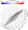 |
Fig. 4 Fit to the isothermal Parker wind temperature as a function of the planetary gravitational potential and received XUV flux. The final planet population (scatter points) is fitted with a power law (grey plane). The functional form is given by Eq. (2). The systematic residuals reveals that this functional form is not optimal, and particularly does not fully capture the dependence on the gravity. |
3.2 Spectral line strength correlations
We now investigate the correlations of various spectral lines. From the transmission spectrum of every planet, we extract the transit depth of the metastable helium triplet (10 833 Å), the calcium infrared triplet (8544 Å), the magnesium doublet (2796 Å), the iron UV2 multiplet (2383 Å), the carbon triplet (1336 Å), the oxygen triplet (1302 Å), and the silicon triplet (1265 Å). We selected these spectral lines because they trace a range of different elements, and all of them have been observed in exoplanetary systems (although the Si III λ 1265 detection of Linsky et al. 2010 has been contested by Ballester & Ben-Jaffel 2015). Even more atmospheric-escape tracers – such as Hα – have been observed, but they mainly probe the base of the outflow where the transition to hydrostatic equilibrium takes place. This part is not properly modeled in sunbather, and our predictions are expected to be less accurate in these lines (see Linssen & Oklopčić 2023 and Table C.1 therein). Similarly, the hydrogen Ly-α line is not accurately predicted because it is expected to be strongly shaped by the stellar environment. The correlations between the selected spectral lines and some of the bulk parameters are shown in Fig. A.2.
Most spectral lines correlate reasonably strongly with the mass-loss rate. For example, the Spearman’s ρ coefficient between the mass-loss rate and helium line strength is 0.67 (in log-log space). This means that the mass-loss rate certainly plays a role in setting the strength of the helium signal, but it does not account for all of the spread in predicted helium strengths. The physics governing the line formation are also important. Some of the planets with the highest mass-loss rates still show helium line strengths of only ~1%, which may go undetected in observations. We must therefore be careful not to simply equate helium (non)detections with atmospheric escape (non)detections, without conducting radiative transfer modeling for each system. The helium line strength furthermore does not correlate very strongly with the XUV flux (ρ = 0.48 in log-log space). This goes against the common assumption in the literature. Many works have searched for a trend in the observed exoplanet sample between the received XUV irradiation and the helium line depth (usually normalized by the scale height of the lower atmosphere) (e.g., Nortmann et al. 2018; Alonso-Floriano et al. 2019; Kasper et al. 2020; Zhang et al. 2021, 2023b; Fossati et al. 2022; Kirk et al. 2022; Poppenhaeger 2022; Orell-Miquel et al. 2022, 2024; Bennett et al. 2023; Zhang et al. 2023c; Guilluy et al. 2024; Krishnamurthy & Cowan 2024). Whether the correlation can be seen varies in these works, as the number of helium observations has grown over the years, but the most recent versions, based on the largest sample sizes, show no strong correlation. Fig. A.2 demonstrates that the absence of this correlation is actually in line with the expectations from our models. Our figure in principle shows this for the correlation between FXUV and the helium line strength, but the correlation is similar (ρ = 0.45) when we normalize the helium line strength with the atmospheric scale height, which most observational papers do. However, Fig. A.2 shows that the helium line strength anticorrelates more strongly with the stellar effective temperature (ρ = −0.64), which in this case can be considered a proxy for the shape of the SED. Specifically, the EUV/near-UV (NUV) flux ratio varies with stellar spectral type, and is known to influence the metastable helium abundance in the planet atmosphere (Oklopčić 2019). Our findings are in line with those of Ballabio & Owen (2025), who find that the helium line strength correlates more strongly with the XUV/FUV ratio than the XUV flux itself.
We move on to fit the helium line equivalent width (EW) as a function of various system parameters. Similar to our fit of the Parker wind temperature, we use a power law dependence, and find that the parameters giving the best fit are the planet mass and radius, the stellar radius, the XUV flux, and the ratio between the ground-state helium ionizing flux (FHe–ion) and metastable helium ionizing flux (FHe*–ion). We ignored the 275 planets with ϕ > 1013 g s−1, as in that regime, the dependence starts to deviate very strongly from a power law. We obtained
![Mathematical equation: $\[\begin{aligned}\mathrm{EW}_{\mathrm{He}}=154\left(\frac{R_p}{R_J}\right)^{3.14}\left(\frac{R_*}{R_{\odot}}\right)^{-1.78}\left(\frac{M_p}{M_J}\right)^{-0.990}\qquad\qquad\qquad \\ \cdot\left(\frac{F_{X U V}}{\mathrm{erg} ~\mathrm{cm}^{-2} \mathrm{s}^{-2}}\right)^{0.485}\left(\frac{F_{\mathrm{He}-\mathrm{ion}}}{F_{\mathrm{He}^*-\mathrm{ion}}}\right)^{0.498} \text {m\AA}.\end{aligned}\]$](/articles/aa/full_html/2025/06/aa52431-24/aa52431-24-eq16.png) (3)
(3)
We defined FHe–ion to be all wavelengths below 504 Å, and FHe*–ion to be between 911 and 2600 Å, but the fit is not sensitive to the chosen lower wavelength boundaries. The fit residuals have a standard deviation of a factor ~2. In this fit, the helium EW does depend on the XUV flux, despite our previous finding that these quantities are not strongly correlated in the final planet population. This likely means that variation in other system properties prevents a visible and strong correlation with the XUV flux alone.
Next, we phenomenologically identify and describe some trends we observe for certain spectral lines. It is beyond the scope of this paper to provide a microphysical explanation (in terms of the atomic structure, radiative transfer, etc.) for this behavior and we leave this for future work. The oxygen line strength shows the weakest correlation with the mass-loss rate (still ρ = 0.63) and XUV flux (ρ = 0.35) out of the different spectral lines. Even though the correlation coefficient with the stellar effective temperature is only −0.27, inspection of the figure reveals that the strongest oxygen line strengths are found around stars with Te f f ≲ 4000 K (i.e., M-dwarfs).
The carbon triplet correlates extremely strongly with the mass-loss rate (ρ = 0.93). The correlation is weaker – but still strong – with the XUV flux, which can influence the carbon line strength indirectly through the mass-loss rate, or directly through ionization of carbon to produce the absorbing C+. The former seems more likely, given the stronger correlation with the mass-loss rate. This suggests that the microphysics of this line are perhaps not very complex, and that the line simply becomes strong when there is a lot of escaping gas.
The magnesium, iron, and silicon lines show relatively strong correlation with the mass-loss rate. These lines additionally show modest correlation with the planet gravity. Lastly, the calcium infrared triplet is an interesting case, showing quite weak signals for most planets. However, there is a moderate correlation with the planet gravity, and the figure reveals that strong calcium infrared triplet signals are exclusively found around high-gravity planets (and mostly at relatively higher stellar effective temperatures). Therefore, the best chance to observe it seems to be on (ultra-)hot Jupiters orbiting early-type stars (in line with the findings of Linssen & Oklopčić 2023).
There is also insight to gain from the correlation between two spectral line depths. The lowest correlation is found between the metastable helium line and the calcium infrared triplet (ρ = 0.49). This seems to be the case due to the lines favoring different host star types. The lines thus favor complementary parts of the parameter space of planetary systems. When looking at the correlation between helium and the other spectral lines, we note that a strong helium signature typically also means that the other spectral lines are strong. However, planets with a weaker helium signature show a larger variety in metal line strengths of multiple orders of magnitude. All of these models consider the same solar composition atmosphere, implying that it is difficult to constrain the escaping atmospheric composition simply from an observed presence or absence of these lines: tailored planet models are needed to distinguish the effects of the hydrodynamics from the effects of the composition on the line-depth ratios. To a degree, the same reasoning holds for other line combinations that are not highly correlated, such as the carbon and oxygen lines.
In the metal-metal line correlations, we see that some combinations of lines are extremely correlated with ρ ≈ 1. Their line-depth ratio is apparently insensitive to differences in stellar flux and planetary parameters. The implication is that their line-depth ratio is instead an excellent tracer of the atmospheric composition and fractionation. The high correlation between the magnesium and iron lines may particularly be of observational interest, as they can be simultaneously observed using a single HST mode (Sing et al. 2019). In Appendix B, we provide a list of promising observational targets for each of the spectral lines discussed.
4 Comparison to the observed helium sample
4.1 Motivation
We now take a closer look at the results for the sample of exoplanets that have been observed in the metastable helium line. We are interested to see if our model predictions are generally consistent with the observational findings. There have been previous works with a similar goal, which typically search for correlations between the observed helium signal strength (or detection versus nondetection classification) and some of the physical parameters that are thought to influence atmospheric escape and helium observability, such as the stellar XUV flux (or a proxy thereof) and stellar spectral type. For example, Bennett et al. (2023) analyzed a sample of 37 planets, and found a positive correlation between the scale height-normalized helium depth and the stellar ![Mathematical equation: $\[R_{H K}^{\prime}\]$](/articles/aa/full_html/2025/06/aa52431-24/aa52431-24-eq17.png) activity indicator. They did not find a correlation with stellar age, metallicity, and rotation rate, nor with the planet’s surface gravity and semimajor axis. Krishnamurthy & Cowan (2024) analyzed the detection status of a sample of 57 planets, and found that most detections occurred around K- and G-type stars, and at semimajor axes between 0.03 and 0.08 AU. They also found that few detections occurred for small and low-mass planets, which they interpreted as these mature planets already having been stripped by atmospheric escape. They found no clear trends with stellar age and metallicity. Orell-Miquel et al. (2024) analyzed a sample of 70 planets with He I λ10 833, Hα, or Lyman-α observations. They found no correlation between the stellar age and the detection status of any of these lines, nor with the helium line equivalent width. Zhang et al. (2023a, Fig. 3) and Orell-Miquel et al. (2024, Fig. 7) also compared a proxy of the observed mass-loss rate (EWHe · R*), to an analytically estimated mass-loss rate (FXUV/ρXUV, where ρXUV is the mean density within the XUV photosphere radius). Both works did find a correlation between these proxies when considering the planets with positive helium detections. However, there were also many helium nondetections showing worse agreement with the fits.
activity indicator. They did not find a correlation with stellar age, metallicity, and rotation rate, nor with the planet’s surface gravity and semimajor axis. Krishnamurthy & Cowan (2024) analyzed the detection status of a sample of 57 planets, and found that most detections occurred around K- and G-type stars, and at semimajor axes between 0.03 and 0.08 AU. They also found that few detections occurred for small and low-mass planets, which they interpreted as these mature planets already having been stripped by atmospheric escape. They found no clear trends with stellar age and metallicity. Orell-Miquel et al. (2024) analyzed a sample of 70 planets with He I λ10 833, Hα, or Lyman-α observations. They found no correlation between the stellar age and the detection status of any of these lines, nor with the helium line equivalent width. Zhang et al. (2023a, Fig. 3) and Orell-Miquel et al. (2024, Fig. 7) also compared a proxy of the observed mass-loss rate (EWHe · R*), to an analytically estimated mass-loss rate (FXUV/ρXUV, where ρXUV is the mean density within the XUV photosphere radius). Both works did find a correlation between these proxies when considering the planets with positive helium detections. However, there were also many helium nondetections showing worse agreement with the fits.
The motivation for us to perform a seemingly similar exercise again is twofold. Firstly, the previous works compared the helium observations only to one or two of the system parameters at a time. While this exercise is certainly useful, it is typically not immediately clear whether the absence of an expected trend means that our theoretical understanding of atmospheric escape is lacking, or whether it can still be explained by variation in other system parameters that dilute the trend. With our approach, we compare directly with planet-specific models that aim to include most of these system parameters at once. This yields a more direct comparison of observation to theory – at least the physics included in our solar-composition 1D semiisothermal Parker wind model. Secondly, Fig. A.2 shows that according to our modeling, some of the presupposed correlations between the helium line strength and system parameters (specifically, the mass-loss rate, the planet gravity, and the XUV irradiation) are actually not very strong in the final planet population. We should thus perhaps not be very surprised that previous works generally did not find such strong correlations. This finding also strengthens the motivation for a direct comparison to planet-specific models.
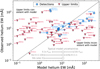 |
Fig. 5 Comparison between the observed and modeled EW of the metastable helium line for the near-complete planet sample as compiled in Orell-Miquel et al. (2024). The dotted line is x = y (i.e., complete agreement). The model uncertainties are very large. Rough estimates of the uncertainty due to the XUV flux (based on the scaling in Eq. (3)), the helium abundance (based on additional simulations of TOI-2018 b), and the metallicity (based on simulations of Linssen et al. 2024 of a generic hot Neptune planet) are indicated. An additional significant source of uncertainty is the shape of the stellar SED (specifically the ratio between EUV and NUV flux). Compared to the model uncertainties, observational uncertainties are very small (typically inside the size of the scatter marker) and therefore not shown. |
4.2 Comparison and interpretation
We started from the planet sample as compiled in Orell-Miquel et al. (2024), because it is currently the largest sample in the literature (but may still be incomplete). We focused on the 69 planets in the sample with helium observations, and extracted the helium line equivalent widths (or upper limits) from their Table M.15. From this sample, we did not have model spectra for four planets: TOI-1683 b is not in the NASA Exoplanet Archive, and our models for KELT-20 b, TOI-1431 b, and K2-77 b failed due to the Cloudy density limit described in Sect. 2.3. For the remaining 65 planets, we integrated the synthetic helium spectrum to obtain the EW, and plot these against the observed values in Fig. 5. We did not adopt the distinction between nonconclusive and nondetection measurements from Orell-Miquel et al. (2024), because their designation was based on a comparison to the energy-limited mass-loss rate, which is different from our used mass-loss rate. We caution that the model uncertainties are large, and may also vary significantly from planet to planet, depending on the precision on the input parameters.
Most of the planets with a positive helium detection have observed EWs relatively close to the model values (within a factor of a few). We consider these to be consistent given the large model uncertainties. The exceptions are HAT-P-32 b and HAT-P-67 b, which show almost two orders of magnitude higher absorption than predicted by the model. These planets have small Roche radii of 2.1 Rp and 2.6 Rp, respectively, and are therefore likely in an escape regime where the mass loss is significantly enhanced over what ATES predicted. The outflow geometry becomes highly non-spherical in this regime, and leading and trailing arms develop. This has indeed been observed for both planets (Czesla et al. 2022; Zhang et al. 2023c; Bello-Arufe et al. 2023; Gully-Santiago et al. 2024). These arms and the extra absorption in them are not captured by our model and could thus lead to the discrepancy. However, some of the other planets in the sample have small Roche radii as well, and using the same reasoning, our model would have underpredicted their absorption too. WASP-67 b, TOI-1807 b, WASP-52 b, HAT-P-57 b, KELT-9 b, LTT 9779 b, WASP-127 b, and WASP-177 b all have Roche radii smaller than 3Rp, which would lead to a stronger tension with the observed signals for some of these planets.
Most of the planets with helium nondetections have upper limits that are above or close to the model predictions, which we consider to be consistent. The planets in the bottom-right part of the figure are those that are most inconsistent, and they warrant individual consideration. These planets include the following:
The TRAPPIST-1 planets are all likely terrestrial instead of gaseous planets and are thus not expected to possess extended low mean-molecular weight atmospheres (one of our model assumptions) in the first place. Recent James Webb Space Telescope (JWST) observations have revealed that planets b and c indeed do not possess any substantial atmospheres (Greene et al. 2023; Zieba et al. 2023), and preJWST results also did not detect any atmospheric features in any of the seven planets (see references in Greene et al. 2023). If these planets did possess thicker atmospheres in the past, they have likely been eroded already by atmospheric escape (Hori & Ogihara 2020; Gialluca et al. 2024).
WASP-80 b is a hot Jupiter planet, and one of the most curious nondetections in the sample. A dedicated work aiming to explain the nondetection concluded that it likely resulted from a low stellar EUV flux, or alternatively, a low helium abundance (Fossati et al. 2023).
GJ 436 b is another peculiar case, as it has been observed to host an extensive escaping atmosphere in the hydrogen Lyman-α line (Kulow et al. 2014; Ehrenreich et al. 2015; Lavie et al. 2017). Rumenskikh et al. (2023) modeled the planet in detail and found that the helium nondetection was likely due to the small planet-to-star radius ratio, the radiation pressure folding the outflow along the line-of-sight so that it absorbs over a smaller area, and a helium abundance smaller than 0.3 times the solar value. The small planet-to-star ratio is naturally included in our model, leaving us with the latter two possible explanations for the discrepancy.
The NGTS-5 b observations are from Vissapragada et al. (2022), who reported a tentative detection at the 2.2σ level, which was classified as a nondetection by Orell-Miquel et al. (2024). This means that the observed EW should be thought of as a measured value rather than an upper limit. The NASA Exoplanet Archive does not report a transit impact parameter for this planet, and our modeling framework thus assumed 0. Vissapragada et al. (2022) reported a value of b ≈ 0.68, which would have resulted in a lower model EW. However, this difference is only minor and likely less important than other model uncertainties such as the EUV flux and the helium abundance. We do not know specifically which of the model uncertainties could offer a satisfying explanation. We do note that the inconsistency could also be partly due to the data quality. NGTS-5 is a relatively faint star for helium studies with a J-magnitude of 12.1, and Vissapragada et al. (2022) reported difficulties with the data reduction for the first of their two nights of observations. Additional observations with a large telescope would prove very useful in obtaining more precise observational constraints.
WASP-177 b is a highly inflated hot Jupiter with large radius uncertainties of
![Mathematical equation: $\[R_{p}=1.58_{-0.36}^{+0.66} ~R_{J}\]$](/articles/aa/full_html/2025/06/aa52431-24/aa52431-24-eq18.png) . For a smaller planet radius, the model EW decreases and would be more in line with the observations. Another more exotic possible explanation could be the 3D geometry of the escaping gas. WASP-177 b is on a grazing orbit with b = 0.98, so that if the stellar wind were to shape the planetary outflow into a cometary tail oriented radially away from the star, a large portion of the escaping gas would not obscure the stellar disk. This scenario would not be compatible with a red-shifted helium line, however, which Kirk et al. (2022) saw tentative evidence of.
. For a smaller planet radius, the model EW decreases and would be more in line with the observations. Another more exotic possible explanation could be the 3D geometry of the escaping gas. WASP-177 b is on a grazing orbit with b = 0.98, so that if the stellar wind were to shape the planetary outflow into a cometary tail oriented radially away from the star, a large portion of the escaping gas would not obscure the stellar disk. This scenario would not be compatible with a red-shifted helium line, however, which Kirk et al. (2022) saw tentative evidence of.
We also shortly discuss the planets in the sample that we failed to make model spectra for. KELT-20 b and TOI-1431 b are high-gravity super-Jupiter planets, and their mass-loss rates from the ATES formula are only 𝒪(104 g s−1). Such low mass-rates would not produce observable helium signatures, consistent with their observed nondetections. K2-77 b is a 0.205 RJ-sized planet, but does not have a good mass measurement. The NASA Exoplanet Archive currently quotes a rather unphysical value of 1.9MJ. It is unclear if a more reliable mass measure would produce a model helium spectrum that is consistent with the observed nondetection upper limit.
We note that at high model helium EW, there appears to be a small systematic offset for the planets with confirmed helium detections: our model overpredicts the signal strength of WASP-107 b, HAT-P-18 b, WASP-52 b, WASP-69 b, and GJ 3470 b by a factor of a few. This is still within the expected model uncertainties, so we consider these model predictions to be consistent with the observations, but the systematic nature of the offsets does raise interest. Although speculative, the cause of this behavior potentially lies in the stellar SEDs. The host star spectral types of all planets for which our model overpredicts the helium EW by more than a factor 2 (including both detections and nondetections) are mainly M- and K-type (Fig. 6). The remaining planets in the sample that are not overpredicted orbit mainly late-K and earlier-type stars. Therefore, it could be the case that the SED templates that were used for the K- and M-type stars are less representative of the true SED of the host stars, although we do not know in which way specifically.
Most observed helium spectra are consistent with the model predictions – at least within the large model uncertainties – and we have decent explanations for the ones that are strongly inconsistent. This leads us to suggest that the general theoretical and modeling framework can sufficiently explain the current metastable helium census. That is, we do not see strong evidence that the observed planets are systematically poorly described by a 1D hydrodynamic photoevaporation model. Of course, our comparison is only based on the equivalent width, and spectrally resolved line shapes do in many cases show evidence of additional physics shaping the planetary outflow, which can only be studied with 3D simulations (e.g. Wang & Dai 2021; MacLeod & Oklopčić 2022; Nail et al. 2024). Still, according to our first-order comparison, photoevaporation is able to explain the present-day metastable helium census.
4.3 Factoring in observability: Signal-to-noise estimations
A slightly different way to compare to the observed helium sample, is to calculate a theoretical prediction for the signal-to-noise ratio (S/N) of observations. The S/N depends on many factors, including the magnitude or distance of the system, the telescope used, the weather, and the data reduction algorithms. In Appendix B, we provide a derivation of the expected photon-limited S/N, based on our predicted EWs, the host star magnitude, and the telescope specifications. We use the host star J-magnitude because it is relatively close to the metastable helium line, and is well-constrained for all planets by the Transiting Exoplanet Survey Satellite (Stassun et al. 2019).
To perform a uniform comparison of the expected S/N values of our planets, we have defined the S/N pre-factor C (Eq. (B.9)), which does not depend on the chosen telescope and observation time – only on the predicted EW and the magnitude. In Fig. 7, we present the helium C-values for the planets in the sample of Orell-Miquel et al. (2024). The figure looks qualitatively similar to Fig. 5, but the detected and nondetected planet subsamples separate out more distinctly when plotted against the S/N proxy as done in Fig. 7. We interpret this as another indication that the general theoretical framework of photoevaporation seems to have predictive power over metastable helium line observations. Most helium detections thus far have been for planets with a helium C ≳ 3 × 10⁻³ s−1/2 cm−1. In our final population, there are many planets with a helium C above this threshold, which are potentially good observational targets. If we filter out the planets that have serious model uncertainties or warnings (these are listed in Appendix B), we are left with 26 unobserved planets with a helium C above 3 × 10⁻³ s−1/2 cm−1. These are also plotted in Fig. 7.
We do not compare our model spectra in different spectral lines to their respective observed planet samples. The Lyman-α line is not reliably predicted by our spherically symmetric model, as it is strongly shaped by interactions with the stellar wind and radiation pressure. The Hα line depth is systematically under-predicted by our model, because it has a significant contribution from the quasi-hydrostatic lower atmospheric layers that are not properly modeled in the isothermal Parker wind profile (see also Linssen & Oklopčić 2023). The sample size of observations of metal lines is too small to do a meaningful model comparison. However, we do calculate calcium C-values, and define a different observability metric for the magnesium NUV doublet and the carbon and oxygen FUV triplets, and list some of the most promising candidates in Appendix B.
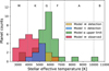 |
Fig. 6 Host star effective temperatures of the planets with metastable helium observations in Fig. 5 separated by the accuracy of the model predictions. In this figure, we adopt a relatively strict factor of two when classifying a model as accurate. So, the red histogram includes the planets for which the model helium EW is more than a factor two higher than the observed EW (i.e., both detections and upper limits toward the bottom-right part of Fig. 5). The blue histogram includes the planets with helium detections that are accurately predicted by our model within a factor two. The green histogram includes the planets where a reported upper limit is above half the model value (i.e., upper limits toward the top-left part of Fig. 5; we consider these consistent as well). The yellow histogram includes the planets with detections that are above two times the model EW (i.e., HAT-P-67 b, HAT-P-32 b, and HD 209458 b). We see that our model tends to overestimate the helium signal particularly for planets around M- and K-type stars. |
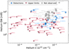 |
Fig. 7 Comparison between the EWs of the metastable helium line and the helium C (a proxy for the expected helium S/N based on the model EW and the J-magnitude; Eq. (B.9)). We include the observed helium planet sample as compiled in Orell-Miquel et al. (2024), as well as potentially good targets that have not yet been observed and have helium C > 3 × 10⁻³ s−1/2 cm−1. For the observed planets, we plot observed EW values, while we plot model EW values for the planets that have not been targeted yet. They are also listed in Table B.1. |
5 Summary
We perform numerical modeling with the sunbather code, to produce synthetic transmission spectra of the upper atmospheres of most transiting exoplanets. The starting point is the NASA Exoplanet Archive, from which we select every transiting planet with reported values for the necessary system parameters. We use a set of stellar SED templates that is mainly comprised of SEDs from the MUSCLES survey. For each planet, the assumed atmospheric mass-loss rate comes from the analytic approximation of Caldiroli et al. (2022), which is based on modeling with the photoevaporation code ATES. The isothermal Parker wind temperature is chosen based on a self-consistency argument. We assume a solar composition upper atmosphere, which may be invalid particularly for sub-Neptune exoplanets. Using all of these ingredients, we calculate high-resolution multi-wavelength (911–11 000 Å) transit spectra of 3898 exoplanets (246 models fail). These spectra are hosted online in the sunset database1.
The large number of transit spectra allows us to study how the strength of spectral lines relates to the bulk planetary parameters. For this, we first filter out the potentially rocky planets. The metastable helium triplet is then found to correlate reasonably strongly with the mass-loss rate. However, the mass-loss rate is certainly not responsible for all of the spread in the helium line strengths, implying that we cannot always equate a nondetection to the absence of atmospheric escape – even for a solar helium abundance. We also find the helium line strength to correlate only moderately with the stellar XUV flux, suggesting that the absence of such a trend in observational studies may, in fact, be not surprising at the current sample sizes. Some other spectral lines such as the calcium infrared triplet and iron NUV multiplet show similar moderately strong correlations with the mass-loss rate. The exception is the C II 1336 Å triplet, which is found to correlate very strongly with the mass-loss rate. The calcium infrared triplet prefers a part of the planetary parameter space (high-gravity planets around early-type stars) that is highly complementary to that of the other lines. Of particular observational interest is the strong correlation between the magnesium doublet and iron multiplet (as they can be targeted in a single HST mode), indicating that their line ratio is an excellent probe of their abundance ratio.
We also compare our synthetic spectra to a near-complete sample of 65 observed metastable helium spectra. Save a few interesting exceptions, our results are generally consistent with the observed census, within the large model uncertainties. This suggests that, to first degree, photoevaporation can explain the present-day landscape of metastable helium observations. Finally, for each of the spectral lines focused on in this work, we define S/N proxies that help to identify the best observational targets.
Acknowledgements
We thank the anonymous referee for their comments and criticisms which have helped to improve the quality of this work. We also thank L. dos Santos, J. Spake, and F. Nail for the helpful conversations. This work has made use of the Snellius Supercomputer operated by SURF. A. Oklopčić gratefully acknowledges support from the Dutch Research Council NWO Veni grant.
Appendix A Additional figures
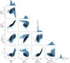 |
Fig. A.1 Correlations between various bulk parameters of the final planet population. The gravitational potential ϕ is calculated directly from the planet mass and radius as reported in the NASA Exoplanet Archive. The XUV flux FXUV comes from the stellar SED template. The mass-loss rate |
![Mathematical equation: $\[\dot{M}\]$](/articles/aa/full_html/2025/06/aa52431-24/aa52431-24-eq19.png)
![Mathematical equation: $\[\bar{\mu}\]$](/articles/aa/full_html/2025/06/aa52431-24/aa52431-24-eq20.png)
 |
Fig. A.2 Correlations between various bulk system parameters and spectral line strengths in the transmission spectrum. The spectral line strengths are expressed as the transit depth at line-center. Specifically, they are the metastable helium line evaluated at 10833.25 Å, the calcium infrared triplet evaluated at 8544.44 Å, the magnesium doublet evaluated at 2796.35 Å, the iron UV2 multiplet evaluated at 2382.76 Å, the carbon triplet evaluated at 1335.68 Å, the oxygen triplet evaluated at 1302.17, and the silicon triplet evaluated at 1264.74 Å. Spearman’s ρ correlation coefficients are quoted in red in each subplot. They are calculated from the quantities as they are labeled on the axes, so in log-log space except for the stellar effective temperature. |
Appendix B Promising targets for various spectral lines
Here, we derive a crude estimate for the expected photon-limited S/N in spectral lines, based on our model-predicted EW, the host star apparent magnitude, and the telescope specifications. We start from the observed stellar magnitude in a photometric band, for example the J-band for metastable helium observations or the V-band for the calcium infrared triplet. The observed specific flux at Earth F is related to the apparent magnitude as
![Mathematical equation: $\[F_X=F_{X, 0} \cdot 10^{-0.4 m_X},\]$](/articles/aa/full_html/2025/06/aa52431-24/aa52431-24-eq21.png) (B.1)
(B.1)
where X denotes a photometric band (J or V), mX is the apparent magnitude in that band, and FX,0 is a reference flux level: FJ,0 = 3.02 × 10⁻¹⁰ erg s−1 cm−2 Å−1 (Campins et al. 1985) and FV,0 = 3.61 × 10⁻⁹ erg s−1 cm−2 Å−1 (Bessell 1979). Since the helium and calcium lines are also present in the stellar spectrum, the stellar flux in those lines will be different from the continuum. To account for this, we can introduce a dimensionless stellar line-depth constant l of order unity, yielding the stellar specific flux in the line as
![Mathematical equation: $\[F_\lambda=F_X \cdot l.\]$](/articles/aa/full_html/2025/06/aa52431-24/aa52431-24-eq22.png) (B.2)
(B.2)
Using a telescope with diameter D, we measure a specific luminosity of
![Mathematical equation: $\[L_\lambda=F_\lambda \cdot \pi(D / 2)^2.\]$](/articles/aa/full_html/2025/06/aa52431-24/aa52431-24-eq23.png) (B.3)
(B.3)
If we observe for a time t and the detector has a throughput of η, we observe a specific energy (i.e., energy per unit wavelength) of
![Mathematical equation: $\[E_\lambda=L_\lambda \cdot \eta t.\]$](/articles/aa/full_html/2025/06/aa52431-24/aa52431-24-eq24.png) (B.4)
(B.4)
Since the energy of a single photon with wavelength λ is Eγ = hc/λ, the detector collects a specific number of stellar photons (i.e., number of photons per unit wavelength)
![Mathematical equation: $\[N_\lambda=\frac{E_\lambda}{E_\gamma}=\frac{E_\lambda \cdot \lambda}{h c}.\]$](/articles/aa/full_html/2025/06/aa52431-24/aa52431-24-eq25.png) (B.5)
(B.5)
Because of the planet’s transit, a portion of these stellar photons are absorbed, forming a spectral line with a certain equivalent width (that we numerically predicted in this work). The total number of absorbed stellar photons is thus
![Mathematical equation: $\[N_{\gamma, p}=N_\lambda \cdot \mathrm{EW}.\]$](/articles/aa/full_html/2025/06/aa52431-24/aa52431-24-eq26.png) (B.6)
(B.6)
This deficit in stellar photons due to the planet’s transit, is measured relative to the total number of stellar photons observed in the line, which is equal to the line-width times Nλ. With high-resolution spectrographs that spectrally resolve the line, the line-width can be approximated by the full-width at half-maximum (FWHM) of the planet’s absorption line. For lower resolution spectrographs that do not spectrally resolve the line (such as the James Webb Space Telescope around the metastable helium line), the line-width is set by the instrument resolution. Here, we proceed by assuming that the spectral line is resolved, so that the total number of stellar photons in the line can be approximated by
![Mathematical equation: $\[N_{\gamma, *}=N_\lambda \cdot \text { FWHM }.\]$](/articles/aa/full_html/2025/06/aa52431-24/aa52431-24-eq27.png) (B.7)
(B.7)
Assuming photon-limited noise (with Nγ,* ≫ 1 so that we can use normal instead of Poissonian errors), the stellar noise becomes ![Mathematical equation: $\[\sqrt{N_{\gamma, *}}\]$](/articles/aa/full_html/2025/06/aa52431-24/aa52431-24-eq28.png) and the S/N becomes
and the S/N becomes
![Mathematical equation: $\[\begin{aligned}\mathrm{S} / \mathrm{N} & =\frac{N_{\lambda, p}}{\sqrt{N_{\gamma, *}}} \\& =\sqrt{\frac{\pi}{4 h c}} \mathrm{EW} \sqrt{\frac{\lambda ~F_{\mathrm{X}, 0}}{\mathrm{FWHM}}} ~10^{-m_X / 5} \sqrt{ln t D^2} \\& =C \sqrt{ln t D^2},\end{aligned}\]$](/articles/aa/full_html/2025/06/aa52431-24/aa52431-24-eq29.png) (B.8)
(B.8)
where we absorbed the terms that do not depend on the observing strategy into the S/N pre-factor
![Mathematical equation: $\[C=\sqrt{\frac{\pi}{4 h c}} \mathrm{EW} \sqrt{\frac{\lambda ~F_{\mathrm{X}, 0}}{\mathrm{FWHM}}} 10^{-m_X / 5}.\]$](/articles/aa/full_html/2025/06/aa52431-24/aa52431-24-eq30.png) (B.9)
(B.9)
We report C for the metastable helium line and calcium infrared triplet in the sunset database. To give an example, for WASP-107 b, the helium C = 0.0436 s−1/2 cm−1 so that if the stellar line depth is l = 0.7, one hour (in-transit) observations with an η = 0.1, D = 10 m telescope such as Keck/NIRSPEC give a predicted S/N of 692. This S/N is probably unrealistically high, because it is based on photon-limited noise. In reality, the S/N of observations will likely be degraded further by other factors, such as instrument noise, stellar variability, and background sky brightness in ground-based observations. If one is interested in obtaining C-values and S/N estimates for unresolved observations (such as those with James Webb Space Telescope), one need only substitute the FWHM by Δλ = λ/R (where R is the instrument’s resolving power) in Eqs. B.8 and B.9. The sunset database reports the FWHM values, so multiplying the C-values by ![Mathematical equation: $\[\sqrt{\mathrm{FWHM} / \Delta \lambda}\]$](/articles/aa/full_html/2025/06/aa52431-24/aa52431-24-eq31.png) will give the desired S/N estimate. In Tables B.1 and B.2, we list the planets with the highest helium and calcium C-values. For this, we only include the 326 exoplanets without the potentially serious warnings listed at the end of Sec. 2.5. WASP-107 b, which was seen to have one of the highest C-values in Fig. 7, is not in the table because it has the warning that its Kϕ value is below the validity bounds of the Caldiroli et al. (2022) formula.
will give the desired S/N estimate. In Tables B.1 and B.2, we list the planets with the highest helium and calcium C-values. For this, we only include the 326 exoplanets without the potentially serious warnings listed at the end of Sec. 2.5. WASP-107 b, which was seen to have one of the highest C-values in Fig. 7, is not in the table because it has the warning that its Kϕ value is below the validity bounds of the Caldiroli et al. (2022) formula.
We do not provide C-values for the other spectral lines studied in this work, because the uncertainties in the stellar background flux are too large. The shortest wavelength photometry that is available for most systems is the B-magnitude, but this is most likely not a good proxy for the stellar flux in the UV lines. We are also not comfortable using the stellar line fluxes from our template SEDs as estimates, because these line fluxes likely vary a lot between different stars of the same spectral type. Therefore, in this work, we trust the overall XUV-flux level of the template stellar SEDs enough to perform the numerical calculations of atmospheric escape, but do not trust the template line fluxes enough to predict the observed S/N in these lines.
To still provide some guidance as to which might be the most promising planets to observe in these UV lines, we defined a more simple transmission-spectroscopy metric (TSM) based only on the predicted EW and the distance to the system:
![Mathematical equation: $\[\text { magnesium/carbon/oxygen } \mathrm{TSM}=\frac{\mathrm{EW}_{\text {line }}}{\lambda_{\text {line }}} \times \frac{7.7 ~\mathrm{pc}}{d},\]$](/articles/aa/full_html/2025/06/aa52431-24/aa52431-24-eq32.png) (B.10)
(B.10)
where EWline and λline are the equivalent width and central wavelength of the line, and d is the distance to the system. We included a factor of 7.7 pc to normalize to the distance of the star Vega, as this star is also used to normalize the other apparent magnitudes. We list the ten planets with the highest TSM in each line in table B.3, B.4, and B.5. The magnesium TSM should also predict the iron and silicon observability well, given their extremely high correlations (Fig. A.2). The metrics defined here are only intended to be used to compare different planets within each metric, not to compare the metrics of different spectral lines.
Best targets for the metastable helium triplet at 10833 Å.
Best targets for the calcium infrared triplet at 8544 Å.
Best targets for the magnesium doublet at 2796 Å, and likely also for the UV2 iron multiplet and the silicon line at 1265 Å, since these line strengths are highly correlated.
Best targets for the carbon triplet at 1336 Å.
Best targets for the oxygen triplet at 1302 Å.
Appendix C Exploration of biases
To perform the simulations in this work, we assumed the values of multiple model parameters. We investigate here how strong the biases and uncertainties are resulting from our choice of two of these parameters specifically. To test this, we first construct a small sample of representative exoplanets. We divide our final population into three equally sized sub-populations of exoplanets with relatively low, medium, and high values of ϕ. We then do the same thing for FXUV, and Teff. We then randomly pick one planet with each possible combination of low, medium, and high values of these three parameters. In other words, we have one planet with low ϕ, low FXUV, and low Teff, another planet with low ϕ, low FXUV, and medium Teff, etc. Our representative sample thus consists of 27 exoplanets that span the parameter space well. We do this based on ϕ, FXUV, and Teff (a proxy for R*, M*, and SED hardness) because we found these parameters to be most important in predicting outflow characteristics such as T0 (see Eq. 2) and EWHe (see Eq. 3).
The first model parameter we investigate is the outer radius of our simulation domain, which we originally fixed at 8Rp. We run the same sample of 27 exoplanets again while using a simulation domain that extends to the stellar radius. For the exoplanets in our sample, R* varies between ~ 5Rp to ~ 61Rp. Table C.1 presents the resulting differences in spectral line strengths. We find that for most lines except for the carbon triplet, the differences are typically within 30% or so. The carbon line can show a larger difference, up to an order of magnitude, which happens for planets that receive low XUV flux. There are also quite a few cases where a spectral line becomes weaker, even though we now use a larger computational domain (i.e., R* is larger than 8Rp). This is due to the fact that we obtained a somewhat different temperature profile, which affects the spectral line formation. Especially if the spectral line forms well below 8Rp (see e.g., Linssen & Oklopčić 2023), the added material beyond 8Rp does not affect the line much, while the different temperature structure does affect the line formation below 8Rp. Therefore, some part of the uncertainty percentages we find here are actually due to sunbather’s temperature convergence algorithm rather than the extent of the computational domain.
Analysis of the bias and uncertainty arising from the chosen extent of the simulation domain.
The second model parameter we investigate is the atmospheric temperature T0, which we originally chose such that it is equal to the maximum of the nonisothermal profile (![Mathematical equation: $\[\hat{T}\]$](/articles/aa/full_html/2025/06/aa52431-24/aa52431-24-eq40.png) , see Sect. 2.3). Here, we quantify the change in our results when we instead use a T0 that is equal to the mean temperature of the nonisothermal profile between 1 and 3 Rp. By definition, this new T0 is lower than the value used in sunset. Table C.2 quantifies the difference in T0, as well as of the spectral line strengths in the transit spectrum. It shows that most of the spectral line depths for most planets are not very strongly affected by the choice of atmospheric temperature (a factor less than a few). However, for each spectral line, there are exceptions for specific types of systems that are more strongly affected (a factor ≲ 10). Furthermore, the calcium infrared triplet is an exception, as many planets react quite sensitively to a change of the chosen temperature. Interesting to note is the fact that we find difference factors > 1 for all spectral lines, meaning that the new models show deeper lines. Given that any reasonably chosen value of T0 should be less than or equal than
, see Sect. 2.3). Here, we quantify the change in our results when we instead use a T0 that is equal to the mean temperature of the nonisothermal profile between 1 and 3 Rp. By definition, this new T0 is lower than the value used in sunset. Table C.2 quantifies the difference in T0, as well as of the spectral line strengths in the transit spectrum. It shows that most of the spectral line depths for most planets are not very strongly affected by the choice of atmospheric temperature (a factor less than a few). However, for each spectral line, there are exceptions for specific types of systems that are more strongly affected (a factor ≲ 10). Furthermore, the calcium infrared triplet is an exception, as many planets react quite sensitively to a change of the chosen temperature. Interesting to note is the fact that we find difference factors > 1 for all spectral lines, meaning that the new models show deeper lines. Given that any reasonably chosen value of T0 should be less than or equal than ![Mathematical equation: $\[\hat{T}\]$](/articles/aa/full_html/2025/06/aa52431-24/aa52431-24-eq41.png) , we arrive at the conclusion that the spectral line strengths in the main work are lower limits with respect to the dependency on T0, and that particularly the calcium line could be a lot stronger than predicted in the main work.
, we arrive at the conclusion that the spectral line strengths in the main work are lower limits with respect to the dependency on T0, and that particularly the calcium line could be a lot stronger than predicted in the main work.
Analysis of the bias and uncertainty arising from the chosen atmospheric temperature.
References
- Allart, R., Bourrier, V., Lovis, C., et al. 2018, Science, 362, 1384 [Google Scholar]
- Allart, R., Lemée-Joliecoeur, P.-B., Jaziri, A. Y., et al. 2023, A&A, 677, A164 [NASA ADS] [CrossRef] [EDP Sciences] [Google Scholar]
- Alonso-Floriano, F. J., Snellen, I. A. G., Czesla, S., et al. 2019, A&A, 629, A110 [NASA ADS] [CrossRef] [EDP Sciences] [Google Scholar]
- Ballabio, G., & Owen, J. E. 2025, MNRAS, 537, 1305 [Google Scholar]
- Ballester, G. E., & Ben-Jaffel, L. 2015, ApJ, 804, 116 [Google Scholar]
- Behr, P. R., France, K., Brown, A., et al. 2023, AJ, 166, 35 [NASA ADS] [CrossRef] [Google Scholar]
- Bello-Arufe, A., Knutson, H. A., Mendonça, J. M., et al. 2023, AJ, 166, 69 [NASA ADS] [CrossRef] [Google Scholar]
- Ben-Jaffel, L., & Ballester, G. E. 2013, A&A, 553, A52 [NASA ADS] [CrossRef] [EDP Sciences] [Google Scholar]
- Benneke, B., Roy, P.-A., Coulombe, L.-P., et al. 2024, arXiv e-prints [arXiv:2403.03325] [Google Scholar]
- Bennett, K. A., Redfield, S., Oklopčić, A., et al. 2023, AJ, 165, 264 [NASA ADS] [CrossRef] [Google Scholar]
- Bessell, M. S. 1979, PASP, 91, 589 [Google Scholar]
- Bourrier, V., & Lecavelier des Etangs, A. 2013, A&A, 557, A124 [NASA ADS] [CrossRef] [EDP Sciences] [Google Scholar]
- Bourrier, V., Lecavelier Des Etangs, A., Ehrenreich, D., et al. 2018, A&A, 620, A147 [NASA ADS] [CrossRef] [EDP Sciences] [Google Scholar]
- Burn, R., Mordasini, C., Mishra, L., et al. 2024, Nat. Astron., 8, 463 [Google Scholar]
- Caldiroli, A., Haardt, F., Gallo, E., et al. 2021, A&A, 655, A30 [NASA ADS] [CrossRef] [EDP Sciences] [Google Scholar]
- Caldiroli, A., Haardt, F., Gallo, E., et al. 2022, A&A, 663, A122 [NASA ADS] [CrossRef] [EDP Sciences] [Google Scholar]
- Campins, H., Rieke, G. H., Lebofsky, M. J., & Observatory, S. 1985, AJ, 90, 896 [Google Scholar]
- Carolan, S., Vidotto, A. A., Hazra, G., Villarreal D’Angelo, C., & Kubyshkina, D. 2021, MNRAS, 508, 6001 [NASA ADS] [CrossRef] [Google Scholar]
- Chatzikos, M., Bianchi, S., Camilloni, F., et al. 2023, Rev. Mex. Astron. Astrofis., 59, 327 [Google Scholar]
- Chen, J., & Kipping, D. 2017, ApJ, 834, 17 [Google Scholar]
- Czesla, S., Lampón, M., Sanz-Forcada, J., et al. 2022, A&A, 657, A6 [NASA ADS] [CrossRef] [EDP Sciences] [Google Scholar]
- Dos Santos, L. A., Ehrenreich, D., Bourrier, V., et al. 2019, A&A, 629, A47 [NASA ADS] [CrossRef] [EDP Sciences] [Google Scholar]
- dos Santos, L. A., Vidotto, A. A., Vissapragada, S., et al. 2022, A&A, 659, A62 [NASA ADS] [CrossRef] [EDP Sciences] [Google Scholar]
- Ehrenreich, D., Bourrier, V., Wheatley, P. J., et al. 2015, Nature, 522, 459 [Google Scholar]
- Erkaev, N. V., Kulikov, Y. N., Lammer, H., et al. 2007, A&A, 472, 329 [NASA ADS] [CrossRef] [EDP Sciences] [Google Scholar]
- Farret Jentink, C., Pepe, F., Lovis, C., et al. 2024a, in Ground-based and Airborne Instrumentation for Astronomy X, 291 [CrossRef] [Google Scholar]
- Farret Jentink, C., Bourrier, V., Lovis, C., et al. 2024b, MNRAS, 527, 4467 [Google Scholar]
- Ferland, G. J., Chatzikos, M., Guzman, F., et al. 2017, Rev. Mex. Astron. Astrofis., 53, 385 [Google Scholar]
- Fossati, L., Koskinen, T., Lothringer, J. D., et al. 2018, ApJ, 868, L30 [CrossRef] [Google Scholar]
- Fossati, L., Guilluy, G., Shaikhislamov, I. F., et al. 2022, A&A, 658, A136 [NASA ADS] [CrossRef] [EDP Sciences] [Google Scholar]
- Fossati, L., Pillitteri, I., Shaikhislamov, I. F., et al. 2023, A&A, 673, A37 [NASA ADS] [CrossRef] [EDP Sciences] [Google Scholar]
- France, K., Loyd, R. O. P., Youngblood, A., et al. 2016, ApJ, 820, 89 [NASA ADS] [CrossRef] [Google Scholar]
- Fulton, B. J., Petigura, E. A., Howard, A. W., et al. 2017, AJ, 154, 109 [Google Scholar]
- García Muñoz, A., Fossati, L., Youngblood, A., et al. 2021, ApJ, 907, L36 [Google Scholar]
- Gialluca, M. T., Barnes, R., Meadows, V. S., et al. 2024, Planet. Sci. J., 5, 137 [Google Scholar]
- Greene, T. P., Bell, T. J., Ducrot, E., et al. 2023, Nature, 618, 39 [NASA ADS] [CrossRef] [Google Scholar]
- Gronoff, G., Arras, P., Baraka, S., et al. 2020, JGR (Space Phys.), 125, e2019JA027639 [CrossRef] [Google Scholar]
- Guilluy, G., D’Arpa, M. C., Bonomo, A. S., et al. 2024, A&A, 686, A83 [NASA ADS] [CrossRef] [EDP Sciences] [Google Scholar]
- Gully-Santiago, M., Morley, C. V., Luna, J., et al. 2024, AJ, 167, 142 [NASA ADS] [CrossRef] [Google Scholar]
- Gupta, S., Basak, A., & Nandy, D. 2023, ApJ, 953, 70 [Google Scholar]
- Ho, C. S. K., & Van Eylen, V. 2023, MNRAS, 519, 4056 [NASA ADS] [CrossRef] [Google Scholar]
- Hori, Y., & Ogihara, M. 2020, ApJ, 889, 77 [NASA ADS] [CrossRef] [Google Scholar]
- Kasper, D., Bean, J. L., Oklopčić, A., et al. 2020, AJ, 160, 258 [Google Scholar]
- Kempton, E. M.-R., Zhang, M., Bean, J. L., et al. 2023, Nature, 620, 67 [NASA ADS] [CrossRef] [Google Scholar]
- Kirk, J., Dos Santos, L. A., López-Morales, M., et al. 2022, AJ, 164, 24 [NASA ADS] [CrossRef] [Google Scholar]
- Koskinen, T. T., Aylward, A. D., & Miller, S. 2007, Nature, 450, 845 [CrossRef] [Google Scholar]
- Krishnamurthy, V., & Cowan, N. B. 2024, AJ, 168, 30 [NASA ADS] [CrossRef] [Google Scholar]
- Kubyshkina, D., Fossati, L., & Erkaev, N. V. 2024, A&A, 684, A26 [NASA ADS] [CrossRef] [EDP Sciences] [Google Scholar]
- Kulow, J. R., France, K., Linsky, J., & Parke Loyd, R. O. 2014, ApJ, 786, 132 [NASA ADS] [CrossRef] [Google Scholar]
- Kurokawa, H., & Nakamoto, T. 2014, ApJ, 783, 54 [NASA ADS] [CrossRef] [Google Scholar]
- Lamers, H. J. G. L. M., & Cassinelli, J. P. 1999, Introduction to Stellar Winds (Cambridge University Press) [Google Scholar]
- Lampón, M., López-Puertas, M., Lara, L. M., et al. 2020, A&A, 636, A13 [NASA ADS] [CrossRef] [EDP Sciences] [Google Scholar]
- Lavie, B., Ehrenreich, D., Bourrier, V., et al. 2017, A&A, 605, L7 [NASA ADS] [CrossRef] [EDP Sciences] [Google Scholar]
- Lecavelier des Etangs, A., Ehrenreich, D., Vidal-Madjar, A., et al. 2010, A&A, 514, A72 [NASA ADS] [CrossRef] [EDP Sciences] [Google Scholar]
- Linsky, J. L., Yang, H., France, K., et al. 2010, ApJ, 717, 1291 [Google Scholar]
- Linssen, D. C., & Oklopčić, A. 2023, A&A, 675, A193 [NASA ADS] [CrossRef] [EDP Sciences] [Google Scholar]
- Linssen, D., Shih, J., MacLeod, M., & Oklopčić, A. 2024, A&A, 688, A43 [NASA ADS] [CrossRef] [EDP Sciences] [Google Scholar]
- Linssen, D. C., Oklopčić, A., & MacLeod, M. 2022, A&A, 667, A54 [NASA ADS] [CrossRef] [EDP Sciences] [Google Scholar]
- Loyd, R. O. P., France, K., Youngblood, A., et al. 2016, ApJ, 824, 102 [NASA ADS] [CrossRef] [Google Scholar]
- Loyd, R. O. P., Koskinen, T. T., France, K., Schneider, C., & Redfield, S. 2017, ApJ, 834, L17 [Google Scholar]
- MacLeod, M., & Oklopčić, A. 2022, ApJ, 926, 226 [NASA ADS] [CrossRef] [Google Scholar]
- Nail, F., Oklopčić, A., & MacLeod, M. 2024, A&A, 684, A20 [NASA ADS] [CrossRef] [EDP Sciences] [Google Scholar]
- Nortmann, L., Pallé, E., Salz, M., et al. 2018, Science, 362, 1388 [Google Scholar]
- Oklopčić, A. 2019, ApJ, 881, 133 [Google Scholar]
- Oklopčić, A., & Hirata, C. M. 2018, ApJ, 855, L11 [Google Scholar]
- Orell-Miquel, J., Murgas, F., Pallé, E., et al. 2022, A&A, 659, A55 [NASA ADS] [CrossRef] [EDP Sciences] [Google Scholar]
- Orell-Miquel, J., Murgas, F., Pallé, E., et al. 2024, A&A, 689, A179 [NASA ADS] [CrossRef] [EDP Sciences] [Google Scholar]
- Otegi, J. F., Bouchy, F., & Helled, R. 2020, A&A, 634, A43 [NASA ADS] [CrossRef] [EDP Sciences] [Google Scholar]
- Owen, J. E., & Lai, D. 2018, MNRAS, 479, 5012 [Google Scholar]
- Paragas, K., Vissapragada, S., Knutson, H. A., et al. 2021, ApJ, 909, L10 [NASA ADS] [CrossRef] [Google Scholar]
- Parker, E. N. 1958, ApJ, 128, 664 [Google Scholar]
- Poppenhaeger, K. 2022, MNRAS, 512, 1751 [CrossRef] [Google Scholar]
- Rottman, G. 2005, Sol. Phys., 230, 7 [NASA ADS] [CrossRef] [Google Scholar]
- Rumenskikh, M. S., Khodachenko, M. L., Shaikhislamov, I. F., et al. 2023, MNRAS, 526, 4120 [NASA ADS] [Google Scholar]
- Saidel, M., Vissapragada, S., Spake, J., et al. 2025, AJ, 169, 104 [Google Scholar]
- Salz, M., Czesla, S., Schneider, P. C., & Schmitt, J. H. M. M. 2016, A&A, 586, A75 [NASA ADS] [CrossRef] [EDP Sciences] [Google Scholar]
- Schlawin, E., Agol, E., Walkowicz, L. M., Covey, K., & Lloyd, J. P. 2010, ApJ, 722, L75 [NASA ADS] [CrossRef] [Google Scholar]
- Sing, D. K., Lavvas, P., Ballester, G. E., et al. 2019, AJ, 158, 91 [Google Scholar]
- Spake, J. J., Sing, D. K., Evans, T. M., et al. 2018, Nature, 557, 68 [Google Scholar]
- Stassun, K. G., Oelkers, R. J., Paegert, M., et al. 2019, AJ, 158, 138 [Google Scholar]
- Szabó, G. M., & Kiss, L. L. 2011, ApJ, 727, L44 [Google Scholar]
- Venturini, J., Guilera, O. M., Haldemann, J., Ronco, M. P., & Mordasini, C. 2020, A&A, 643, L1 [NASA ADS] [CrossRef] [EDP Sciences] [Google Scholar]
- Vidal-Madjar, A., des Etangs, A. L., Désert, J.-M., et al. 2003, Nature, 422, 143 [Google Scholar]
- Vidal-Madjar, A., Désert, J.-M., Etangs, A. L. d., et al. 2004, ApJ, 604, L69 [NASA ADS] [CrossRef] [Google Scholar]
- Vidotto, A. A., & Bourrier, V. 2017, MNRAS, 470, 4026 [NASA ADS] [CrossRef] [Google Scholar]
- Vissapragada, S., Knutson, H. A., Jovanovic, N., et al. 2020, AJ, 159, 278 [Google Scholar]
- Vissapragada, S., Knutson, H. A., Greklek-McKeon, M., et al. 2022, AJ, 164, 234 [NASA ADS] [CrossRef] [Google Scholar]
- Wang, L., & Dai, F. 2021, ApJ, 914, 98 [NASA ADS] [CrossRef] [Google Scholar]
- Wilson, D. J., Froning, C. S., Duvvuri, G. M., et al. 2021, ApJ, 911, 18 [NASA ADS] [CrossRef] [Google Scholar]
- Wogan, N. F., Batalha, N. E., Zahnle, K. J., et al. 2024, ApJ, 963, L7 [NASA ADS] [CrossRef] [Google Scholar]
- Woods, T. N., Eparvier, F. G., Bailey, S. M., et al. 2005, JGR (Space Phys.), 110 [Google Scholar]
- Yan, F., Casasayas-Barris, N., Molaverdikhani, K., et al. 2019, A&A, 632, A69 [NASA ADS] [CrossRef] [EDP Sciences] [Google Scholar]
- Yelle, R. V. 2004, Icarus, 170, 167 [NASA ADS] [CrossRef] [Google Scholar]
- Youngblood, A., France, K., Loyd, R. O. P., et al. 2016, ApJ, 824, 101 [Google Scholar]
- Zhang, M., Knutson, H. A., Wang, L., et al. 2021, AJ, 161, 181 [NASA ADS] [CrossRef] [Google Scholar]
- Zhang, M., Knutson, H. A., Wang, L., Dai, F., & Barragán, O. 2022, AJ, 163, 67 [NASA ADS] [CrossRef] [Google Scholar]
- Zhang, M., Dai, F., Bean, J. L., Knutson, H. A., & Rescigno, F. 2023a, ApJ, 953, L25 [NASA ADS] [CrossRef] [Google Scholar]
- Zhang, M., Knutson, H. A., Dai, F., et al. 2023b, AJ, 165, 62 [NASA ADS] [CrossRef] [Google Scholar]
- Zhang, Z., Morley, C. V., Gully-Santiago, M., et al. 2023c, Sci. Adv., 9, eadf8736 [NASA ADS] [CrossRef] [Google Scholar]
- Zhang, M., Bean, J. L., Wilson, D., et al. 2025, AJ, 169, 204 [Google Scholar]
- Zieba, S., Kreidberg, L., Ducrot, E., et al. 2023, Nature, 620, 746 [NASA ADS] [CrossRef] [Google Scholar]
The sunset database: https://zenodo.org/records/13785440
This table is only present in their arXiv pre-print version: 2404.16732.
All Tables
Best targets for the magnesium doublet at 2796 Å, and likely also for the UV2 iron multiplet and the silicon line at 1265 Å, since these line strengths are highly correlated.
Analysis of the bias and uncertainty arising from the chosen extent of the simulation domain.
Analysis of the bias and uncertainty arising from the chosen atmospheric temperature.
All Figures
|
Fig. 1 Top: stellar spectral energy distribution templates used in this work. The A0 and A7 spectra are based on the work of Fossati et al. (2018), the solar spectrum is from the TIMED and SORCE missions (Woods et al. 2005; Rottman 2005), and the rest of the spectra are from the MUSCLES survey (France et al. 2016; Youngblood et al. 2016; Loyd et al. 2016; Wilson et al. 2021; Behr et al. 2023). Bottom: integrated XUV flux (λ < 911 Å) of each SED as a function of the effective temperature of the star (scatter points; see also Table 1). Small black points indicate SEDs in the MUSCLES database that we do not use. The grey histogram (read from the right y-axis) shows the host star effective temperatures of the initial planet population. Planets are assigned the SED template of the closest stellar spectral type. If the spectral type is not reported, the SED template of the star with the closest effective temperature is assigned. |
| In the text | |
|
Fig. 2 Mass-loss rates of the initial planet population calculated from the analytical approximation of Caldiroli et al. (2022, Appendix A). The mass-loss rate is parametrized as a function of Rp, Mp, a, M*, and FXUV, based on the output of the first-principle 1D photoevaporation code ATES (Caldiroli et al. 2021). The shaded lower region indicates planets with radii <2.5RE, which are potentially rocky. We do produce spectra for these planets that we include in sunset, but do not include them when analyzing our final planet population in Sect. 3. |
| In the text | |
|
Fig. 3 Example of the publicly available1 output data products for the planet TOI-3235 b (simulated with sunbather; Linssen et al. 2024). Left column: upper atmospheric structure. Right column: zoom-in on various parts of the transmission spectrum. The full spectrum spans 911 Å to 11 000 Å at a spectral resolution of R ~ 400 000. It includes spectral lines from the 30 lightest elements (up until zinc). |
| In the text | |
|
Fig. 4 Fit to the isothermal Parker wind temperature as a function of the planetary gravitational potential and received XUV flux. The final planet population (scatter points) is fitted with a power law (grey plane). The functional form is given by Eq. (2). The systematic residuals reveals that this functional form is not optimal, and particularly does not fully capture the dependence on the gravity. |
| In the text | |
|
Fig. 5 Comparison between the observed and modeled EW of the metastable helium line for the near-complete planet sample as compiled in Orell-Miquel et al. (2024). The dotted line is x = y (i.e., complete agreement). The model uncertainties are very large. Rough estimates of the uncertainty due to the XUV flux (based on the scaling in Eq. (3)), the helium abundance (based on additional simulations of TOI-2018 b), and the metallicity (based on simulations of Linssen et al. 2024 of a generic hot Neptune planet) are indicated. An additional significant source of uncertainty is the shape of the stellar SED (specifically the ratio between EUV and NUV flux). Compared to the model uncertainties, observational uncertainties are very small (typically inside the size of the scatter marker) and therefore not shown. |
| In the text | |
|
Fig. 6 Host star effective temperatures of the planets with metastable helium observations in Fig. 5 separated by the accuracy of the model predictions. In this figure, we adopt a relatively strict factor of two when classifying a model as accurate. So, the red histogram includes the planets for which the model helium EW is more than a factor two higher than the observed EW (i.e., both detections and upper limits toward the bottom-right part of Fig. 5). The blue histogram includes the planets with helium detections that are accurately predicted by our model within a factor two. The green histogram includes the planets where a reported upper limit is above half the model value (i.e., upper limits toward the top-left part of Fig. 5; we consider these consistent as well). The yellow histogram includes the planets with detections that are above two times the model EW (i.e., HAT-P-67 b, HAT-P-32 b, and HD 209458 b). We see that our model tends to overestimate the helium signal particularly for planets around M- and K-type stars. |
| In the text | |
|
Fig. 7 Comparison between the EWs of the metastable helium line and the helium C (a proxy for the expected helium S/N based on the model EW and the J-magnitude; Eq. (B.9)). We include the observed helium planet sample as compiled in Orell-Miquel et al. (2024), as well as potentially good targets that have not yet been observed and have helium C > 3 × 10⁻³ s−1/2 cm−1. For the observed planets, we plot observed EW values, while we plot model EW values for the planets that have not been targeted yet. They are also listed in Table B.1. |
| In the text | |
|
Fig. A.1 Correlations between various bulk parameters of the final planet population. The gravitational potential ϕ is calculated directly from the planet mass and radius as reported in the NASA Exoplanet Archive. The XUV flux FXUV comes from the stellar SED template. The mass-loss rate |
| In the text | |
|
Fig. A.2 Correlations between various bulk system parameters and spectral line strengths in the transmission spectrum. The spectral line strengths are expressed as the transit depth at line-center. Specifically, they are the metastable helium line evaluated at 10833.25 Å, the calcium infrared triplet evaluated at 8544.44 Å, the magnesium doublet evaluated at 2796.35 Å, the iron UV2 multiplet evaluated at 2382.76 Å, the carbon triplet evaluated at 1335.68 Å, the oxygen triplet evaluated at 1302.17, and the silicon triplet evaluated at 1264.74 Å. Spearman’s ρ correlation coefficients are quoted in red in each subplot. They are calculated from the quantities as they are labeled on the axes, so in log-log space except for the stellar effective temperature. |
| In the text | |
Current usage metrics show cumulative count of Article Views (full-text article views including HTML views, PDF and ePub downloads, according to the available data) and Abstracts Views on Vision4Press platform.
Data correspond to usage on the plateform after 2015. The current usage metrics is available 48-96 hours after online publication and is updated daily on week days.
Initial download of the metrics may take a while.