| Issue |
A&A
Volume 693, January 2025
|
|
|---|---|---|
| Article Number | A222 | |
| Number of page(s) | 11 | |
| Section | Interstellar and circumstellar matter | |
| DOI | https://doi.org/10.1051/0004-6361/202452270 | |
| Published online | 20 January 2025 | |
Molecular chemistry induced by a J-shock toward supernova remnant W51C
1
School of Astronomy & Space Science, Nanjing University,
163 Xianlin Avenue,
Nanjing
210023,
China
2
Laboratoire d’Astrophysique de Bordeaux, Univ. Bordeaux, CNRS, B18N,
allée Geoffroy Saint-Hilaire,
33615
Pessac,
France
3
Key Laboratory of Modern Astronomy and Astrophysics, Nanjing University, Ministry of Education,
Nanjing
210023,
China
★ Corresponding author; This email address is being protected from spambots. You need JavaScript enabled to view it.
Received:
17
September
2024
Accepted:
9
December
2024
Abstract
Context. Shock waves from supernova remnants (SNRs) strongly affect the physical and chemical properties of molecular clouds (MCs). Shocks propagating into magnetized MCs can be classified into jump or J-shocks and continuous or C-shocks. The molecular chemistry in the re-formed molecular gas behind J-shocks is still only poorly understood. It is expected to provide a comprehensive view of the chemical feedback of SNRs and the chemical effects of J-shocks.
Aims. We conducted a W-band (71.4–89.7 GHz) observation toward a re-formed molecular clump behind a J-shock induced by SNR W51C with the Yebes 40 m radio telescope to study the molecular chemistry in the re-formed molecular gas.
Methods. Assuming local thermodynamic equilibrium (LTE), we estimated the column densities of HCO+, HCN, C2H and o-c-C3H2, and derived their abundance ratio maps with CO. The gas density was constrained by a non-LTE analysis of the HCO+ J = 1–0 line. The abundance ratios were compared with the values in typical quiescent MCs and shocked MCs, and they were also compared with the results of chemical simulations with the Paris-Durham shock code to verify and investigate the chemical effects of J-shocks.
Results. We obtained the following abundance ratios: N(HCO+)/N(CO) ~ (1.0–4.0) × 10−4, N(HCN)/N(CO) ~ (1.8–5.3) × 10−4, N(C2H)/N(CO) ~ (1.6–5.0) × 10−3, and N(o-c-C3H2)/N(CO) ~ (1.2–7.9) × 10−4. The non-LTE analysis suggests that the gas density is nH2 ≳ 104 cm−3. We find that the N(C2H)/N(CO) and N(o-c-C3H2)/N(CO) are higher than typical values in quiescent MCs and shocked MCs by 1–2 orders of magnitude, which can be qualitatively attributed to the abundant C+ and C in the earliest phase of molecular gas re-formation. The Paris-Durham shock code can reproduce, although not perfectly, the observed abundance ratios, especially the enhanced N(C2H)/N(CO) and N(c-C3H2)/N(CO), with J-shocks propagating into both nonirradiated and irradiated molecular gas with a preshock density of nH = 2 × 103 cm−3.
Key words: shock waves / ISM: abundances / ISM: clouds / ISM: molecules / ISM: supernova remnants
© The Authors 2025
 Open Access article, published by EDP Sciences, under the terms of the Creative Commons Attribution License (https://creativecommons.org/licenses/by/4.0), which permits unrestricted use, distribution, and reproduction in any medium, provided the original work is properly cited.
This article is published in open access under the Subscribe to Open model. This email address is being protected from spambots. You need JavaScript enabled to view it. to support open access publication.
1 Introduction
Supernova remnants (SNRs) exert a strong influence on the physical and chemical properties of the molecular clouds (MCs) with which they interact (e.g., van Dishoeck et al. 1993). Among all the effects driven by SNRs, the shock waves play a crucial rule. A shock can heat, compress, and accelerate the molecular gas (Draine & McKee 1993), which alters the physical properties of the MC and regulates the molecular chemistry through various processes (e.g., Burkhardt et al. 2019).
The shocks that propagate into magnetized MCs can roughly be classified into two types: jump or J-shocks, and continuous or C-shocks (Draine & McKee 1993). J-shocks are often fast and weakly magnetized. The deceleration and heating of the entire shock is almost entirely due to the viscous stresses arising in a thin transition layer called the viscous subshock. A jump in the physical parameters (density, temperature, etc.) is expected in the shock profile. In contrast, C-shocks are often slow and strongly magnetized. The momentum transfer and heating are completed by the magnetic precursor that precedes the viscous subshock when the magnetic field is strong enough to cause the magnetosonic speed ![Mathematical equation: $\[(B / \sqrt{4 \pi \rho_{i}})\]$](/articles/aa/full_html/2025/01/aa52270-24/aa52270-24-eq1.png) to be higher than the shock velocity. Therefore, the physical parameters change continuously without a jump between the upstream and downstream.
to be higher than the shock velocity. Therefore, the physical parameters change continuously without a jump between the upstream and downstream.
Molecular chemistry induced by C-shocks has been extensively studied in SNRs (e.g., van Dishoeck et al. 1993; Lazendic et al. 2010; Zhou et al. 2022; Tu et al. 2024a) and in other astro-physical environments such as molecular outflows of protostars (e.g., Bachiller et al. 2001; Mendoza et al. 2018; Codella et al. 2020). Since C-shocks are nondissociative, most molecules can survive, and C-shocks can also release the depleted molecular species back into the gas phase and make them detectable (e.g., SiO, Gusdorf et al. 2008). However, investigations of molecular chemistry induced by J-shock are hampered by the fact that a J-shock can result in a much higher temperature than a C-shock, and most molecules will be dissociated (e.g., Kristensen et al. 2023). Therefore, observational studies of J-shocks often turn to emission lines of atoms (e.g., Rho et al. 2001; Lee et al. 2019) or infrared transitions of a limited variety of molecules: CO, H2, and H2O (e.g., Shinn et al. 2012; Rho et al. 2015). However, simulations have found that molecules can re-form in the cooling gas behind a fast and dissociative J-shock (Hollenbach & McKee 1989; Neufeld & Dalgarno 1989; Cuppen et al. 2010; Hollenbach et al. 2013), and observations also found this reformed molecular gas in SNRs W51C (Koo & Moon 1997b) and IC443 (Wang & Scoville 1992). In the prototypical protostellar outflow L1157, molecular gas that re-formed behind the J-shock was identified by CO observations (Lefloch et al. 2012; Benedettini et al. 2012), and re-formed CS was discovered (Gómez-Ruiz et al. 2015). However, the abundance of CS deviates little from other C-shocked components. It is still unclear whether a J-shock can induce a different chemistry compared with a C-shock and quiescent gas conditions.
SNR W51C (G49.2–0.7) is a middle-aged SNR that interacts with MCs, as shown by 1720 MHz OH masers (Green et al. 1997), the broadened molecular line (Koo & Moon 1997b; Brogan et al. 2013), SiO emission (Dumas et al. 2014), and so on. Cold CO gas that re-formed behind a J-shock was found by Koo & Moon (1997b) based on three observational facts. First, the local-standard-of-rest (LSR) velocity of the CO gas (≳80 km s−1) is higher than the tangent point LSR velocity (≈60 km s−1) in this direction (l ≈ 49°). The CO gas is therefore likely accelerated by the shock to high LSR velocity. Second, the line-of-sight velocity separation between the preshock and postshock CO gas is large (≈20–50 km s−1), while for a C-shock, the postshock gas should be at velocities closer to that of the preshock gas since the acceleration of the shocked gas is continuous. Third, the estimated excitation temperature of the CO emission is low (~10 K), and it is expected to be higher for C-shocked gas. Fourth, the postshock CO gas is spatially and spectrally coincident with high-velocity HI gas, which was proposed to be subject to a fast shock with a velocity of ~100 km s−1 (Koo & Moon 1997a).
We present a new molecular observation toward clump 2 of W51C that was found and named by Koo & Moon (1997b) to study the detailed molecular chemistry induced by a J-shock. In Sect. 2 we describe the details of our observation and the data reduction. The observational results are presented in Sect. 3. In Sect. 4 we calculate the molecular column densities and abundance ratios, constrain the gas density, discuss the chemistry of carbon-chain species, and present the results of our chemical simulation. Our conclusions are summarized in Sect. 5.
2 Observations
2.1 Yebes 40 m observation
We conducted a new mapping observation toward clump 2 (which was identified and named by Koo & Moon 1997b) of SNR W51C with the Yebes 40 m radio telescope (PI: Tian-Yu Tu, project code: 24A003) in W band, covering the spectral range of 71.4–89.7 GHz. Position-switching mode was adopted throughout the observation, with the reference point at αJ2000 = 19h23m05s.8, δJ2000 = +14°10′56″. The mapping was made toward a 82″.5 × 82″.5 region centered at αJ2000 = 19h22m45s.69, δJ2000 = +14°11′58″.9 with a pixel size of 7″.5 × 7″.5 (see Fig. 1 for the position and size of the mapped region). The sensitivity measured in the main-beam temperature Tmb at the raw spectral resolution (38 kHz) was 0.05–0.09 K. The data were reduced with the GILDAS/CLASS package1. For better comparison, all of the reduced data cubes were smoothed to a common beam size of 27″.6.
2.2 Other archival data
We obtained some archival data to support our analysis. The 12CO J = 3–2 data were retrieved from the 12CO (3–2) High-Resolution Survey (COHRS) project (Park et al. 2023) performed by the James Clarke Maxwell Telescope (JCMT). The angular resolution was 16.6″, and the sensitivity measured in ![Mathematical equation: $\[T_{\mathrm{A}}^{*}\]$](/articles/aa/full_html/2025/01/aa52270-24/aa52270-24-eq2.png) was ~1 K at a velocity channel width of 0.635 km s−1. The antenna temperature was converted into Tmb with a main-beam efficiency of 0.61.
was ~1 K at a velocity channel width of 0.635 km s−1. The antenna temperature was converted into Tmb with a main-beam efficiency of 0.61.
We also obtained the 12CO J = 1–0 data observed by the Nobeyama 45 m telescope and the [C I] (3P1−3P0) data observed by the Atacama Submillimeter Telescope Experiment (ASTE) 10 m telescope from Yamagishi et al. (2023). The details of the observation can be found therein. All of these supplementary data cubes were smoothed to a beam size of 27″.6.
The 1.4 GHz radio continuum map of W51C was obtained from the VLA Galactic Plane Survey (VGPS, Stil et al. 2006). All the processed data were further analyzed with the Python packages Astropy (Astropy Collaboration 2018, 2022) and Spectral-cube2. The data cubes of the CO isotopes were reprojected with the reproject3 package. We visualized the data with the Python package Matplotlib4.
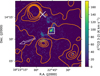 |
Fig. 1 Integrated-intensity map of the JCMT 12CO J = 3–2 line in the velocity range +80− +110 km s−1, which is the velocity range of the re-formed CO gas proposed by Koo & Moon (1997b), overlaid with orange contours of the VGPS 1.4 GHz radio continuum (the levels are 50–250 K in steps of 50 K). The two white crosses show the 1720 MHz OH masers discovered by Green et al. (1997). The white arrow points to the geometric center of W51C recorded in the Green SNR catalog (Green 2019). The white box shows the molecular clump toward which we conducted the Yebes 40 m observation. |
3 Results
In total, we detected transitions from 24 molecular species, five of which (HCO+, HCN, C2H, o-c-C3H2, and H2CO) show broadened emission-line profiles in the velocity range +80−+110 km s−1, which is the LSR velocity range of the re-formed CO gas (Koo & Moon 1997b), while others are only detected around ~ +61 km s−1 which corresponds to the ambient MCs. The spectra of the five molecular transitions averaged in the entire mapped region, together with the 12CO (hereafter CO if not specified) J = 1–0 and 3–2 lines, are shown in Fig. 2. The averaged spectra of other detected molecular species are shown in the appendix. The HCO+ and HCN lines exhibit the highest signal-to-noise ratio. Considering that the HCN line may be affected by the hyperfine structures, we used the HCO+ line to analyze the velocity structure in the mapped region.
We divided the entire HCO+ spectrum into six components (see the colored rectangles in Fig. 2) based on visual inspections of their spatial distributions. The integrated intensity maps of the six components are shown in Fig. 3. Component (a) is bright toward the southwest of the mapped region and is not spatially coincident with the radio continuum. Component (b) is mainly located in the north and is spatially coincident with the 870 μm far-infrared continuum dust emission detected by the APEX Telescope Large Area Survey of the GALaxy (ATLASGAL, Urquhart et al. 2018). The emission peak of HCO+ in this component is also consistent with the ATLASGAL clump G49.111–0.322. Components (c) and (d) are contiguous in the spectrum: (c) is an emission peak, and (d) exhibits a line wing structure (see Fig. 2). However, component (c) is located toward the east of (d) and is spatially coincident with a bulge in the radio continuum. Both components could be preshock gas of W51C or C-shocked gas. Components (e) and (f) are separated from the other velocity components and have been proposed to be the molecular gas that re-formed behind a fast J-shock. However, these two components show a slightly different spatial distribution. The majority of the emission in component (e) is toward the center of the mapped region, while this component also contains a weak emission feature toward the west. For component (f), the emission toward the west vanishes, while the emission peak moves east compared with component (e). The spatial distribution of component (f) is similar to (c) and is also coincident with a bulge in the radio continuum.
Although the re-formed gas can be divided into two velocity components, it is hard to perform spectral decomposition because the shocked gas does not necessarily exhibit a Gaussian line profile and the signal-to-noise ratio of the other transitions is limited. In the following analysis, we regard the two components as one. We also note that none of components (a) to (d) can undoubtedly be identified as the preshock gas. A pixel-by-pixel decomposition of all the observed spectra around 61 km s−1 is also almost impossible. Therefore, we cannot directly estimate the properties of the preshock gas from our observation.
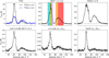 |
Fig. 2 Spectra of the molecular transitions with emission detected in the velocity range +80− +110 km s−1 averaged across the entire mapped region. The velocity integration intervals for the six velocity components are shown by colored rectangles in the spectrum of HCO+. |
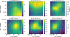 |
Fig. 3 HCO+ integrated intensity map of the six velocity components marked by colored rectangles in Fig. 2. The solid orange contours show the VGPS 1.4 GHz radio continuum at 104–112 K levels in steps of 2 K from left (east) to right (west), and the dashed orange contours show the ATLASGAL 870 μm continuum (in steps of 0.3, 0.6, and 0.9 Jy beam−1). The red cross in panel (b) shows the position of ATLASGAL clump G49.111–0.322. |
4 Discussion
4.1 Estimating the molecular column densities and abundance ratios
Considering that we lack data of multiple (≥3) transitions of one molecular species, we assumed local thermodynamic equilibrium (LTE) in our estimation of the molecular column densities. We assumed that all the transitions in the velocity range +80−+110 km s−1 were optically thin because their line widths are large, which in turn suggests large velocity gradients. The excitation temperature (Tex) of the CO lines can be estimated by fitting the relation (Goldsmith & Langer 1999)
![Mathematical equation: $\[\log \frac{N_{u}}{g_{u}}=~\log~ N-~\log~ Z-\frac{E_{u}}{k T_{\mathrm{ex}}},\]$](/articles/aa/full_html/2025/01/aa52270-24/aa52270-24-eq3.png) (1)
(1)
where Nu is the column density of the molecules in the upper energy level, gu is the statistical weight of the upper energy level, N is the total column density, Z is the partition function, and Eu is the energy of the upper level. In the optical thin limit, Nu can be written as Nu = (8πkν2W)/(hc3Aul), where W is the integrated intensity, and Aul is the Einstein A coefficient of the transition. After we obtained Tex, we estimated the column density via (Mangum & Shirley 2015)
![Mathematical equation: $\[N=\frac{3 k}{8 \pi^{3} \nu} \frac{Z ~\exp~ \left(E_{\mathrm{u}} / k T_{\mathrm{ex}}\right)}{S \mu^{2}} \frac{J_{\nu}\left(T_{\mathrm{ex}}\right)}{J_{\nu}\left(T_{\mathrm{ex}}\right)-J_{\nu}\left(T_{\mathrm{bg}}\right)} W,\]$](/articles/aa/full_html/2025/01/aa52270-24/aa52270-24-eq4.png) (2)
(2)
where S is the line strength, μ is the dipole moment, Tbg = 2.73 K is the background temperature, and Jν(T) is defined by Jν(T) = (hν/k)/(exp (hν/kT) − 1). The molecular constants (Eu and Sμ2) were retrieved from Splatalogue5. The obtained Tex(CO) and N(CO) maps are shown in Fig. 4. Generally, the Tex(CO) is within the range 11.5–23 K, and the N(CO) is within 1–9 × 1016 cm−2 throughout the clump. The peaks of both values are higher than those obtained by Koo & Moon (1997a), which are Tex = 11 K and N(CO) = 4 × 1016 cm−2, because the beam size of our data (27″.6) is smaller than that of their data (55″, in which the beam dilution effect is stronger because the angular size of the source is smaller than the beam size).
To estimate the column densities of other molecular species, we made two assumptions on their Tex: (1) We assumed that Tex of the other species is equal to Tex(CO), and (2) we fixed Tex = 5 K (van der Tak et al. 2007) throughout the target region for other species because they trace gas that is denser than CO (Shirley 2015). We did not estimate the column density of H2CO because the signal-to-noise ratio of its transition is low. The abundance ratio maps of N(HCO+)/N(CO), N(HCN)/N(CO), N(C2H)/N(CO), and N(o-c-C3H2)/N(CO) based on the two assumptions are separately shown in Fig. 5. Here we cannont obtain the abundances of HCO+, HCN, C2H and o-c-C3H2 because the abundance of CO is not necessarily ~10−4 at these low column densities (e.g., Burgh et al. 2007).
Fig. 5 shows that the difference between the abundance ratios estimated for the two assumed cases of Tex is within a factor of 2 for HCO+, HCN and C2H, and a factor of 3 for o-c-C3H2. The obtained ranges of the abundance ratios, including the values obtained with the two assumptions, are 1.0–4.0 × 10⁻⁴, 1.8–5.3 × 10⁻⁴, 1.6–5.0 × 10⁻³, and 1.2–7.9 × 10⁻⁴ for N(HCO+)/N(CO), N(HCN)/N(CO), N(C2H)/N(CO), and N(o-c-C3H2)/N(CO), respectively. The abundance ratios are all highest toward the eastern edge of the molecular clump and decrease toward the west, which is roughly consistent with the direction of the SNR blast wave.
We also estimated an upper limit of the N(C0)/N(CO) considering that no broadened [C I] emission (see Sect. 2.2) is detected. The upper limit of N(C0) can be estimated with (Izumi et al. 2021)
![Mathematical equation: $\[\begin{aligned}& N\left(\mathrm{C}^0\right)=4.67 \times 10^{16} \\& \quad \times \frac{1+3 ~\exp \left(-23.6 / T_{\mathrm{ex}}\right)+5 ~\exp \left(-62.5 / T_{\mathrm{ex}}\right)}{1-~\exp \left(-23.6 / T_{\mathrm{ex}}\right)} \int \tau_{[\mathrm{C~I}]} d v,\end{aligned}\]$](/articles/aa/full_html/2025/01/aa52270-24/aa52270-24-eq5.png) (3)
(3)
where the optical depth of the [C I] line is
![Mathematical equation: $\[\tau_{[\mathrm{C~I}]}=-~\ln \left[1-\frac{T_{\mathrm{mb}}}{J_{\nu}(T_{\mathrm{ex}})-J_{\nu}(T_{\mathrm{bg}})}\right].\]$](/articles/aa/full_html/2025/01/aa52270-24/aa52270-24-eq6.png) (4)
(4)
We assumed that the nondetected [C I] line profile follows a Gaussian with a full width at half maximum (FWHM) of 15 km s−1. We smoothed the original data to a beam of 27″.6 (see Sect. 2.2) and a velocity channel width of 3 km s−1. The 3σ upper limit of the Tmb is 0.5 K. We varied the Tex from 12 K to 22 K to determine the maximum upper limit of N(C0). Finally, we found an upper limit for N(C0)/N(CO) of ≲2.
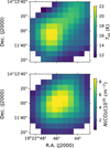 |
Fig. 4 Excitation temperature (upper panel) and column density (lower panel) maps of CO. |
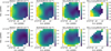 |
Fig. 5 Maps of the abundance ratios N(HCO+)/N(CO), N(HCN)/N(CO), N(C2H)/N(CO), and N(o-c-C3H2)/N(CO) (from left to right) based on the assumptions Tex = Tex(CO) (upper row) and Tex = 5 K (lower row). |
4.2 Constraint on the gas density
Although we were unable to conduct a non-LTE analysis to fit the physical parameters of the molecular clump, we still constrained its gas density. The peak integrated intensity of the HCO+ J = 1–0 line is ≈ 12 K km s−1 (which was inferred by combining Figs. 3e and f), and the peak N(HCO+) in the LTE analysis is ~2 × 1013 cm−2 (which was inferred by combining Figs. 4 and 5). We note that although the LTE analysis is indeed not precise, we considered N(HCO+) for two cases of Tex of 5 K and ~20 K as the lower and upper ends of the Tex range separately. Therefore, the estimated peak can be regarded as a strict upper limit of the real N(HCO+). To constrain the gas density, we ran a set of physical parameters with the non-LTE radiative transfer code RADEX (van der Tak et al. 2007), varying the gas density nH2 and gas temperature T with fixed N(HCO+) = 2 × 1013 cm−2 and an FWHM of 15 km s−1. Similar method was used by Shirley (2015) to estimate the effective excitation density of dense gas tracers. We plot the predicted integrated intensity and the gas density at given values of T in Fig. 6. We find that the gas density must be ~104 cm−3 at least to reproduce the observed peak intensity of the HCO+ J = 1–0 line. Although a higher gas temperature also enhances the integrated intensity at nH2 ≲ 105 cm−3, this effect is not significant at T ≳ 50 K.
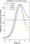 |
Fig. 6 Predicted integrated intensity of HCO+ J = 1–0 line as a function of nH2. The lines with different colors show the models with different gas temperatures. The dotted black line in the right panel shows an integrated intensity of 12 K km s−1. |
4.3 Unusual N(C2H)/N(CO) and N(o-c-C3H2)/N(CO) abundance ratios
We recall that the estimated abundance ratio is ~10−3 for N(C2H)/N(CO) and ~10−4 for N(o-c-C3H2)/N(CO). In dense quiescent MCs, these ratios are typically ~10−4−10−5 and ~10−5−10−6, respectively (e.g., Agúndez & Wakelam 2013; Kim et al. 2020). Therefore, the obtained N(C2H)/N(CO) and N(o-c-C3H2)/N(CO) ratios are higher than the typical values in dense MCs by 1–2 orders of magnitude.
Broadened emission line induced by SNR-MC interaction of C2H was only found in SNRs IC443 (van Dishoeck et al. 1993), W28 (Mazumdar et al. 2022), and 3C391 (Tu et al. 2024b), while broadened c-C3H2 line was only found in SNR 3C391 (Tu et al. 2024b). The N(C2H)/N(CO) toward IC443 clump G, which is one of the prototypical molecular clumps interacting with SNRs, is ~10−4 (van Dishoeck et al. 1993), which is similar to the value in typical quiescent MCs. In other environments of interstellar shocks, C2H and c-C3H2 are also discussed rarely. For example, these two species are regarded as tracers of ambient gas (e.g., Shimajiri et al. 2015) or cavity walls exposed to UV radiation (e.g., Tychoniec et al. 2021) in protostellar outflows. In the molecular cloud core L1521, which is a source of shocked carbon-chain chemistry with an enhanced abundance of some carbon-chain species, the abundance ratio N(c-C3H2)/N(CO) is ~10−5 (Sato et al. 1994; Liu et al. 2021). We note that the ortho-to-para ratio of c-C3H2 is 3 in thermal equilibrium and is often observed to be within the range of 1–3 (Park et al. 2006). Therefore, the column density of o-c-C3H2 is expected to be similar to that of c-C3H2, and the observed N(c-C3H2)/N(CO) value toward L1251 is lower than the value we obtained in W51C by an order of magnitude. A high N(C2H)/N(CO) ratio similar to our case was found in the circumnuclear disk of the Seyfert galaxy NGC 1068 (Viti et al. 2014; Nakajima et al. 2023), but it was proposed to be the result of a complex interaction with a shock and UV or X-ray radiation (García-Burillo et al. 2017).
Our observed abundance ratios are roughly consistent with the values in diffuse or translucent molecular gas: Liszt & Lucas (1998) for CO, Lucas & Liszt (1996) for HCO+, Liszt & Lucas (2001) for HCN, and Lucas & Liszt (2000) for C2H and c-C3H2; see also Table 3 of Liszt et al. (2006) for a compilation. We also refer to Kim et al. (2023) for a later observation of all the species except CO. However, the gas density of the target clump (≳104 cm−3) is higher than the typical values of diffuse and translucent clouds (Snow & McCall 2006). Therefore, the dominating physical and chemical processes are expected to be different.
Carbon-chain species, including C2H and c-C3H2, are regarded as early-type species (Sakai & Yamamoto 2013; Taniguchi et al. 2024). The formation of carbon-chain species strongly relies on C+ and C0 in the gas phase (see Fig. 1 of Sakai & Yamamoto 2013 and Fig. 1 of Taniguchi et al. 2024), which are transformed into CO as the cloud evolves from diffuse gas into molecular cloud core. For instance, the formation routes of C2H include but are not limited to (Taniguchi et al. 2024)
![Mathematical equation: $\[\begin{array}{l}(a) \mathrm{C}^{+} \xrightarrow{\mathrm{H}_{2}} \mathrm{CH}_{2}^{+} \xrightarrow{\mathrm{H}_{2}} \mathrm{CH}_{3}^{+} \xrightarrow{\mathrm{e}^{-}} \mathrm{CH}_{2} \xrightarrow{\mathrm{C}^{+}} \mathrm{C}_{2} \mathrm{H}\\(b) \mathrm{C}^{+} \xrightarrow{\mathrm{H}_{2}} \mathrm{CH}_{2}^{+} \xrightarrow{\mathrm{H}_{2}} \mathrm{CH}_{3}^{+} \xrightarrow{\mathrm{C}} \mathrm{C}_{2} \mathrm{H}_{2}^{+} \xrightarrow{\mathrm{e}^{-}} \mathrm{C}_{2} \mathrm{H}\\(c) \mathrm{C}^{+} \xrightarrow{\mathrm{H}_{2}} \mathrm{CH}_{2}^{+} \xrightarrow{\mathrm{e}^{-}} \mathrm{CH} \xrightarrow{\mathrm{C}^{+}} \mathrm{C}_{2}^{+} \xrightarrow{\mathrm{H}_{2}} \mathrm{C}_{2} \mathrm{H}^{+} \xrightarrow{\mathrm{H}_{2}} \mathrm{C}_{2} \mathrm{H}_{2}^{+} \xrightarrow{\mathrm{e}^{-}} \mathrm{C}_{2} \mathrm{H}.\end{array}\]$](/articles/aa/full_html/2025/01/aa52270-24/aa52270-24-eq7.png) (5)
(5)
Therefore, carbon chains are formed efficiently in the earliest phase of MC formation and are depleted or destructed in evolved MCs. This was verified by many chemical simulations (e.g., Suzuki et al. 1992; Taniguchi et al. 2019). Since the target clump is molecular gas that re-formed behind a dissociative J-shock, it is thought to be in the earliest phase of the MC evolution with abundant C+ and C0 in the gas phase. Therefore, enhanced abundances of carbon-chain species, and in turn, their abundance ratios to CO, are possible. The simulation of Neufeld & Dalgarno (1989) also predicted a plateau of the C2H abundance X(C2H) soon after the J-shock. However, this simulation only considered a fast J-shock in dense preshock gas >104 cm−3, which is higher than the preshock density in our case, and it did not predict a significantly enhanced N(C2H)/N(CO) abundance ratio either.
4.4 Chemical simulation of molecular re-formation behind a J-shock
To further investigate whether the enhanced N(C2H)/N(CO) and N(o-c-C3H2)/N(CO) abundance ratios are due to the chemistry induced by the J-shock, we used the Paris-Durham shock code (Flower et al. 1985; Flower & Pineau des Forêts 2003, 2015; Godard et al. 2019) to simulate the molecular re-formation behind a J-shock. The code is a public numerical tool for computing the coupled dynamical, thermal, and chemical evolution of the interstellar medium subject to a plane-parallel shock wave. The computation consisted of two steps. In step 1, the code simulated the evolution of a quiescent cloud and evolved it into a steady state. In step 2, the code used the outputs of step 1 as the preshock conditions (including the physical and chemical parameters) and allowed a shock wave to propagate into the preshock cloud.
We simulated both irradiated and nonirradiated shocks. In the irradiated case, we assumed that a cloud with a visual extinction of AV = 2 (at the interface between the translucent and dense MC (Snow & McCall 2006)) was irradiated by the interstellar radiation field with G0 = 1.6 in Habing unit6 (Parravano et al. 2003; Wolfire et al. 2022). The magnetic field in the simulation was controlled by a parameter ![Mathematical equation: $\[\beta=B(\mu \mathrm{G}) / \sqrt{n_{\mathrm{H}}(\mathrm{cm}^{-3})}\]$](/articles/aa/full_html/2025/01/aa52270-24/aa52270-24-eq8.png) . We adopted β = 1, which is close to the magnetic field in interstellar clouds (Crutcher et al. 2010). The cosmic-ray ionization rate per H2 was fixed to be 1.3 × 10⁻¹⁷ s−1 in step 1, which is the typical value in MCs (Caselli et al. 1998), and it was enhanced to 5 × 10⁻¹⁶ s−1 in step 2, which is roughly consistent with previous observations and simulations (Ceccarelli et al. 2011; Shingledecker et al. 2016; Yamagishi et al. 2023). The propagation time of the shock was limited to t < 3 × 10⁴ yr, which is consistent with previous constraints on the age of W51C (Koo et al. 1995; Park et al. 2013). We varied the preshock H nucleus density nH to be 2 × 10², 2 × 10³, and 2 × 104 cm−3, and the shock velocity Vs to 25, 30, 40, 50, and 60 km s−1. At lower Vs, the shock becomes a C-shock. We found that a preshock density nH = 2 × 103 cm−3 can reproduce the observed abundance ratio better, and the target clump has a density nH2 ≳ 104 cm−3. Therefore, we limited our discussion to nH = 2 × 103 cm−3.
. We adopted β = 1, which is close to the magnetic field in interstellar clouds (Crutcher et al. 2010). The cosmic-ray ionization rate per H2 was fixed to be 1.3 × 10⁻¹⁷ s−1 in step 1, which is the typical value in MCs (Caselli et al. 1998), and it was enhanced to 5 × 10⁻¹⁶ s−1 in step 2, which is roughly consistent with previous observations and simulations (Ceccarelli et al. 2011; Shingledecker et al. 2016; Yamagishi et al. 2023). The propagation time of the shock was limited to t < 3 × 10⁴ yr, which is consistent with previous constraints on the age of W51C (Koo et al. 1995; Park et al. 2013). We varied the preshock H nucleus density nH to be 2 × 10², 2 × 10³, and 2 × 104 cm−3, and the shock velocity Vs to 25, 30, 40, 50, and 60 km s−1. At lower Vs, the shock becomes a C-shock. We found that a preshock density nH = 2 × 103 cm−3 can reproduce the observed abundance ratio better, and the target clump has a density nH2 ≳ 104 cm−3. Therefore, we limited our discussion to nH = 2 × 103 cm−3.
Figure 7 shows the abundance ratios predicted by the nonirradiated (upper row) and irradiated (lower row) shock models. For the nonirradiated shock model, all of the four abundance ratios except N(C2H)/N(CO) can be well reproduced, while the difference between the peak values of the modeled N(C2H)/N(CO) and observed range is within an order of magnitude. Therefore, we conclude that the observed abundance ratio can essentially be reproduced by the J-shock chemistry. We note that N(C2H)/N(CO) and N(c-C3H2)/N(CO) reach their peak values at ~3 × 10³ yr and then decrease quickly. This is consistent with the scenario according to which the carbon-chain species are early-type species and are destructed during the evolution of the MC (Sakai & Yamamoto 2013; Taniguchi et al. 2024). Specifically, C2H is mainly formed via
![Mathematical equation: $\[\mathrm{CH}^{+} \xrightarrow{\mathrm{H}_{2}} \mathrm{CH}_{2}^{+} \xrightarrow{\mathrm{H}_{2}} \mathrm{CH}_{3}^{+} \xrightarrow{\mathrm{C}} \mathrm{C}_{2} \mathrm{H}_{2}^{+} \xrightarrow{\mathrm{e}^{-}} \mathrm{C}_{2} \mathrm{H},\]$](/articles/aa/full_html/2025/01/aa52270-24/aa52270-24-eq9.png) (6)
(6)
at t ≲ 3 kyr, where the CH+ can be formed through either C+ + H2 or C + ![Mathematical equation: $\[\mathrm{H}_{3}^{+}\]$](/articles/aa/full_html/2025/01/aa52270-24/aa52270-24-eq10.png) . This pathway is similar to route (b) mentioned in reactions 5. Atomic C, which is key to the formation of
. This pathway is similar to route (b) mentioned in reactions 5. Atomic C, which is key to the formation of ![Mathematical equation: $\[\mathrm{C}_{2} \mathrm{H}_{2}^{+}\]$](/articles/aa/full_html/2025/01/aa52270-24/aa52270-24-eq11.png) , is formed in the J-shock through the dissociation of CO and CH. At t ≳ 3 kyr, C2H is mainly destructed by atomic O to form CO. The formation of c-C3H2 is much more complicated and ends with c-C3
, is formed in the J-shock through the dissociation of CO and CH. At t ≳ 3 kyr, C2H is mainly destructed by atomic O to form CO. The formation of c-C3H2 is much more complicated and ends with c-C3![Mathematical equation: $\[\mathrm{H}_{3}^{+}\]$](/articles/aa/full_html/2025/01/aa52270-24/aa52270-24-eq12.png) + e− → c-C3H2 + H, where the c-C3
+ e− → c-C3H2 + H, where the c-C3![Mathematical equation: $\[\mathrm{H}_{3}^{+}\]$](/articles/aa/full_html/2025/01/aa52270-24/aa52270-24-eq13.png) molecule can be formed via c-C3H+/c-C3
molecule can be formed via c-C3H+/c-C3![Mathematical equation: $\[\mathrm{H}_{2}^{+}\]$](/articles/aa/full_html/2025/01/aa52270-24/aa52270-24-eq14.png) + H2.
+ H2.
For the irradiated shock model, N(HCO+)/N(CO) and N(C2H)/N(CO) can be well reproduced, while N(c-C3H2)/N(CO) is within an order of magnitude away from the observed range. However, the N(HCN)/N(CO) is strongly overestimated by the irradiated model. Therefore, although this model can roughly reproduce the observed abundance ratios, its performance is worse than that of the nonirradiated shock model. The formation pathway of C2H in the irradiated shock model is slightly different from that in the nonirradiated shock model,
![Mathematical equation: $\[\mathrm{C}^{+} \xrightarrow{\mathrm{H}_{2}} \mathrm{CH}^{+} \xrightarrow{\mathrm{C}} \mathrm{C}_{2}^{+} \xrightarrow{\mathrm{H}_{2}} \mathrm{C}_{2} \mathrm{H}^{+} \xrightarrow{\mathrm{H}_{2}} \mathrm{C}_{2} \mathrm{H}_{2}^{+} \xrightarrow{\mathrm{e}^{-}} \mathrm{C}_{2} \mathrm{H},\]$](/articles/aa/full_html/2025/01/aa52270-24/aa52270-24-eq15.png) (7)
(7)
because the abundance of C and C+ is higher due to the external UV field.
We note that although both models can reproduce the observed abundance ratios to some extent, the simulation is not exempt from problems. We recall that there are some other constraints on the physical properties of the target molecular clump. Koo & Moon (1997b) found that the abundance ratio N(CO)/N(H I) is <4 × 10⁻⁵, which is the expected value if CO has totally been re-formed while HI has yet to form H2. To explain this effect, they proposed that the hydrogen nuclei are mainly in atomic form instead of molecular, according to the N(H I) versus N(CO) scatter plot (see their Fig. 5). However, as plotted in the left panel of Fig. 8, a significant fraction of H has recombined to H2 even before 2 × 10³ yr, regardless of the shock velocity in the nonirradiated shock models. Therefore, the nonirradiated shock models can hardly reproduce the trends proposed by Koo & Moon (1997b). On the other hand, for the irradiated models, the N(CO)/N(H I) < 4 × 10⁻⁵ can be naturally explained by the fact that neither CO nor H2 has been remarkably re-formed (see the middle panel of Fig. 8). In Sect. 4.1 we obtained an upper limit for the N(C0)/N(CO) abundance ratio ≲2, however. The irradiated shock models may have significantly overestimated the N(C0)/N(CO) abundance ratio, however, because of photodissociation of incident UV radiation. The reason might be that the target clump lies in a weaker UV field than we assumed. An alternative explanation is the uncertainty in the treatment of UV radiative transfer in the shock model, as shown in Godard et al. (2019).
In summary, our simulation can essentially reproduce the observed abundance ratios despite some defects, especially the enhanced N(C2H)/N(CO) and N(c-C3H2)/N(CO). This suggests that these abundance ratios can be explained by the chemistry induced by the J-shock. However, we also note that the chemical simulation shows problems, such as the lacking consideration of the three-dimensional structure of the MC and the incomplete chemical network. In addition, we only investigated some specific cases with simple assumptions on the properties such as the UV field, the magnetic field, and and the cosmic-ray ionization rate, instead of exploring the full parameter space. Further improvement on the chemical network, especially the grain-surface chemistry, which strongly affects the initial condition of the shock and plays an important role in carbon-chain chemistry (Sakai & Yamamoto 2013), and the treatment of UV radiative transfer, may help the shock model to better reproduce the observation, but this is beyond the scope of this paper, however.
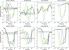 |
Fig. 7 Abundance ratios of N(HCO+)/N(CO), N(HCN)/N(CO), N(C2H)/N(CO) and N(c-C3H2)/N(CO) (from left to right) predicted by the Paris-Durham shock code as a function of time with a preshock density of nH = 2 × 103 cm−3. The upper row shows the results of a nonirradiated shock, and the lower row shows the results of a shock irradiated by an interstellar radiation field (G0 = 1.6) with a visual extinction of AV = 2. The lines with different colors show the results of different shock velocities, as shown in the labels of the upper right panel. The gray shaded regions delineate the range obtained from our observation. |
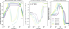 |
Fig. 8 Auxiliary results of the nonirradiated (left panel) and irradiated (middle and right panel) shock models with a preshock density of nH = 2 × 103 cm−3. The lines with different colors show the results of different shock velocities, as shown in the labels of the right panel. Left panel: evolution of the abundances (denoted by X) of H (solid lines) and H2 (dotted lines) relative to the total H nucleus in the nonirradiated models. Middle panel: evolution of the abundances of H (solid lines, multiplied by a factor of 4 × 10⁻⁵) and CO (dotted lines) relative to the total H nucleus in the irradiated models. Right panel: evolution of the abundance ratio N(C0)/N(CO) in the irradiated models. |
5 Conclusions
We presented new observation toward W51C clump 2 in 71.4–89.7 GHz with the Yebes 40 m radio telescope to study the molecular chemistry induced by a J-shock. Five molecular species (HCO+, HCN, C2H, o-c-C3H2, and H2CO) exhibit broadened emission line profiles in +80−+110 km s−1 which is the velocity range of the re-formed molecular gas behind a J-shock. We found that the spectrum of HCO+ J = 1–0 can be divided into six velocity components, in which the re-formed gas can be divided into two components with different spatial distributions. To facilitate the analysis, we regarded the two re-formed gas components as one.
With the CO J = 1–0 and 3–2 data, we estimated the excitation temperature and column density of CO based on the LTE assumption, and obtained the abundance ratios of HCO+, HCN, C2H, o-c-C3H2 to CO, which are N(HCO+)/N(CO) ~ (1.0–4.0) × 10−4, N(HCN)/N(CO) ~ (1.8–5.3) × 10−4, N(C2H)/N(CO) ~ (1.6–5.0) × 10−3, and N(o-c-C3H2)/N(CO) ~ (1.2–7.9) × 10−4. We also obtained an upper limit for the N(C0)/N(CO) abundance ratio of ≲2. We found that the N(C2H)/N(CO) and o-c-C3H2 ratios are higher than the typical values in dense MCs and the value in SNR IC443 clump G. This enhancement can be qualitatively attributed to the chemistry in the earliest phase of MC formation, when abundant C+ and C in the gas phase boost the formation of carbon-chain species.
To further investigate whether the enhanced N(C2H)/N(CO) and N(c-C3H2)/N(CO) are due to J-shock chemistry, we conducted a chemical simulation with the Paris-Durham shock code. We found that the nonirradiated and irradiated shock models with a preshock density of nH = 2 × 103 cm−3 can both basically reproduce the observed abundance ratios, despite some defects. This suggests that the abundance ratios can indeed be attributed to the chemistry induced by a J-shock. However, the nonirradiated models overestimate the re-formation of H2, while the irradiated models overestimate the N(C0)/N(CO) abundance ratio. Improvements of the shock code may help to reproduce the observation.
Acknowledgements
The authors thank Alba Vidal García who carried out the observations and the first inspection of the data quality, other staff of the Yebes observatory who supported the observation and data transmission, Mitsuyoshi Yamagishi who provided the data cubes of 12CO and [C I], and Benjamin Godard who offered helps on the use of the Paris-Durham shock code. V.W. acknowledges the CNRS program “Physique et Chimie du Milieu Interstellaire” (PCMI) co-funded by the Centre National d’Etudes Spatiales (CNES). Y.C. acknowledges the support from NSFC grants Nos. 12173018 and 12121003. P.Z. acknowledges the support from NSFC grant No. 12273010. This article is based on observations carried out with the Yebes 40 m telescope (project code: 24A003). The 40 m radio telescope at Yebes Observatory is operated by the Spanish Geographic Institute (IGN; Ministerio de Transportes y Movilidad Sostenible). This work has made use of the Paris-Durham public shock code V1.1, distributed by the CNRS-INSU National Service “ISM Platform” at the Paris Observatory Data Center (http://ism.obspm.fr).
Appendix A Spectra of all other detected transitions
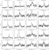 |
Fig. A.1 Spectra of all detected molecular transitions averaged in the entire field of view except those which have been shown in Fig. 2. |
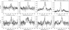 |
Fig. A.2 Continued. The HCS+ J = 2–1 line is at ≈ +29 km s−1 in the upper right panel of which the rest frequency is set to be the frequency of the o-c-C3H2 line. |
References
- Agúndez, M., & Wakelam, V. 2013, ChRv, 113, 8710 [Google Scholar]
- Astropy Collaboration (Price-Whelan, A. M., et al.) 2018, ApJ, 156, 123 [CrossRef] [Google Scholar]
- Astropy Collaboration (Price-Whelan, A. M., et al.) 2022, ApJ, 935, 167 [NASA ADS] [CrossRef] [Google Scholar]
- Bachiller, R., Pérez Gutiérrez, M., Kumar, M. S. N., & Tafalla, M. 2001, A&A, 372, 899 [NASA ADS] [CrossRef] [EDP Sciences] [Google Scholar]
- Benedettini, M., Busquet, G., Lefloch, B., et al. 2012, A&A, 539, L3 [NASA ADS] [CrossRef] [EDP Sciences] [Google Scholar]
- Brogan, C. L., Goss, W. M., Hunter, T. R., et al. 2013, ApJ, 771, 91 [NASA ADS] [CrossRef] [Google Scholar]
- Burgh, E. B., France, K., & McCandliss, S. R. 2007, ApJ, 658, 446 [NASA ADS] [CrossRef] [Google Scholar]
- Burkhardt, A. M., Shingledecker, C. N., Le Gal, R., et al. 2019, ApJ, 881, 32 [Google Scholar]
- Caselli, P., Walmsley, C. M., Terzieva, R., & Herbst, E. 1998, ApJ, 499, 234 [Google Scholar]
- Ceccarelli, C., Hily-Blant, P., Montmerle, T., et al. 2011, ApJ, 740, L4 [NASA ADS] [CrossRef] [Google Scholar]
- Codella, C., Ceccarelli, C., Bianchi, E., et al. 2020, A&A, 635, A17 [NASA ADS] [CrossRef] [EDP Sciences] [Google Scholar]
- Crutcher, R. M., Wandelt, B., Heiles, C., Falgarone, E., & Troland, T. H. 2010, ApJ, 725, 466 [NASA ADS] [CrossRef] [Google Scholar]
- Cuppen, H. M., Kristensen, L. E., & Gavardi, E. 2010, MNRAS, 406, L11 [NASA ADS] [Google Scholar]
- Draine, B. T., & McKee, C. F. 1993, ARA&A, 31, 373 [NASA ADS] [CrossRef] [Google Scholar]
- Dumas, G., Vaupré, S., Ceccarelli, C., et al. 2014, ApJ, 786, L24 [NASA ADS] [CrossRef] [Google Scholar]
- Flower, D. R., & Pineau des Forêts, G. 2003, MNRAS, 343, 390 [Google Scholar]
- Flower, D. R., & Pineau des Forêts, G. 2015, A&A, 578, A63 [NASA ADS] [CrossRef] [EDP Sciences] [Google Scholar]
- Flower, D. R., Pineau des Forêts, G., & Hartquist, T. W. 1985, MNRAS, 216, 775 [NASA ADS] [CrossRef] [Google Scholar]
- García-Burillo, S., Viti, S., Combes, F., et al. 2017, A&A, 608, A56 [Google Scholar]
- Godard, B., Pineau des Forêts, G., Lesaffre, P., et al. 2019, A&A, 622, A100 [NASA ADS] [CrossRef] [EDP Sciences] [Google Scholar]
- Goldsmith, P. F., & Langer, W. D. 1999, ApJ, 517, 209 [Google Scholar]
- Gómez-Ruiz, A. I., Codella, C., Lefloch, B., et al. 2015, MNRAS, 446, 3346 [Google Scholar]
- Green, D. A. 2019, JApA, 40, 36 [NASA ADS] [Google Scholar]
- Green, A. J., Frail, D. A., Goss, W. M., & Otrupcek, R. 1997, ApJ, 114, 2058 [CrossRef] [Google Scholar]
- Gusdorf, A., Cabrit, S., Flower, D. R., & Pineau Des Forêts, G. 2008, A&A, 482, 809 [NASA ADS] [CrossRef] [EDP Sciences] [Google Scholar]
- Hollenbach, D., & McKee, C. F. 1989, ApJ, 342, 306 [Google Scholar]
- Hollenbach, D., Elitzur, M., & McKee, C. F. 2013, ApJ, 773, 70 [NASA ADS] [CrossRef] [Google Scholar]
- Izumi, N., Fukui, Y., Tachihara, K., et al. 2021, PASJ, 73, 174 [NASA ADS] [CrossRef] [Google Scholar]
- Kim, W. J., Wyrowski, F., Urquhart, J. S., et al. 2020, A&A, 644, A160 [NASA ADS] [CrossRef] [EDP Sciences] [Google Scholar]
- Kim, W. J., Schilke, P., Neufeld, D. A., et al. 2023, A&A, 670, A111 [NASA ADS] [CrossRef] [EDP Sciences] [Google Scholar]
- Koo, B.-C., & Moon, D.-S. 1997a, ApJ, 475, 194 [NASA ADS] [CrossRef] [Google Scholar]
- Koo, B.-C., & Moon, D.-S. 1997b, ApJ, 485, 263 [NASA ADS] [CrossRef] [Google Scholar]
- Koo, B.-C., Kim, K.-T., & Seward, F. D. 1995, ApJ, 447, 211 [NASA ADS] [CrossRef] [Google Scholar]
- Kristensen, L. E., Godard, B., Guillard, P., Gusdorf, A., & Pineau des Forêts, G. 2023, A&A, 675, A86 [NASA ADS] [CrossRef] [EDP Sciences] [Google Scholar]
- Lazendic, J. S., Wardle, M., Whiteoak, J. B., Burton, M. G., & Green, A. J. 2010, MNRAS, 409, 371 [CrossRef] [Google Scholar]
- Lee, Y.-H., Koo, B.-C., Lee, J.-J., Burton, M. G., & Ryder, S. 2019, ApJ, 157, 123 [CrossRef] [Google Scholar]
- Lefloch, B., Cabrit, S., Busquet, G., et al. 2012, ApJ, 757, L25 [Google Scholar]
- Liszt, H. S., & Lucas, R. 1998, A&A, 339, 56 [NASA ADS] [Google Scholar]
- Liszt, H., & Lucas, R. 2001, A&A, 370, 576 [NASA ADS] [CrossRef] [EDP Sciences] [Google Scholar]
- Liszt, H. S., Lucas, R., & Pety, J. 2006, A&A, 448, 253 [NASA ADS] [CrossRef] [EDP Sciences] [Google Scholar]
- Liu, X. C., Wu, Y., Zhang, C., et al. 2021, ApJ, 912, 148 [NASA ADS] [CrossRef] [Google Scholar]
- Lucas, R., & Liszt, H. 1996, A&A, 307, 237 [NASA ADS] [Google Scholar]
- Lucas, R., & Liszt, H. S. 2000, A&A, 358, 1069 [NASA ADS] [Google Scholar]
- Mangum, J. G., & Shirley, Y. L. 2015, PASA, 127, 266 [CrossRef] [Google Scholar]
- Mazumdar, P., Tram, L. N., Wyrowski, F., Menten, K. M., & Tang, X. 2022, A&A, 668, A180 [NASA ADS] [CrossRef] [EDP Sciences] [Google Scholar]
- Mendoza, E., Lefloch, B., Ceccarelli, C., et al. 2018, MNRAS, 475, 5501 [NASA ADS] [CrossRef] [Google Scholar]
- Nakajima, T., Takano, S., Tosaki, T., et al. 2023, ApJ, 955, 27 [NASA ADS] [CrossRef] [Google Scholar]
- Neufeld, D. A., & Dalgarno, A. 1989, ApJ, 340, 869 [Google Scholar]
- Park, I. H., Wakelam, V., & Herbst, E. 2006, A&A, 449, 631 [NASA ADS] [CrossRef] [EDP Sciences] [Google Scholar]
- Park, G., Koo, B. C., Gibson, S. J., et al. 2013, ApJ, 777, 14 [NASA ADS] [CrossRef] [Google Scholar]
- Park, G., Currie, M. J., Thomas, H. S., et al. 2023, ApJS, 264, 16 [NASA ADS] [CrossRef] [Google Scholar]
- Parravano, A., Hollenbach, D. J., & McKee, C. F. 2003, ApJ, 584, 797 [Google Scholar]
- Rho, J., Jarrett, T. H., Cutri, R. M., & Reach, W. T. 2001, ApJ, 547, 885 [CrossRef] [Google Scholar]
- Rho, J., Hewitt, J. W., Boogert, A., Kaufman, M., & Gusdorf, A. 2015, ApJ, 812, 44 [NASA ADS] [CrossRef] [Google Scholar]
- Sakai, N., & Yamamoto, S. 2013, ChRv, 113, 8981 [NASA ADS] [Google Scholar]
- Sato, F., Mizuno, A., Nagahama, T., et al. 1994, ApJ, 435, 279 [NASA ADS] [CrossRef] [Google Scholar]
- Shimajiri, Y., Sakai, T., Kitamura, Y., et al. 2015, ApJS, 221, 31 [CrossRef] [Google Scholar]
- Shingledecker, C. N., Bergner, J. B., Le Gal, R., et al. 2016, ApJ, 830, 151 [NASA ADS] [CrossRef] [Google Scholar]
- Shinn, J.-H., Lee, H.-G., & Moon, D.-S. 2012, ApJ, 759, 34 [NASA ADS] [CrossRef] [Google Scholar]
- Shirley, Y. L. 2015, PASP, 127, 299 [Google Scholar]
- Snow, T. P., & McCall, B. J. 2006, ARA&A, 44, 367 [NASA ADS] [CrossRef] [Google Scholar]
- Stil, J. M., Taylor, A. R., Dickey, J. M., et al. 2006, AJ, 132, 1158 [NASA ADS] [CrossRef] [Google Scholar]
- Suzuki, H., Yamamoto, S., Ohishi, M., et al. 1992, ApJ, 392, 551 [Google Scholar]
- Taniguchi, K., Herbst, E., Ozeki, H., & Saito, M. 2019, ApJ, 884, 167 [Google Scholar]
- Taniguchi, K., Gorai, P., & Tan, J. C. 2024, Ap&SS, 369, 34 [NASA ADS] [CrossRef] [Google Scholar]
- Tu, T.-y., Chen, Y., Zhou, P., Safi-Harb, S., & Liu, Q.-C. 2024a, ApJ, 966, 178 [NASA ADS] [CrossRef] [Google Scholar]
- Tu, T.-Y., Rayalacheruvu, P., Majumdar, L., et al. 2024b, ApJ, 974, 262 [NASA ADS] [CrossRef] [Google Scholar]
- Tychoniec, Ł., van Dishoeck, E. F., van’t Hoff, M. L. R., et al. 2021, A&A, 655, A65 [NASA ADS] [CrossRef] [EDP Sciences] [Google Scholar]
- Urquhart, J. S., König, C., Giannetti, A., et al. 2018, MNRAS, 473, 1059 [Google Scholar]
- van der Tak, F. F. S., Black, J. H., Schöier, F. L., Jansen, D. J., & van Dishoeck, E. F. 2007, A&A, 468, 627 [NASA ADS] [CrossRef] [EDP Sciences] [Google Scholar]
- van Dishoeck, E. F., Jansen, D. J., & Phillips, T. G. 1993, A&A, 279, 541 [NASA ADS] [Google Scholar]
- Viti, S., García-Burillo, S., Fuente, A., et al. 2014, A&A, 570, A28 [NASA ADS] [CrossRef] [EDP Sciences] [Google Scholar]
- Wang, Z., & Scoville, N. Z. 1992, ApJ, 386, 158 [NASA ADS] [CrossRef] [Google Scholar]
- Wolfire, M. G., Vallini, L., & Chevance, M. 2022, ARA&A, 60, 247 [NASA ADS] [CrossRef] [Google Scholar]
- Yamagishi, M., Furuya, K., Sano, H., et al. 2023, PASJ, 75, 883 [NASA ADS] [CrossRef] [Google Scholar]
- Zhou, P., Zhang, G.-Y., Zhou, X., et al. 2022, ApJ, 931, 144 [CrossRef] [Google Scholar]
G0 = 1 indicates an integrated flux of 1.6 × 10⁻³ erg cm−2 s−1 in 6–13.6 eV.
All Figures
|
Fig. 1 Integrated-intensity map of the JCMT 12CO J = 3–2 line in the velocity range +80− +110 km s−1, which is the velocity range of the re-formed CO gas proposed by Koo & Moon (1997b), overlaid with orange contours of the VGPS 1.4 GHz radio continuum (the levels are 50–250 K in steps of 50 K). The two white crosses show the 1720 MHz OH masers discovered by Green et al. (1997). The white arrow points to the geometric center of W51C recorded in the Green SNR catalog (Green 2019). The white box shows the molecular clump toward which we conducted the Yebes 40 m observation. |
| In the text | |
|
Fig. 2 Spectra of the molecular transitions with emission detected in the velocity range +80− +110 km s−1 averaged across the entire mapped region. The velocity integration intervals for the six velocity components are shown by colored rectangles in the spectrum of HCO+. |
| In the text | |
|
Fig. 3 HCO+ integrated intensity map of the six velocity components marked by colored rectangles in Fig. 2. The solid orange contours show the VGPS 1.4 GHz radio continuum at 104–112 K levels in steps of 2 K from left (east) to right (west), and the dashed orange contours show the ATLASGAL 870 μm continuum (in steps of 0.3, 0.6, and 0.9 Jy beam−1). The red cross in panel (b) shows the position of ATLASGAL clump G49.111–0.322. |
| In the text | |
|
Fig. 4 Excitation temperature (upper panel) and column density (lower panel) maps of CO. |
| In the text | |
|
Fig. 5 Maps of the abundance ratios N(HCO+)/N(CO), N(HCN)/N(CO), N(C2H)/N(CO), and N(o-c-C3H2)/N(CO) (from left to right) based on the assumptions Tex = Tex(CO) (upper row) and Tex = 5 K (lower row). |
| In the text | |
|
Fig. 6 Predicted integrated intensity of HCO+ J = 1–0 line as a function of nH2. The lines with different colors show the models with different gas temperatures. The dotted black line in the right panel shows an integrated intensity of 12 K km s−1. |
| In the text | |
|
Fig. 7 Abundance ratios of N(HCO+)/N(CO), N(HCN)/N(CO), N(C2H)/N(CO) and N(c-C3H2)/N(CO) (from left to right) predicted by the Paris-Durham shock code as a function of time with a preshock density of nH = 2 × 103 cm−3. The upper row shows the results of a nonirradiated shock, and the lower row shows the results of a shock irradiated by an interstellar radiation field (G0 = 1.6) with a visual extinction of AV = 2. The lines with different colors show the results of different shock velocities, as shown in the labels of the upper right panel. The gray shaded regions delineate the range obtained from our observation. |
| In the text | |
|
Fig. 8 Auxiliary results of the nonirradiated (left panel) and irradiated (middle and right panel) shock models with a preshock density of nH = 2 × 103 cm−3. The lines with different colors show the results of different shock velocities, as shown in the labels of the right panel. Left panel: evolution of the abundances (denoted by X) of H (solid lines) and H2 (dotted lines) relative to the total H nucleus in the nonirradiated models. Middle panel: evolution of the abundances of H (solid lines, multiplied by a factor of 4 × 10⁻⁵) and CO (dotted lines) relative to the total H nucleus in the irradiated models. Right panel: evolution of the abundance ratio N(C0)/N(CO) in the irradiated models. |
| In the text | |
|
Fig. A.1 Spectra of all detected molecular transitions averaged in the entire field of view except those which have been shown in Fig. 2. |
| In the text | |
|
Fig. A.2 Continued. The HCS+ J = 2–1 line is at ≈ +29 km s−1 in the upper right panel of which the rest frequency is set to be the frequency of the o-c-C3H2 line. |
| In the text | |
Current usage metrics show cumulative count of Article Views (full-text article views including HTML views, PDF and ePub downloads, according to the available data) and Abstracts Views on Vision4Press platform.
Data correspond to usage on the plateform after 2015. The current usage metrics is available 48-96 hours after online publication and is updated daily on week days.
Initial download of the metrics may take a while.