| Issue |
A&A
Volume 693, January 2025
|
|
|---|---|---|
| Article Number | A123 | |
| Number of page(s) | 13 | |
| Section | Planets, planetary systems, and small bodies | |
| DOI | https://doi.org/10.1051/0004-6361/202452109 | |
| Published online | 10 January 2025 | |
Modeling of comet water production
I. Sensitivity to macro- and micro-model parameters
1
Key Laboratory of Planetary Sciences, Purple Mountain Observatory, Chinese Academy of Sciences,
Nanjing,
PR China
2
School of Astronomy and Space Science, University of Science and Technology of China,
Hefei
230026,
PR China
3
Max-Planck-Institut für Sonnensystemforschung,
Justus-von-Liebig-Weg 3,
37077
Göttingen,
Germany
4
Institut für Geophysik und extraterrestrische Physik, Technische Universität Braunschweig,
Mendelssohnstr. 3,
38106
Braunschweig,
Germany
5
European Space Agency (ESA), ESAC,
Camino Bajo del Castillo s/n,
28692
Villanueva de la Cañada, Madrid,
Spain
★ Corresponding authors; skorov@mps.mpg.de; zhaoyuhui@pmo.ac.cn
Received:
4
September
2024
Accepted:
19
November
2024
Aims. This study investigates the impact of microscopic and macroscopic cometary surface properties on water production variations with heliocentric distance, focusing on dust layer thickness, grain size, nucleus shape, and spin axis orientation.
Methods. We employed a two-layer thermophysical model to calculate effective gas production, incorporating a dust layer of porous aggregates of submillimeter- and millimeter-sized grains. The model includes radiative thermal conductivity and permeability for volatile diffusion and considers dust layer evolution and tensile strength. We examined different cometary nucleus shape models based on spacecraft observations and calculated power-law exponents for water production rates as functions of heliocentric distance.
Results. A two-layer outgassing model with fixed layer properties showed minimal qualitative differences from a simpler water ice sublimation model. The study reaffirms the critical role of the spin axis inclination and illuminated cross-section variation with the heliocentric distance in gas production. Using 67P/Churyumov-Gerasimenko’s orbital parameters, the study demonstrates that dust accumulation and layer growth significantly alter production rate exponents. Additionally, considering tensile strength in a homogeneous spherical nucleus model revealed the potential for local dust crust removal near perihelion.
Conclusions. Macroscopic properties such as nucleus shape and spin axis orientation significantly influence water production rate variations with heliocentric distance. Microscopic surface characteristics and dust layer growth also play crucial roles in cometary activity. Incorporating tensile strength and dust removal mechanisms into models provides a more accurate representation of comet activity, particularly near perihelion. This refined model enhances our understanding of comet outgassing, highlighting the importance of detailed surface property data for an accurate interpretation of observations.
Key words: methods: numerical / comets: general / comets: individual: 67P/Churyumov-Gerasimenko
© The Authors 2025
 Open Access article, published by EDP Sciences, under the terms of the Creative Commons Attribution License (https://creativecommons.org/licenses/by/4.0), which permits unrestricted use, distribution, and reproduction in any medium, provided the original work is properly cited.
This article is published in open access under the Subscribe to Open model. Subscribe to A&A to support open access publication.
1 Introduction
Two “classical” characteristics of comets – overall gas production (Qɡ) and dust production (Qd) rates – can be readily assessed through measurements from both ground-based and space-based observatories. These measurements, typically collected as a function of time or heliocentric distance, have long been used to describe cometary activity. They served as the foundation for the first models of these icy bodies, beginning with Whipple (1950), and have continued to inform many subsequent models.
However, as instrumentation improved and the volume of observational data increased, it became clear that interpreting these quantities involved several poorly constrained physical parameters. For dust production (Qd), these parameters include particle size, composition, mineralogy, and microstructure (see Fink & Rubin 2012; Ivanova et al. 2018). Similarly, accurately interpreting gas production (Qɡ) as a function of time depends on various physical and dynamical characteristics of the comet, such as its orientation and orbital motion (Marshall et al. 2019). Understanding these dependencies is crucial for accurately interpreting cometary observations.
In Marshall et al. (2019), a simplified water outgassing model was used to investigate how nucleus shape, spin axis orientation, and surface activity distribution affect measurements of gas production (Qɡ) as a function of heliocentric distance (rh). The study demonstrates that variations in these key factors lead to significant deviations from the expected inverse square law dependence of water production rates,  , which assumes sublimation as the dominant energy sink. Their model for calculating gas production was based on the energy balance at the comet’s surface.
In this paper, we aim to extend that study by accounting for additional factors, such as thermal conductivity, high porosity, and the presence of a significant (possibly dominant) nonvolatile component in the cometary material. For our analysis, we refer to our approach as Model B, following the terminology used by Keller et al. (2015a). In this context, the model presented by Marshall et al. (2019) corresponds to Model A. The dust layer parameters in Model B include porosity, particle size, and layer thickness. This model has been detailed with its advantages and disadvantages that have been extensively discussed in previous studies (Zhao et al. 2020, 2021). While earlier research has shown that dust layer properties and thermal conductivity strongly influence local water production (Skorov et al. 2023b), their effects on the total water production, Qɡ(rh), are subsequently examined for the first time in this study. Additionally, we investigate water production behavior under conditions where a dustlayer accumulates, allowing for potential partial discharge in some regions(Skorov et al. 2020).
This article is structured as follows: In the next section, we briefly present the models responsible for micro- and macromodeling of gas activity. We then compare Models A and B in the context of Qɡ(rh) behavior. In the third section, we consider an evolutionary model involving a growing dust layer. In the fourth section, we discuss the balance of forces acting on the crust and test possible scenarios for partial discharge and ice exposure. Finally, we summarize the main findings of this study, with additional materials provided in the Appendix.
2 Estimation of gas production. Description of models
The microscopic thermophysical model employed in this study builds on previous research by Skorov et al. (2021), Skorov et al. (2022), Skorov et al. (2023b), and Skorov et al. (2023a), where porous random layers of various structures were analyzed. In our work, we focus on layers composed of submillimeter- and millimeter-sized porous aggregates. Considering the constraints on average nucleus porosity (Preusker et al. 2017; Pätzold et al. 2019; Herique et al. 2019), we used relatively dense aggregates. A detailed description of the model can be found in Skorov et al. (2018). The resulting layer is modeled as a connected matrix (or skeleton) of contacting nonoverlapping units.
To explore the influence of structural and thermophysical parameters on gas production from regions beneath the dust porous layer, we apply a one-dimensional two-layer thermophysical model (Model B), originally introduced by Keller et al. (2015a) and further reused in Keller et al. (2015b), Keller et al. (2017), and Skorov et al. (2017). This model accounts for the resistance of the dust layer to gas flow and includes radiative input in the effective thermal conductivity, which is particularly important for the larger particles considered in this study. The basic equations, necessary model parameters, and methods used are detailed in Appendix A.
Marshall et al. (2019) showed that the illuminated cross section, significantly influenced by the nucleus shape and spin axis orientation, primarily determines the water production rate in their model. Drawing from Fig. 1 in Marshall et al. (2019), we selected three comets with typical shapes – 67P/Churyumov- Gerasimenko (67P/C-G), 81P/Wild 2, and 103P/Hartley 2 – that exhibit different behaviors of the illuminated cross section with the heliocentric distance. To qualitatively analyze the crosssection variation of these comets due to their spin and orbital evolution, we implemented simplified cometary shape models with a reduced number of facets, as described in Table 1. Fig. 1 shows the variation in the normalized (relative to the maximum value) illuminated cross-section area for each comet under different obliquity values.
In our simulations, we investigated the influence of various dust layer models on the overall water production for these comets as well as a spherical nucleus based on Model B and the code provided by Marshall et al. (2019)1. We then extended our analysis to simulate the dust layer growing model for both a spherical comet and 67P/C-G, based on the static dust layer model. Additionally, we discussed the simulation results of the dust layer removal model specifically for the spherical nucleus.
Moreover, we utilized the more comprehensive mass-loss- driven shape evolution model (MONET) (Zhao et al. 2020, 2021; Liu et al. 2023) to study the effects of dust particle accumulation and discharge processes. Detailed information on the assumptions and methodologies of the macroscopic models used is provided in Appendix B.
Semi-major axis (a), eccentricity (e), obliquity (θ), arguments (ω), and facets number (N) of comets used in this study.
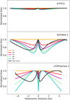 |
Fig. 1 Change in the normalized cross section of the illuminated area for three selected comet shapes (67P/C-G, 81P/Wild 2, and 103P/Hartley 2) and the sphere at five different obliquities (0°, 30°, 45°, 60°, 90°, and their real obliquity and arguments except for the sphere) with distance in au from perihelion (on a 67P/C-G-like orbit, perihelion occurs at 1.24 au). |
3 Results
3.1 Effect of shape and orientation: Model B versus Model A
To investigate how the properties of the dust layer affect orbital changes in comet water production, we employed a simplified dust layer model with a fixed thickness. Although the gas flow may remove dust particles at the upper boundary and new particles may accumulate at the lower boundary, we assume this process maintains a constant dust layer thickness. This fixed-thickness assumption provides a convenient framework for understanding the overall behavior of gas production while keeping the model computationally manageable. We did not explicitly model the dust loss rate at the upper boundary or accumulation at the lower boundary because our primary focus is comparing overall trends in water productivity with Model A.
We conducted simulations for various comets, each with different homogeneous dust layer models (listed in Table 2). The dust particle sizes were chosen based on observational data and prior studies of cometary characteristics. To reduce time costs and test the impact of dust layer existence on the evolution of the total water production rate, we used a constant grain size in our simulations. Specifically, we followed the method of Marshall et al. (2019) by analyzing changes in the exponent n in the model power-law function  , which approximates total gas productivity. Future work could incorporate a more realistic particle size distribution to improve and make our model more physically realistic.
Under the idealized assumption that all the absorbed energy is used solely for sublimation, with negligible dissipation through thermal radiation or inward heat transfer, the smallest absolute value of |n| is 2 for a spherical nucleus with a constant illuminated cross-section area. This is regarded hereafter as the Whipple model. However, in more realistic models, the mechanisms that reduce the fraction of energy available for sublimation must be considered. The deviation of |n| from 2 indirectly characterizes the role of various mechanisms for utilizing absorbed energy.
Fig. 1 summarizes the projected illuminated cross sections for the three comets studied in our simulations (67P/C-G, 81P/Wild 2, and 103P/Hartley 2) as a function of heliocentric distance. Our subsequent simulations and analysis focus on a heliocentric distance of up to 3 AU, following the approach used by Skorov et al. (2020).
In the first stage, we compare the results from Model A with those from Model B, which involves studying two types of dust particles. Specifically, we modeled porous layers consisting of micron-sized solid monomers with a particle size of 1 µm and layers with larger particles, each with a radius of about 100 µm. This choice of particle sizes aims to assess the impact of radiative heat transfer on the redistribution of absorbed energy. The characteristic particle size is directly related to the average size of voids within the layer, and this relationship holds particularly well for random layers of similarly sized particles. Consequently, the contribution of radiative transfer for layers composed of micron-sized monomers and submillimeter particles is expected to differ by approximately two orders of magnitude.
Fig. 2 illustrates the power-law exponents for the total gas production of comets 67P/C-G, 81P/Wild 2, and 103P/Hartley 2 (top to bottom) during the inbound branch as a function of heliocentric distance. The results for Model B, which uses dust layers composed of micron-sized monomers and submillimeter particles, are displayed in the left and right columns, respectively. We tested three different thicknesses for the dust layers: 3, 9, and 26 µm for the micron-sized monomers, and 0.184, 0.554, and 1.660 mm for the submillimeter particles, as shown in Table 2. Each model uses realistic orbital and spin axis orientations for the comets (see Table 1). For additional context, Fig. C.1 in Appendix C displays the inbound and outbound branches exclusively for the submillimeter particles.
In Fig. 2, the blue dash-dotted lines represent the power-law exponents for different models: the Whipple model (n ≈ −2), Model A (n ≈ −2.60), Model B (n ≈ −2.80), Model C (n ≈ −2.21), incorporating self-illumination effects based on Keller et al. (2015b), and the model introduced by Hu et al. (2017b) (n ≈ −2.85) featuring a 5 mm dust layer with a particle size of 0.5 mm. According to the ROSINA data, the exponents inbound and outbound for 67P/C-G are −5.10 and −7.15, respectively (Hansen et al. 2016).
When comparing different monomer sizes in Model B, it is clear that deviations from Model A are more pronounced for smaller particles. Additionally, the deviation increases with layer thickness; thicker layers show a greater deviation from Model A results. The minimal differences observed between hierarchical layers of varying thicknesses are likely due to their high porosity and the relatively small thickness values tested, which are insufficient to suppress gas production significantly. We note that the maximum relative thickness L/R of a layer with micron particles is twice that of a hierarchical layer.
Comparing the results between different comets demonstrates that shape and the corresponding projected cross section play more important roles than dust crust properties. For comet 67P/C-G, our results align with previous literature, not altering the established understanding. However, for comet 103P/Hartley 2, there is a clear excess over the “theoretical maximum”, likely due to the geometric increase in its cross section near perihelion rather than a physical effect.
We can formulate an intermediate conclusion: The addition of radiation thermal conductivity did not qualitatively change the overall picture. The exponent values for Model B are always slightly larger than for Model A, which is explained by the presence of thermal conductivity and the resistance of the dust crust to gas diffusion. For very finely dispersed layers, we can talk about a relative increase in the exponent with increasing layer thickness. However, the relative changes across the different layer thicknesses remain minimal for submillimeter particles.
In the second stage, we compared the results obtained with different orientations of the spin axis of the cometary nucleus (see Table 1). For Model B, we performed numerical simulations with dust layers composed of different monomer sizes but displayed results for a layer thickness of 0.184 mm for submillimeter particles. Figs. 3 and C.2 show the results for the pre- and post-perihelion branches of the orbit, respectively. The left column shows changes in the illuminated cross-section area as a function of heliocentric distance, while the right column presents corresponding changes in the exponent of the approximate power function. As expected, changes in the spin axis orientation of 67P/C-G do not lead to significant differences in the simulation results. Similar to previous results, the exponent increases slightly with greater heliocentric distance, and there is practically no difference between the inbound and outbound branches. The variation in results is comparable to the scatter caused by changes in the microscopic characteristics of the dust layer (see Fig. 3), with absolute values ranging from approximately 2.50 to 3.00.
The results for the other two comets (shown in the middle and bottom rows) are particularly interesting. The illuminated cross sections of these comets vary significantly with changes in the spin axis orientation, leading to two distinct patterns of behavior. In the first pattern, the cross section exhibits a conditional minimum – decreasing as the comet moves away from perihelion and then expanding – or a conditional maximum – increasing with distance from perihelion and then falling. For the first group, as expected, an increase in the cross-section compensates for the drop in solar energy intensity as the comet moves away from the Sun. Consequently, the exponent change for these model variants seems flatter, and the value itself approaches or even surpasses the classical value of two. Comet 103P/Hartley 2 is the best example of this, where the cross section almost doubles within a relatively small range of distances close to perihelion, resulting in an exponent smaller than unity. For these comets, the exponent tends to stabilize around two and shows little variation, even for the actual spin axis orientation (black curves).
The second pattern of behavior exhibits a significantly distinct trend. Here, the reduction in solar radiation is amplified if the cross section decreases with distance, causing the exponent to range between 4 and 5. Depending on how the nucleus cross section changes, the exponent of the function approximating gas productivity may show minimal change with increasing distance. Notably, the exponent for these two comets can vary significantly – ranging from approximately 2 to around 5 – solely due to differences in spin axis orientation. This result, which was initially proposed in the classical Whipple model (Sekanina 1981), is now confirmed through this more realistic model under analysis.
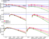 |
Fig. 2 Exponent of the power function approximating the total gas production of 67P/C-G, 81P/Wild 2, and 103P/Hartley 2 (from top to bottom) as a function of the heliocentric distance. The left and right columns depict the results with a dust layer composed of particles of size 10−4 m and 10−6 m, respectively. The corresponding layer thicknesses for these two particle sizes are provided in Table 2. The dash-dotted lines depict the power-law exponents obtained for different models utilized before and are explained in the text. The exponents of different models for 67P/C-G are shown, and corresponding values are shown in the text. |
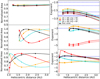 |
Fig. 3 Normalized cross section (left) and the associated exponent n of the power functions (right) for the inbound branch of 67P/C-G, 81P/Wild 2, and 103P/Hartley 2 (from top to bottom). The dust layer is built from 0.1 mm dust particles. The solid and dashed lines represent Models A and B with different obliquities and arguments (obliquity = 60°, argument = 90°; obliquity = 80°, argument = 10°; obliquity = 60°, argument = 60°; obliquity and argument = real value for real comets), respectively. The black lines correspond to the real obliquities and arguments listed in Table 1. |
3.2 Gas production and growing crust
The models discussed above assume that the dust layer thickness on the nucleus’ surface remains constant, regardless of location or heliocentric distance. These models, known as the homogeneous static dust layer, as described in Skorov et al. (2020). However, this assumption is an oversimplification. Moreover, the power-law exponents derived from these uniform static dust layers are smaller – ranging from 2 to 3 – than those estimated from Rosetta measurements for 67P/C-G, which range from 3 to 8 (Hansen et al. 2016). To address these limitations, we now consider a more sophisticated model where the dust layer thickness can vary with time.
In the previous section, we highlighted the significant impact of changes in the illuminated cross section. To focus on the effects of dust layer evolution while eliminating certain model variables, we will now consider comets where the illuminated cross section remains constant or changes very little. Specifically, we examine a spherical nucleus and the case of 67P/C-G. In our analysis, we assume zero obliquity for the spherical nucleus but use the actual spin axis for 67P/C-G.
Initially, we assume that the cometary surface is covered by a uniform monolayer of ice-free dust aggregates with a thickness of 2 mm, which corresponds to the particle size. According to Skorov et al. (2020), such a layer allows gas flow to pass through relatively easily. As the comet approaches the Sun, its activity gradually increases, leading to the sublimation of subsurface ice and a corresponding thickening of the dust layer.
In our basic model, we assume that the cohesive force between dust aggregates exceeds the gas lifting force. This assumption results in a gradual accumulation of dust as volatiles sublimate, representing the early phase of dust buildup when the comet first enters the inner solar system. As the dust layer thickens, it expands, which eventually reduces its permeability to gas flow and diminishes the evacuation of sublimation products. Over successive orbits, this process may ultimately reduce gas production, potentially contributing to the “dying” of cometary activity – a well-known and expected outcome in the life cycle of a comet.
It should be noted, however, that in regions with greater insolation and, therefore, more active dust emission, this behavior may vary significantly. In these active regions, dust removal is more efficient, which could alter the dust layer’s properties and permeability. Dust ejection in some parts of areas will be discussed further in Sect. 4.
In this study, we investigate a comet under the assumption of a thin, uniform surface layer with no significant pre-evolution during its first passage. In such a scenario, two opposing processes come into play. As a comet approaches the sun on the inbound branch, the rapid increase in insolation should boost gas production. However, the sublimation of volatiles and the accumulation of dust increase the resistance of the dust layer, potentially reducing gas production. On the outbound branch, both processes work together, likely leading to an accelerated decline in gas production.
Our theoretical analysis suggests that predicting changes in gas production on the comet’s inbound branch is challenging, even qualitatively, whereas the evolution of gas production on the outbound branch appears more predictable. We validate this observation using our numerical models. Fig. 4 shows the normalized gas production rate as a function of the heliocentric distance (left panel) and the corresponding exponent of the power law approximation (right panel) for the model with a growing layer thickness. The dust layer is composed of porous aggregates of 1 mm in diameter. Inbound and outbound orbital branches are presented for a spherical nucleus and the shape of comet 67P/C-G.
The growing dust layer model is compared to the previously discussed static dust layer model in terms of gas production. In the static model, gas production reaches a maximum at perihelion. Similarly, the growing layer model shows a rapid increase in gas production as the comet approaches perihelion. However, this increase is accompanied by a rapid thickening of the dust layer, which hinders sublimation and leads to peak gas production before perihelion.
Referring to the black curve in the upper-left panel of Figs. 3, C.2 and 4, we see that for the inbound branch (RH > 1.6 au), the exponent changes for both the growing layer model and the static layer model are comparable, with their exponents ranging between 2 and 3. However, as the comet approaches perihelion, the behavior of the exponents in the static dust layer model and growing dust layer model begins to differ significantly. This qualitative divergence is evident when comparing the variation of the exponents for 67P/C-G (in the left panel of Fig. 4 and in the top panel for 67P/C-G in Fig. C.1). In the growing layer model, gas production levels off quickly for both the spherical nucleus and 67P/C-G. The exponents decrease progressively, approaching 0 around 1.25 au, corresponding to unchanged gas production in the left panel of Fig. 4. In this case, the increase in insolation is almost completely damped by a decrease in layer permeability. This specific behavior within the growing dust layer model is observed in our model for the first time.
In the vicinity of perihelion, there is a small region where gas production slightly decreases as the comet gets closer to the Sun. This effect is unexpected since insolation typically increases with decreasing distance. This non-monotonic behavior is observed for both nucleus shapes, and the region where production decreases corresponds to positive values of the exponent in our approximating power function.
The stark contrast between gas production on the inbound and outbound branches, as well as the behavior of the exponent, is notable and differs sharply from the static model B, where there is no significant difference in results before and after perihelion (Fig. C.1). In the post-perihelion stage, the growth rate of the dust layer thickness slows, but it continues to decrease the exponent of gas production.
Although the cross-section curves for the spherical nucleus and 67P/C-G are similar, 67P/C-G’s bilobed shape and oblique spin axis lead to nonuniform illumination across its surface. For the spherical comet, the dust layer thickness depends only on latitude and is symmetrical around the equator. In contrast, for 67P/C-G, the insolation is distributed much more unevenly, leading to highly heterogeneous and asymmetrical crust growth. As a result, Fig. 4 demonstrates the notably different gas production curves for the cases with near-constant cross sections.
To observe local dust layer changes, we plotted the thickness variation for five facets on the spherical nucleus, as shown in Fig. 5. The surface of the sphere was divided into five latitude intervals (specifically: [−90°, −50°], [−50°, −20°], [−20°, 20°], [20°, 50°], [50°, 90°]). One facet was randomly selected from each band, each receiving different levels of insolation. The initial dust layer thickness was 2 mm uniformly, with aggregate sizes of 1 mm. The left and right columns illustrate the cumulative crust thickness in the pre- and post-perihelion branches, respectively.
Differences in dust layer thickness between facets are already noticeable at 3 au, with up to a three-fold increase at lower latitudes, leading to some suppression of gas production in the sub-equatorial region. Compared to Model A and Model B with a fixed dust layer, the growing dust layer model shows less heterogeneity in local gas production at large heliocentric distances. However, as the comet nears perihelion, the dust layer differences decrease to about 1.5 times. Despite the reduced thickness variation, gas production heterogeneity increases near perihelion. This increase is attributed to enhanced insolation that amplifies local variations in activity, outweighing the homogenizing effect of the thinner dust layers.
The local gas production rate Z for the selected facets is shown in Fig. 6, with the left and right panels representing the inbound and outbound branches. Except for one facet in the “polar” region (represented by the lowest prasinous curve), the other facets form a relatively tight group, displaying very similar behavior. This similarity becomes even more pronounced as the comet moves away from the Sun. Near perihelion, we observe a slight divergence of the curves and a noticeable decrease in production with decreasing distance, an effect visible in all control areas except the polar one.
Unlike the spherical nucleus, the situation for 67P/C-G is much more complex, making numerical modeling essential. To characterize the behavior of different regions on the nucleus surface, we selected five facets as shown in Fig. 7. The selection of these facets is guided by two criteria: the nature of the local surface materials and the intensity of solar radiation received in these regions. Regarding surface material heterogeneity, we focus on dust-covered terrains, brittle materials, large-scale depressions, and smooth terrains. Within the dust-covered regions, we specifically targeted facets exposed to the highest levels of solar radiation. This methodical selection ensures our analysis focuses on regions where solar energy significantly influences dust layer evolution.
The top panel in Fig. 8 presents the variation in solar flux, dust layer thickness, and production rate for the selected facets. Table 3 provides the locations of the selected facets on the surface of 67P/C-G. The upper panel shows solar flux variation as a function of heliocentric distance for the tested facets, revealing three distinct groups: (1) Southern hemisphere (Anubis and Imhotep regions): In this group, solar flux increases as the nucleus approaches the Sun, leading to a relatively rapid dust layer growth, which becomes explosive near the perihelion. (2) Equatorial region of the small lobe (Nut and Hatmehit regions): Here, insolation changes non-monotonically, with a slight initial increase, peaking between 2 and 1.5 au, followed by a sharp decline. (3) Northern hemisphere (Hapi, Babi, and Ma’at regions): For these facets, solar flux changes little until a distance of 2 au, after which it decreases monotonically as perihelion approaches. These patterns generally persist in the post-perihelion branch (right panel).
Since the entire evolution of the surface is driven by the redistribution of absorbed solar energy, it is insightful to compare the changes in gas production (middle row in Fig. 8) with the buildup of the dust layer (bottom row in Fig. 8). Due to the seasonal effect caused by the spin axis orientation, the facets in the Anubis and Imhotep regions experience progressive illumination, leading to a noticeable increase in activity after the vernal equinox. While the insolation curves for these facets show a gradual increase, the gas production curves rise more sharply as the comet approaches the Sun. Both facets exhibit characteristic inflection points, with gas production decreasing just before perihelion.
A similar effect – where the maximum gas production is slightly shifted – is also observed in Fig. 6. This effect cannot be understood without consideration of the growth of the dust crust. The rapid increase in the layer thickness for these areas leads to a partial suppression of gas production near the perihelion. Consequently, the behavior of these curves resembles that observed from the spherical nucleus. However, unlike the spherical nucleus, the solar flux in the Anubis and Imhotep regions does not grow uniformly; instead, it surges suddenly before perihelion. At 3 AU, the dust layer shows little change, but following this sudden flux increase, it rapidly thickens to 0.05 m, effectively suppressing gas production near the perihelion. After perihelion, as gas production declines rapidly, the dust layer thickness in these regions stabilizes at around 25–30 particle sizes after the autumn equinox. At this point, cometary activity significantly diminishes.
The facets within the Nut and Hatmehit regions, located on the small lobe near the equator, experience fluctuating insolation that peaks before perihelion, drops to its lowest point, and then gradually increases after perihelion. This pattern results in similar gas production curves and a smooth, gradual growth of the dust layer. On the outbound branch, although the heliocentric distance increases, the insolation remains relatively stable at a low level compared to the rapid changes before perihelion. This leads to a minimal gas production rate and slower dust layer growth, with the dust layer thickness remaining approximately half that of the previously mentioned regions.
This effect is even more pronounced for facets in the Hapi, Babi, and Ma’at regions, located in the northern hemisphere (as shown in Fig. 7). The facets in the Hapi and Babi regions fall into shadow shortly before perihelion, while the facet in the Ma’at region stops receiving solar radiation at distances closer than about 1.5 au. Before entering shadow, the insolation in these regions remains relatively constant, around 100 W/m2. This low level of energy is sufficient only for a modest gas production rate of less than 1020 molec/s/m2 and a slow increase in the thickness of the dust layer. Although the layer grows more slowly than in the Nut and Hatmehit regions, it still becomes thicker than the layers in the Anubis and Imhotep regions around 3 AU. However, as the Anubis and Imhotep regions enter their phase of explosive growth, the northern regions, receiving less illumination due to seasonal effects, experience a natural halt in dust growth. After the autumn equinox, when parts of the northern regions are illuminated again, the dust layer thickness shows little further increase. This stagnation is due to both the presence of the existing dust layer and the insufficient solar radiation energy available to drive further growth.
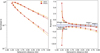 |
Fig. 4 Normalized gas production (left panel) and exponent of the power-law model (right panel) are shown for models of spherical nucleus and 67P/C-G with a quasi-constant cross section. Gas production is calculated in Model B with growing layer thickness. The dust particle size is 10−3 m and the initial dust layer thickness is 2 × 10⁻³ m. The effective layer porosity is about 85%. The solid and dashed lines represent pre- and post-perihelion branches, respectively. |
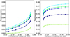 |
Fig. 5 Variation of the dust layer thickness as a function of the heliocentric distance for the sphere is estimated in Model B. The aggregate size is 10−3 m and the initial dust layer thickness is 2 × 10⁻³ m. The left and right panels represent the cumulative thicknesses at pre- and postperihelion branches, respectively. The results shown are for five surface facets at different latitudes on the sphere. See more details in the text. |
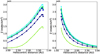 |
Fig. 6 Gas production rate of the selected facets in Fig. 5 as a function of the heliocentric distance. The left and right panels represent the results for pre- and post-perihelion branches, respectively. |
Region, latitude, longitude, and hemisphere of the facets of 67P/C-G used in this study.
 |
Fig. 7 Location of selecting facets from different regions of 67P/C-G: Hatmehit, Nut, Hapi, Babi, Ma’at, Anubis, and Imhotep. |
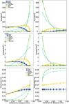 |
Fig. 8 Heliocentric evolution of key physical model characteristics for the five selected facets on 67P/C-G; the solar flux (top), the gas production rate (middle), and the dust layer thickness (bottom) are shown as functions of heliocentric distance. The left and right columns represent pre- and post-perihelion branches, respectively. |
4 Discussion
In the previous section, we introduced results from the dust layer growing model, which simulates the evolution of the dust layer due to volatile sublimation. This model revealed new insights, such as strong asymmetries in gas production between the inbound and outbound branches and a flattening of the production curve near perihelion. We also highlighted that these scenarios represent the “first entry” of a comet into the inner solar system, where active sublimation of water ice begins. The dust layer growing model assumes that the remaining dust after ice removal forms a dry crust on the comet’s surface, held together by cohesive forces between particles (Skorov & Blum 2012). This scenario describes the so-called “secular death” of some regions, where activity gradually diminishes with each subsequent orbit, leading to a transition to an inactive state.
To overcome the limitation of this simplistic assumption and introduce dust removal, we consider a model in which the vapor pressure beneath the dust layer can exceed the tensile strength of the material. Many researchers have simplified this scenario by ignoring the material’s tensile strength and instead used a simplified relationship between gravitational force and lift force from gas flow (e.g., Rickman et al. 1990; Gundlach et al. 2015). This approach is more applicable when considering isolated particles on the surface rather than a thick porous layer.
Based on our dust layer growing model, we now include a new control mechanism to account for dust removal. Specifically, at each time step, we compare the lift force acting on the dust layer with its tensile strength. The lift force is estimated based on the vapor pressure at the lower boundary of the layer (Marshall et al. 2019), given by:
 (1)
(1)
where T represents the temperature at the lower boundary of the dust layer, which is determined by the local insolation and energy balance. For the tensile strength of the dust layer, we use the formula provided in Skorov & Blum (2012)
 (2)
(2)
where ϕ is the volume filling factor due to the packing structure of the dust layer. Assuming ϕP = 0.4, the effective tensile strength Teff is calculated to be 0.64 Pa for dust aggregates with a radius r = 1 mm. If the vapor pressure P(T) exceeds the tensile strength Teff of the dust layer (P(T) > Teff ), the dust layer is considered to be completely removed, leading to a new cycle of dust accumulation.
Our model incorporates certain simplifications to ensure computational efficiency. Notably, we assume that the tensile strength of the dust layer remains consistent across both dry and icy regions. While actual cometary materials likely exhibit more complex behavior due to heterogeneous properties and local variability, we assume each facet is homogeneous. This approach enables us to avoid the need to account for partial removal of material.
The results of modeling gas production and the corresponding exponent as a function of heliocentric distance are shown in Fig. 9. For the idealized model, we observe that at distances of approximately 1.50–1.75 au, partial dust layer discharge occurs: gas production accelerates, and the exponent changes from values typical of fixed or growing layer thicknesses to significantly larger values. These simulated exponent values are in good agreement with observational estimates near perihelion, suggesting that our model is moving in the right direction.
Two additional preliminary conclusions emerge from analyzing the exponent near perihelion. First, both the inbound and outbound branches show kinks in the curve, reflecting short-term cycles of dust layer accumulation and discharge. This behavior aligns with earlier proposals made in Skorov & Blum (2012), and recent results from Skorov et al. (2024b) further support the possibility of these repeated discharges. Second, we observe a general trend of increasing exponent values for the outbound branches, which is consistent with observational trends.
Finally, it is also important to note that dust layer discharge does not occur uniformly across the spherical nucleus. Our analysis shows that the dust layer in the equatorial region is ejected first and undergoes the most cycles. At higher latitudes, the solar flux decreases, leading to a delay in dust emission and a reduction in discharge frequency. In latitudes above 50°, the dust layer continues to accumulate rather than being discharged. Fig. 10 illustrates this, presenting dust layer thickness and water production rates at different heliocentric distances (5.683 au, 2.777 au, and 1.243 au) from left to right. Each panel shows variations in these parameters along the latitude of the sphere, with the vertical axis representing latitude and the horizontal axis representing dust layer thickness or water production rate. This figure intuitively depicts the dynamic evolution of the global dust layer thickness at initial, intermediate, and perihelion distances. Near perihelion, surface facets at latitudes below 50° have undergone dust layer ejection.
As in Sect. 3.2, we selected five facets at different latitudes to analyze the evolution of the dust layer and the corresponding water production rate as a function of heliocentric distance using the dust layer removal model (Figs. 11 and 12). For the three facets where dust ejection occurred, the removal process started at different heliocentric distances, with the equatorial facets losing their dust first. This ejection happened multiple times near perihelion. As the comet approached perihelion, the maximum dust layer thickness that a facet could accumulate gradually decreased, resulting in a step-like distribution.
In summary, both temporal and spatial heterogeneity in gas production were evident. The initially homogeneous global dust layer evolved into a complex structure. Low-latitude regions experienced multiple discharges, while high-latitude regions mainly underwent dust accumulation. These effects likely increase the heterogeneity of gas production across the comet’s surface. Consequently, the processes discussed here should significantly influence the reactive forces generated by ice sublimation, which in turn could cause nongravitational perturbations in the comet’s orbital motion. This issue will also be the focus of our next work.
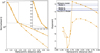 |
Fig. 9 Change of the normalized gas production rate (left column) and exponent of the model power function (right column) as a function of heliocentric distance for a comet of spherical shape and 67P/C-G. The dust particles are 10−3 m and the initial layer thickness is 2 × 10⁻³ m. |
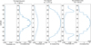 |
Fig. 10 Dust layer thickness and gas production rate for several orbital positions, the beginning point (at aphelion), the midpoint between the beginning and perihelion points, and the perihelion point from left to right. The corresponding heliocentric distance for each point is shown. |
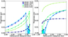 |
Fig. 11 Variation in the thickness under the dust layer removal model is presented as a function of heliocentric distance for a comet with a spherical shape. Facets situated at different latitudes are examined, as legend shows. This permits the identification of latitudes where the dust layer has been removed. |
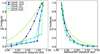 |
Fig. 12 This figure complements Fig. 11, showcasing the gas production rate of the selected facets as a function of heliocentric distance. |
5 Conclusions
Using a two-layer thermophysical model, we investigated the sensitivity of heliocentric water production curves to several surface parameters, including dust layer thickness and particle size. We also analyzed the impact of the dynamically evolving dust layer on water production variation.
The following general conclusions can be drawn from the presented results:
The homogeneous two-layer outgassing model, with fixed layer characteristics, showed only minor qualitative differences from simpler models of water ice sublimation driven by solar insolation. This suggests that while more complex models provide deeper insights, simpler models are still effective in illustrating the strong dependence of cometary activity on the illuminated cross-section area. However, our results emphasize the extent to which spin axis orientation and comet shape influence the total gas production rates of active comets, providing a more detailed understanding of these factors in determining cometary outgassing;
Comparing spherical nucleus models and the specific shape model of comet 67P/C-G, we found that scenarios with dust accumulation and continuous growth of layer thickness resulted in exponents that significantly differed from those produced by models with static dust layers. The dust layer growing model revealed noticeable asymmetry in the water production rate curve around the perihelion. As shown in Fig. 4, the accumulation of dust layer thickness suppressed gas production, leading to a decrease in the water production rate as the heliocentric distance decreased near perihelion. This scenario allowed for a wide range of exponents, from 2 to 6, depending on the initial dust layer thickness. The variability highlights the importance of incorporating dynamic dust layer models for a better understanding of cometary activity, particularly to represent the impact of dust buildup on gas production;
The possibility of local removal of the dust layer near perihelion due to uneven heating was demonstrated by including tensile strength in a homogeneous spherical nucleus model. This finding suggests that physical interactions within the dust layer significantly impact observed gas production rates. In contrast to models without crust removal, the exponents in this scenario exhibited distinct behavior, reaching values around 7–8 near perihelion. Dust ejection was observed predominantly in low-latitude regions, while high-latitude regions primarily experienced dust accumulation. This scenario emphasizes the pronounced temporal and spatial heterogeneity of gas production, highlighting the importance of incorporating nongravitational effects during dust removal in future research.
Simulating the dynamic process of comet sublimation is highly complex and requires considering numerous factors, many of which remain uncertain. Although the illuminated cross-section areas and global water production rate curves for 67P/C-G and a spherical nucleus may appear similar when averaged over large scales, significant local variations play an essential role in shaping the specific features of cometary outgassing. Thus, while a spherical model may provide a useful approximation of overall comet activity, it fails to capture the detailed behavior that arises from individual facets.
For instance, seasonal effects cause stark differences in illumination levels between the northern and southern hemispheres of 67P/C-G. The northern hemisphere experiences relatively mild insolation, resulting in weak dust removal, whereas the southern hemisphere, exposed to intense sunlight, undergoes substantial dust ejection. Even within the southern hemisphere, individual facets respond differently to local insolation at different heliocentric distances, leading to divergent dust dynamics, gas production rates, and nongravitational effects.
Therefore, accurate simulations of comet activity must account for these local facet-specific conditions by incorporating detailed shape and morphology data. This approach is crucial to realistically modeling the processes that drive cometary outgassing and the associated nongravitational forces, providing a more comprehensive understanding of comet evolution and behavior.
Data availability
The data underlying this article will be shared on reasonable request with the corresponding author.
Acknowledgements
We thank H.U. Keller for his encouragement and helpful discussions. YX and YZ were supported by the National Natural Science Foundation of China (Grant Nos. 12222307, 12073084). YS acknowledges support from ESA through contract 4000141229/23/ES/CM and the Deutsche Forschungsge- meinschaft (DFG) for support under grant BL 298/32-1, and the CAS PIFI project (Grant No. 2022VMB0010). LR acknowledges support from the project DFG-392267849.
Appendix A Microscopic model of gas production
The microscopic thermophysical model used in this study includes two main components. The first component is responsible for generating a random porous layer and calculating the resistance to free molecular diffusion through this layer. In this study, the building unit of the model is a dense porous aggregate composed of uniformly sized spheres. The second component focuses on heat transfer within the model layer, enabling the calculation of effective gas production during the sublimation of ice located beneath the surface crust.
To simulate gas passage through the layer, we employ the Test Particle Monte Carlo (TPMC) method (Skorov et al. 2011). This method assumes that gas particles do not undergo inter- molecular collisions and that they scatter diffusely only upon interacting with dust particles. This assumption implies a collisionless gas flow, which is generally valid when the Knudsen number (the ratio of the mean free path MFP in an equilibrium gas to the characteristic size of the system) is approximately 10 or greater.
In practice, the pore size or void size in the layer is typically used as the characteristic size. The validity of this approach for our scenarios has been demonstrated in Skorov et al. (2024a), where a more sophisticated Direct Simulation Monte Carlo (DSMC) model was used to study gas flow. For the expected temperature ranges (T ~ 200K), the collisionless flow assumption holds true for particles up to the millimeter scale.
In our study, we utilize several key characteristics of the porous layer: its effective porosity ϕ, the layer’s permeability to gas flow Π, and the mean free path MFP. The mean free path serves as the characteristic void size (Macher et al. 2024). Porosity and permeability, along with the layer’s thickness, are directly incorporated into the thermal model equations. The mean free path affects the effective thermal conductivity, determining the radiative term’s input.
A one-dimensional two-layer thermophysical model is applied to simulate heat transfer and ice sublimation under a porous dust crust. In this model, a porous layer composed of a mixture of ice and dust is covered by a second porous layer made entirely of dry dust. The model operates under the assumption that the temperature distribution within the top surface layer of a slowly rotating comet is quasi-stationary. This assumption allows the heat conduction equation to be analyzed under a stationary approximation.
The resulting model comprises a closed system of two nonlinear algebraic equations, which are solved for two variables: the surface temperature Ts and the temperature at the sublimation front Ti . These equations precisely represent the energy balances within the system.
Given the high porosity and large particle size of the surface layer, direct solar radiation penetrates to a significant depth. This penetration introduces a volumetric energy source term into the heat transport equation. Therefore, the stationary heat equation, incorporating this energy source term Q(x) to account for the absorption of direct solar radiative flux (or insolation) at depth, is expressed as:
 (A.1)
(A.1)
where T(x) is the temperature distribution as a function of depth x, and Keff is the effective thermal conductivity of the layer.
To estimate the volume energy absorption (VEA) term Q(x) and achieve an acceptable parameterization for simulations, we used the TPMC method, the Dense Medium Radiative Transfer (DMRT) theory (Tsang 1985), and the fast superposition T-matrix method (FaSTMM) (Markkanen & Yuffa 2017).
The boundary conditions for energy conservation at the cometary surface and at the interface between the dust layer and the underlying ice are as follows:
 (A.2)
(A.2)
 (A.3)
(A.3)
where Ieff is the effective absorbed solar irradiation, ϵ is the emissivity, σ is the Stefan-Boltzmann constant, Z is the sublimation rate, H is the latent sublimation heat, and Π is the layer gas permeability, which is a function of the layer thickness, porosity, and particle size. The sublimation rate is given by the Hertz-Knudsen formula, Z(T) = P(T)/(0.5πvth), where P(T) is the saturation vapor pressure,  is the thermal velocity of the vapor molecules, and µ is the molar mass. The variables Keff (T) and
  are the effective heat conductivities of the porous dust layer and the icy medium, respectively.
These boundary conditions incorporate energy absorption and emission at the cometary surface and account for heat transfer across the dust-ice interface. The provided formulas account for the fact that the solid phase responsible for energy absorption and emission occupies only a portion of the outer boundary in the model of a homogeneous porous layer. The volume ratio of dust to ice is unity, implying that the filling factor of the icy region is twice that of the dry dust layer. Although there is a difference in the thermal conductivities of dust and ice, it is considered negligible in this analysis due to their small values and minimal effect on the heat flux to the interior. For a detailed discussion on this approximation, refer to Skorov et al. (2024a).
In Model B, the gas flow rate is influenced by the permeability Π and the effective thermal conductivity Keff, which include both the conductive and radiative components. The radiative component of the thermal conductivity, Kr , depends on temperature and follows a relationship approximately proportional to T4. This approach shares a similar complexity with models used by Hu et al. (2017a) and Gundlach et al. (2020). For a comprehensive understanding of this model, including its equations and limitations, we refer readers to the works of Skorov et al. (2022), Skorov et al. (2023b), and Skorov et al. (2023a). With a comparable degree of realism in the physical description, Model B is significantly faster than models accounting for unsteady heat transfer. This computational efficiency is one of the most important advantages, allowing for extensive pre-calculations across a wide range of parameters. These pre-calculated results can be integrated into more detailed models that examine complex features such as the intricate shape of the cometary nucleus (Skorov et al. 2024a) or the orbital motion and integration over the surface (as done here). The solid thermal conductivity is calculated using the method proposed by Gundlach & Blum (2012), while the radiative thermal conductivity is derived from the results presented by Skorov et al. (2023b). For our simulations of water-ice sublimation, we use the constants listed in Table A.1.
Model values for ice and thermal conductivity
Appendix B Macroscopic model of gas production
B.1 Total production simulation
The total illuminated cross-section area A of a comet is defined as the sum of all active facets:
 (B.1)
(B.1)
where Ak is the area of the kth facet and θk is the angle between the facet normal vector and the vector from the facet center to the Sun. If θk is greater than 90°, the facet is considered nonilluminated. In such cases, θk is set to 90°, which results in zero flux for that facet. Non-illuminated facets are thus considered inactive in the model.
We consider several scenarios for the evolution of the nucleus with fixed, growing, and removal dust layers. For the fixed dust layer scenario, we use the microscopic gas production model described in Appendix A to compute the change in gas production rate with heliocentric distance for various dust layer properties. We then determine the local solar flux Fk for each facet based on its orbital position and rotational state. The flux is calculated as follows:
 (B.2)
(B.2)
where S⊙ is the solar flux with a value of 1367 W m−2 at 1 au and Rh is the heliocentric distance. Note the Bond albedo in Eq. B.2 is neglected in this model (Lamy et al. 2007). The comet’s orbit is divided into norb intervals, each corresponding to an equal change in the eccentric anomaly ΔE = 2π/norb. Each orbital interval corresponds to a single rotation in both the static and growing dust layer models. Additionally, the rotation period is divided into nrot steps. Within each orbital interval, the sublimation rate  for facet k during the j-th rotation step is calculated based on the solar flux for the i-th orbital interval.
The average sublimation rate for facet k at the heliocentric distance Rh , assumed constant within the i-th orbital interval, is given by:
 (B.3)
(B.3)
The global water production rate at heliocentric distance Rh is the product of the average sublimation rate  and the facet area Ak :
 (B.4)
(B.4)
where N is the total number of active facets.
B.2 Growing dust layer modeling
In the scenario with a growing dust layer, we calculate the thickness increase of the dust layer based on the water production rate at each orbital step. We assume a dust-to-water-ice density ratio of 3:1. The growth of the dust layer is determined by integrating the dust accumulation throughout an orbital revolution.
The orbit period is divided into norb intervals, each with an equal change of eccentric anomaly. The duration  of the i-th orbital step can be derived from the relative mean anomaly change ΔMi (Zhao et al. 2020). The duration of each rotation step for the i-th orbit step is
  . For each facet k, the total gas production
  during the i-th orbital interval is calculated by summing the production across all rotation steps:
 (B.5)
(B.5)
Next, we obtain the increase  in erosion depth of the facet k during the i-th orbital interval:
 (B.6)
(B.6)
where  is the density of water ice.
Given the dust-to-water-ice density ratio of 3:1, the thickness of the accumulated dust layer is:
 (B.7)
(B.7)
Appendix C Supplementary figures
This appendix includes supplementary figures as support materials for this paper.
Fig. C.1 shows the exponents for different comet models—67P/C-G, 81P/Wild 2, and 103P/Hartley 2—dis- played from top to bottom as a function of heliocentric distance. In this figure, Model B is shown with dust layer thicknesses of L1 = 0.184 mm, L2 = 0.554 mm, and L3 = 0.166 mm for submillimeter dust particles. The left and right columns correspond to the inbound (pre-perihelion) and outbound (post-perihelion) branches, respectively.
Fig. C.2 shows the simulation results for the post-perihelion branch. The left column illustrates the variation of the illuminated cross-section area, while the right column shows the corresponding exponent as a function of heliocentric distance. The solid and dotted lines represent the results of Model A and Model B, respectively, assuming in the latter case that the dust layer thickness composed of submillimeter particles is 0.184 mm.
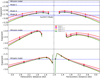 |
Fig. C.1 Exponent for the power functions approximating the total gas production of 67P/C-G, 81P/Wild 2, and 103P/Hartley 2 (from top to bottom) as a function of heliocentric distance. L1, L2, and L3 represent the thicknesses of the dust layer in Model B, composed of dust particles with a size of 10−4 m. The left and right columns correspond to pre- and post-perihelion conditions, respectively. |
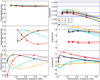 |
Fig. C.2 Same as Fig. 3 but for postperihelion. The left column shows the variation in the illuminated cross-section area, while the right column presents the corresponding exponent as a function of heliocentric distance. Solid and dotted lines represent Model A and Model B results, respectively, for a dust layer thickness of 0.184 mm composed of submillimeter particles. |
References
- Fanale, F. P., & Salvail, J. R. 1984, Icarus, 60, 476 [NASA ADS] [CrossRef] [Google Scholar]
- Fink, U., & Rubin, M. 2012, Icarus, 221, 721 [NASA ADS] [CrossRef] [Google Scholar]
- Gundlach, B., & Blum, J. 2012, Icarus, 219, 618 [CrossRef] [Google Scholar]
- Gundlach, B., Blum, J., Keller, H. U., & Skorov, Y. V. 2015, A&A, 583, A12 [NASA ADS] [CrossRef] [EDP Sciences] [Google Scholar]
- Gundlach, B., Fulle, M., & Blum, J. 2020, MNRAS, 493, 3690 [NASA ADS] [CrossRef] [Google Scholar]
- Hansen, K. C., Altwegg, K., Berthelier, J.-J., et al. 2016, MNRAS, 462, S491 [Google Scholar]
- Herique, A., Kofman, W., Zine, S., et al. 2019, A&A, 630, A6 [NASA ADS] [CrossRef] [EDP Sciences] [Google Scholar]
- Hu, X., Shi, X., Sierks, H., et al. 2017a, MNRAS, 469, S295 [NASA ADS] [CrossRef] [Google Scholar]
- Hu, X., Shi, X., Sierks, H., et al. 2017b, A&A, 604, A114 [NASA ADS] [CrossRef] [EDP Sciences] [Google Scholar]
- Ivanova, O., Reshetnyk, V., Skorov, Y., et al. 2018, Icarus, 313, 1 [Google Scholar]
- Keller, H. U., Mottola, S., Skorov, Y., & Jorda, L. 2015a, A&A, 579, L5 [NASA ADS] [CrossRef] [EDP Sciences] [Google Scholar]
- Keller, H. U., Mottola, S., Davidsson, B., et al. 2015b, A&A, 583, A34 [NASA ADS] [CrossRef] [EDP Sciences] [Google Scholar]
- Keller, H. U., Mottola, S., Hviid, S. F., et al. 2017, MNRAS, 469, S357 [Google Scholar]
- Lamy, P. L., Toth, I., Davidsson, B. J. R., et al. 2007, Space Sci. Rev., 128, 23 [CrossRef] [Google Scholar]
- Liu, C., Zhao, Y., & Ji, J. 2023, Acta Astron. Sin., 64, 11 [Google Scholar]
- Macher, W., Skorov, Y., Kargl, G., Laddha, S., & Zivithal, S. 2024, J. Eng. Math., 144, 2 [NASA ADS] [CrossRef] [Google Scholar]
- Markkanen, J., & Yuffa, A. J. 2017, JQSRT, 189, 181 [NASA ADS] [CrossRef] [Google Scholar]
- Marshall, D., Rezac, L., Hartogh, P., Zhao, Y., & Attree, N. 2019, A&A, 623, A120 [NASA ADS] [CrossRef] [EDP Sciences] [Google Scholar]
- Pätzold, M., Andert, T. P., Hahn, M., et al. 2019, MNRAS, 483, 2337 [CrossRef] [Google Scholar]
- Preusker, F., Scholten, F., Matz, K.-D., et al. 2017, A&A, 607, L1 [NASA ADS] [CrossRef] [EDP Sciences] [Google Scholar]
- Rickman, H., Fernandez, J. A., & Gustafson, B. S. 1990, A&A, 237, 524 [Google Scholar]
- Sekanina, Z. 1981, Annu. Rev. Earth Planet. Sci., 9, 113 [CrossRef] [Google Scholar]
- Skorov, Y., & Blum, J. 2012, Icarus, 221, 1 [Google Scholar]
- Skorov, Y., van Lieshout, R., Blum, J., & Keller, H. U. 2011, Icarus, 212, 867 [NASA ADS] [CrossRef] [Google Scholar]
- Skorov, Y., Rezac, L., Hartogh, P., & Keller, H. U. 2017, A&A, 600, A142 [NASA ADS] [CrossRef] [EDP Sciences] [Google Scholar]
- Skorov, Y., Reshetnyk, V., Rezac, L., et al. 2018, MNRAS, 477, 4896 [NASA ADS] [CrossRef] [Google Scholar]
- Skorov, Y., Keller, H. U., Mottola, S., & Hartogh, P. 2020, MNRAS, 494, 3310 [NASA ADS] [CrossRef] [Google Scholar]
- Skorov, Y., Reshetnyk, V., Bentley, M., et al. 2021, MNRAS, 501, 2635 [CrossRef] [Google Scholar]
- Skorov, Y., Reshetnyk, V., Bentley, M. S., et al. 2022, MNRAS, 510, 5520 [NASA ADS] [CrossRef] [Google Scholar]
- Skorov, Y., Markkanen, J., Reshetnyk, V., et al. 2023a, MNRAS, 522, 4781 [NASA ADS] [CrossRef] [Google Scholar]
- Skorov, Y., Reshetnyk, V., Küppers, M., et al. 2023b, MNRAS, 519, 59 [Google Scholar]
- Skorov, Y., Reshetnyk, V., Markkanen, J., et al. 2024a, MNRAS, 527, 12268 [Google Scholar]
- Skorov, Y. V., Mokhtari, O., Macher, W., et al. 2024b, A&A, 689, A131 [NASA ADS] [CrossRef] [EDP Sciences] [Google Scholar]
- Tsang, L. 1985, Theory of Microwave Remote Sensing, Wiley Series in Remote Sensing (New York: Wiley) [Google Scholar]
- Whipple, F. L. 1950, Astrophys. J., 111, 375 [NASA ADS] [CrossRef] [Google Scholar]
- Zhao, Y., Rezac, L., Skorov, Y., & Li, J. Y. 2020, MNRAS, 492, 5152 [Google Scholar]
- Zhao, Y., Rezac, L., Skorov, Y., et al. 2021, Nat. Astron., 5, 139 [Google Scholar]
All Tables
Semi-major axis (a), eccentricity (e), obliquity (θ), arguments (ω), and facets number (N) of comets used in this study.
Region, latitude, longitude, and hemisphere of the facets of 67P/C-G used in this study.
All Figures
|
Fig. 1 Change in the normalized cross section of the illuminated area for three selected comet shapes (67P/C-G, 81P/Wild 2, and 103P/Hartley 2) and the sphere at five different obliquities (0°, 30°, 45°, 60°, 90°, and their real obliquity and arguments except for the sphere) with distance in au from perihelion (on a 67P/C-G-like orbit, perihelion occurs at 1.24 au). |
| In the text | |
|
Fig. 2 Exponent of the power function approximating the total gas production of 67P/C-G, 81P/Wild 2, and 103P/Hartley 2 (from top to bottom) as a function of the heliocentric distance. The left and right columns depict the results with a dust layer composed of particles of size 10−4 m and 10−6 m, respectively. The corresponding layer thicknesses for these two particle sizes are provided in Table 2. The dash-dotted lines depict the power-law exponents obtained for different models utilized before and are explained in the text. The exponents of different models for 67P/C-G are shown, and corresponding values are shown in the text. |
| In the text | |
|
Fig. 3 Normalized cross section (left) and the associated exponent n of the power functions (right) for the inbound branch of 67P/C-G, 81P/Wild 2, and 103P/Hartley 2 (from top to bottom). The dust layer is built from 0.1 mm dust particles. The solid and dashed lines represent Models A and B with different obliquities and arguments (obliquity = 60°, argument = 90°; obliquity = 80°, argument = 10°; obliquity = 60°, argument = 60°; obliquity and argument = real value for real comets), respectively. The black lines correspond to the real obliquities and arguments listed in Table 1. |
| In the text | |
|
Fig. 4 Normalized gas production (left panel) and exponent of the power-law model (right panel) are shown for models of spherical nucleus and 67P/C-G with a quasi-constant cross section. Gas production is calculated in Model B with growing layer thickness. The dust particle size is 10−3 m and the initial dust layer thickness is 2 × 10⁻³ m. The effective layer porosity is about 85%. The solid and dashed lines represent pre- and post-perihelion branches, respectively. |
| In the text | |
|
Fig. 5 Variation of the dust layer thickness as a function of the heliocentric distance for the sphere is estimated in Model B. The aggregate size is 10−3 m and the initial dust layer thickness is 2 × 10⁻³ m. The left and right panels represent the cumulative thicknesses at pre- and postperihelion branches, respectively. The results shown are for five surface facets at different latitudes on the sphere. See more details in the text. |
| In the text | |
|
Fig. 6 Gas production rate of the selected facets in Fig. 5 as a function of the heliocentric distance. The left and right panels represent the results for pre- and post-perihelion branches, respectively. |
| In the text | |
|
Fig. 7 Location of selecting facets from different regions of 67P/C-G: Hatmehit, Nut, Hapi, Babi, Ma’at, Anubis, and Imhotep. |
| In the text | |
|
Fig. 8 Heliocentric evolution of key physical model characteristics for the five selected facets on 67P/C-G; the solar flux (top), the gas production rate (middle), and the dust layer thickness (bottom) are shown as functions of heliocentric distance. The left and right columns represent pre- and post-perihelion branches, respectively. |
| In the text | |
|
Fig. 9 Change of the normalized gas production rate (left column) and exponent of the model power function (right column) as a function of heliocentric distance for a comet of spherical shape and 67P/C-G. The dust particles are 10−3 m and the initial layer thickness is 2 × 10⁻³ m. |
| In the text | |
|
Fig. 10 Dust layer thickness and gas production rate for several orbital positions, the beginning point (at aphelion), the midpoint between the beginning and perihelion points, and the perihelion point from left to right. The corresponding heliocentric distance for each point is shown. |
| In the text | |
|
Fig. 11 Variation in the thickness under the dust layer removal model is presented as a function of heliocentric distance for a comet with a spherical shape. Facets situated at different latitudes are examined, as legend shows. This permits the identification of latitudes where the dust layer has been removed. |
| In the text | |
|
Fig. 12 This figure complements Fig. 11, showcasing the gas production rate of the selected facets as a function of heliocentric distance. |
| In the text | |
|
Fig. C.1 Exponent for the power functions approximating the total gas production of 67P/C-G, 81P/Wild 2, and 103P/Hartley 2 (from top to bottom) as a function of heliocentric distance. L1, L2, and L3 represent the thicknesses of the dust layer in Model B, composed of dust particles with a size of 10−4 m. The left and right columns correspond to pre- and post-perihelion conditions, respectively. |
| In the text | |
|
Fig. C.2 Same as Fig. 3 but for postperihelion. The left column shows the variation in the illuminated cross-section area, while the right column presents the corresponding exponent as a function of heliocentric distance. Solid and dotted lines represent Model A and Model B results, respectively, for a dust layer thickness of 0.184 mm composed of submillimeter particles. |
| In the text | |
Current usage metrics show cumulative count of Article Views (full-text article views including HTML views, PDF and ePub downloads, according to the available data) and Abstracts Views on Vision4Press platform.
Data correspond to usage on the plateform after 2015. The current usage metrics is available 48-96 hours after online publication and is updated daily on week days.
Initial download of the metrics may take a while.