| Issue |
A&A
Volume 691, November 2024
|
|
|---|---|---|
| Article Number | A288 | |
| Number of page(s) | 14 | |
| Section | Stellar structure and evolution | |
| DOI | https://doi.org/10.1051/0004-6361/202452033 | |
| Published online | 20 November 2024 | |
Connecting integrated red giant branch mass loss from asteroseismology and globular clusters
1
Department of Physics & Astronomy, University of Bologna, Via Gobetti 93/2, 40129 Bologna, Italy
2
Stellar Astrophysics Centre, Department of Physics & Astronomy, Aarhus University, Ny Munkegade 120, 8000 Aarhus C, Denmark
3
INAF – Osservatorio di Astrofisica e Scienza dello Spazio, Via P. Gobetti 93/3, 40129 Bologna, Italy
4
School of Physics and Astronomy, University of Birmingham, Edgbaston, Birmingham B15 2TT, UK
⋆ Corresponding author; This email address is being protected from spambots. You need JavaScript enabled to view it.
Received:
28
August
2024
Accepted:
3
October
2024
Abstract
Context. Asteroseismic investigations of solar-like oscillations in giant stars enable the derivation of their masses and radii. For mono-age mono-metallicity populations of stars, this allows the integrated red giant branch (RGB) mass loss to be estimated by comparing the median mass of the low-luminosity RGB stars to that of the helium-core-burning (HeCB) stars.
Aims. We aim to exploit quasi-mono-age mono-metallicity populations of field stars in the α-rich sequence of the Milky Way (MW) to derive the integrated mass loss and its dependence on metallicity. By comparison to metal-rich globular clusters (GCs), we wish to determine whether the RGB mass loss differs in the two environments.
Methods. We used catalogues of asteroseismic parameters based on time-series photometry from the Kepler and K2 missions cross-matched to spectroscopic information from APOGEE-DR17, photometry from 2MASS, parallaxes from Gaia DR3, and reddening maps. We determined the RGB mass loss by comparing mass distributions of RGB and HeCB stars in three metallicity bins. For two GCs, the mass loss is derived from colour–magnitude diagrams.
Results. We find the integrated RGB mass loss to increase with decreasing metallicity and/or mass in the [Fe/H] range from −0.9 to +0.0. At [Fe/H] = −0.50, the RGB mass loss of MW α-rich field stars is compatible with that in GCs of the same metallicity.
Conclusions. We provide novel empirical determinations of the integrated mass loss connecting field stars and GC stars at comparable metallicities. These show that mass loss cannot be accurately described by a Reimers mass-loss law with a single value of η. This should encourage further development of the theory underlying processes involved in mass loss.
Key words: stars: evolution / stars: late-type / stars: mass-loss / stars: oscillations / globular clusters: individual: NGC 6304 / globular clusters: individual: NGC 6352
© The Authors 2024
 Open Access article, published by EDP Sciences, under the terms of the Creative Commons Attribution License (https://creativecommons.org/licenses/by/4.0), which permits unrestricted use, distribution, and reproduction in any medium, provided the original work is properly cited.
This article is published in open access under the Subscribe to Open model. This email address is being protected from spambots. You need JavaScript enabled to view it. to support open access publication.
1. Introduction
Mass loss occurring along the red giant branch (RGB) is a poorly understood process, which limits our ability to infer accurate ages of stars in subsequent phases, especially in the red clump (RC; e.g. see Casagrande et al. 2016; Anders et al. 2017), to predict the dynamical evolution of planetary systems (e.g. see Schröder & Smith 2008), to determine the physical parameters shaping the horizontal branch in globular clusters (GCs; e.g., see D’Antona et al. 2002), and to understand the formation channels of sdB stars, which affect the UV excess in old stellar systems (e.g. see Han et al. 2002). In stellar models, RGB mass loss is typically described by simple prescriptions (e.g. Reimers 1975a,b; Schröder & Cuntz 2005), with limited understanding of the underlying physical mechanism.
The Kepler (Borucki et al. 2010) and K2 (Howell et al. 2014) missions allowed asteroseismology of solar-like oscillations for giant stars in a few open clusters and GCs. For these clusters, the average integrated RGB mass loss could therefore be measured by comparing the average mass of stars in the helium-core-burning (HeCB) phase (also known as the RC or red horizontal branch (RHB) depending on the mass and metallicity) to the mass of the stars on the low-luminosity RGB (i.e. with L < L(HeCB)) (Miglio et al. 2012; Stello et al. 2016; Handberg et al. 2017; Tailo et al. 2022; Howell et al. 2022). The numbers derived suggest a lower mass-loss efficiency in the open clusters than in the GCs. Miglio et al. (2021a) used the same method while exploiting the narrow mass distribution of Keplerα-rich field stars to derive an average integrated RGB mass loss in agreement with the open clusters.
Here, we determine the average integrated mass loss for larger subsamples of α-rich field giants across different metallicity bins. These stars exhibit narrow mass distributions, allowing us to approximate the mono-age, mono-metallicity populations typical of clusters, while covering a broader range of metallicities and older ages. In the overlapping metallicity range, we also derive integrated mass loss from colour–magnitude diagrams (CMDs) of metal-rich GCs and show that the results are consistent with those from the field stars.
2. Datasets
We used the catalogues by Willett et al. (in prep.). They contain asteroseismic measurements based on Kepler and K2 data, which are crossmatched with parallaxes from Gaia DR3 (Gaia Collaboration 2023), Ks photometry from 2MASS (Skrutskie et al. 2006), and spectroscopic data from APOGEE DR17 (Abdurro’uf et al. 2022). We supplemented these catalogues with asteroseismic measurements by Elsworth et al. (2020) and Gaia DR3 zero-point corrections from Lindegren et al. (2021) and Khan et al. (2023). For the GCs, we used Hubble Space Telescope (HST) photometry from the HST UV Globular Cluster Survey (HUGS) (Nardiello et al. 2018) and spectroscopic information from the literature.
3. Asteroseismic analysis
In a diagram of [α/Fe] versus [Fe/H], the Milky Way (MW) disc-like components separate into two distinct sequences: one labeled α-rich and the other α-poor. The α-rich component is known for its narrow age distribution, and consequently, its narrow mass distribution (e.g. Miglio et al. 2021a). From the catalogues of Willett et al., we selected giants belonging to the α-rich population of the MW according to the selection criterion [α/Fe]> 0.1 − 0.18 ⋅ [Fe/H], and split them into three [Fe/H] bins. The bin ranges were chosen to obtain similar numbers of HeCB and RGB stars in each bin for both the Kepler and K2 samples. We used the asteroseismic scaling relation
 (1)
(1)
as well as the code PARAM (da Silva et al. 2006; Rodrigues et al. 2017) to calculate masses and performed quality cuts as detailed in Appendix A. Here, M, L, Teff, and νmax are the mass, luminosity, effective temperature, and the frequency of maximum power, respectively (see e.g. Brogaard et al. 2023). fνmax represents the potential deviation of νmax from the scaling relation relative to the Sun. We assume fνmax = 1, following Li et al. (2024), who showed that potential deviations from that assumption are at or below the few percent level and are therefore have a negligible affect on our analysis.
The stars were separated into low-luminosity RGB and HeCB based on νmax and Teff; RGB stars are those with 40 < νmax/μHz < 200, while HeCB stars are selected as those with 20 < νmax/μHz < 35 and Teff greater than a limit depending on metallicity to avoid RGB stars of similar νmax. We used this procedure to be consistent between the Kepler and K2 samples, while facing the issue that the quality and length of the K2 time series do not allow high-probability determination of the evolutionary state from mixed-mode period spacings (Bedding et al. 2011; Kallinger et al. 2012). For the Kepler sample, we obtained identical mass-loss results when adopting the asteroseismic evolutionary states. In the Appendix, we give details of the two samples to demonstrate the similarities of the stellar properties within each metallicity bin.
Figure 1 shows the Hertzsprung-Russell (HR) diagrams of the selected Kepler stars together with their mass distributions, median RGB and HeCB masses, and integrated mass loss ΔM as calculated from the difference between the RGB and HeCB mass medians for each metallicity bin. We performed Monte Carlo simulations to test whether the mass distributions of the RGB stars are consistent with a mono-mass distribution at each metallicity. The mass of each star in each bin was simulated by perturbing a single, average mass by errors drawn from the individual observed uncertainties. The recovered widths of the simulated distributions were fully compatible with the observed widths. This demonstrates that the observed mass distribution is dominated by observational errors, meaning that the true RGB mass distribution within each bin must be significantly narrower.
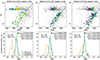 |
Fig. 1. Hertzsprung-Russell diagrams and mass distributions of Kepler high-α stars at three different metallicities. The [Fe/H] range and median in each panel is given at the top. Top panels: HR diagrams of the selected stars. The colour coding spans the metallicities in each bin with darker colours being more metal poor. Solid lines represent MESA models of the median [Fe/H], median [α/Fe], and median mass of each bin, shifted by −126 K, consistent with our analysis in Sect. 4.1. Bottom panels: The Kepler mass histograms based on asteroseismology from Yu et al. (2018) and Gaia DR3 parallax zero-points from Lindegren et al. (2021). The mass distributions of RGB and HeCB stars are calculated using Eq. (1), and for the RGB stars also using PARAM with Δν and νmax as input. The number of stars N and the median mass of each evolutionary phase are shown along with the mass loss, ΔM, the difference in median mass between the HeCB and RGB distributions. |
The average integrated mass loss is seen to increase with decreasing metallicity from 0.082 to 0.110 to 0.167 M⊙. This significant trend is also seen in Fig. 2 where we fit linear relations to the full metallicity range and find clearly different slopes for RGB and HeCB stars, respectively. The scatter around the fit to the RGB stars is consistent with measurement uncertainties only, as seen from the sizes of the median 1σ and maximum 1σ error bars of the individual stars. From the difference between the lines of the RGB and HeCB stars, we obtain
![Mathematical equation: $$ \begin{aligned} \Delta M/\mathrm M_{\odot } =(-0.216\pm 0.025) \times [\mathrm{Fe/H}] + (0.036\pm 0.010). \end{aligned} $$](/articles/aa/full_html/2024/11/aa52033-24/aa52033-24-eq2.gif) (2)
(2)
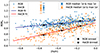 |
Fig. 2. Mass vs [Fe/H] for RGB and HeCB Kepler giants. Black binned data points correspond to the bins in Fig. 1. The lines represent linear fits to rolling medians. The blue and orange double error bars represent the median and maximum 1σ mass uncertainty of the RGB and HeCB stars, respectively. |
The trend is supported by our corresponding analysis of the K2 stars, although they show a shallower trend and at lower significance; see Appendix A.2. We thus find clear evidence that RGB mass loss increases with decreasing metallicity. As the RGB median mass is inversely correlated with metallicity, as expected for a nearly coeval population, the mass-loss trend could also be a trend with initial mass. More information is needed to establish whether it is metallicity or initial mass that is driving the trend, or indeed both.
4. Hertzsprung-Russell and colour–magnitude diagram mass loss from GCs
The RGB mass loss that we infer from asteroseismology is independent of stellar models. Here, we examine its compatibility with model predictions for metal-rich GCs in the HR diagram and CMD.
Globular clusters are known to host multiple populations (Gratton et al. 2012) where only the first generation (1G) is expected to have a helium content similar to that of field stars (Milone et al. 2018). We therefore compare HeCB stars from our asteroseismic samples to 1G GC HeCB stars with similar [Fe/H] and [α/Fe].
4.1. HR comparison to metal-rich HeCB GC stars
In Fig. 3 we compare the HR diagram positions of HeCB stars from our Kepler and K2 samples and two GCs with a metallicity of close to [Fe/H] = −0.50 as detailed in the legend of the top panel. In particular, the HeCB stars in NGC 6304 have [Fe/H], [α/Fe], and Teff measured by APOGEE DR17 (Schiavon et al. 2024), the same source we used for the Kepler and K2 stars. This is therefore a direct Teff comparison of HeCB stars in a GC and the field with the least possible amount of relative systematic error. Similarly, the chosen HeCB stars from NGC 6352 sample the colour extent of the 1G HeCB stars in this cluster well and have spectroscopic measurements (Feltzing et al. 2009), although not by APOGEE. For both GCs, luminosities were derived using the spectroscopic Teff and [Fe/H] values together with KS magnitudes (Skrutskie et al. 2006), reddening, and true distance moduli as derived below from CMD fitting and bolometric corrections (Casagrande & VandenBerg 2014) for KS.
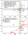 |
Fig. 3. Hertzsprung-Russell diagrams of α-rich HeCB stars in the Kepler and K2 fields compared to metal-rich GC HeCB stars and model predictions. Top panel: Kepler and K2 HeCB stars with −0.55 < [Fe/H] < − 0.45 compared to GC stars of similar metallicity. The median colour of HeCB stars in each GC is corrected to [Fe/H] = −0.50 based on model comparisons in the bottom panel. Bottom panel: MESA HeCB stellar model track and median locations of various masses and compositions compared to observed median values. All model Teff values are shifted by −126 K to reach agreement with the observed Kepler median Teff at the corresponding observed 0.8 M⊙. Crosses of different colours mark median locations of HeCB stars of different compositions. Model based translations between mass difference and temperature difference are illustrated by black double-arrows. Coloured double arrows mark the corresponding observed mass differences between the Kepler and GC HeCB medians. |
Directly comparing the GC stars to the field stars, their very similar effective temperatures suggest that their masses are also relatively similar. As there are many fewer GC stars and their individual uncertainties are larger, their mean Teff values can be affected by sampling and evolution effects. However, as seen in Fig. 4, the stars with spectroscopic Teff measurements sample the colour extent of the 1G HeCB stars well. Removing the most outlying star at either end changes the mean Teff from 4967 K by −11 or +8 K, and the median is 4950 K in all three cases. Resampling the Teff of nine randomly chosen stars from the entire sample of 1G photometric members from Fig. 4 1000 times results in a mean Teff of 4985 K with a maximum deviation of the median of less than 20 K. We made similar evaluations for NGC 6304, although these were less direct and were performed using Gaia photometry, as the stars with spectroscopy do not have HST photometry. Systematic errors in spectroscopic Teff estimates can typically be at a level of about 80 K (Bruntt et al. 2010). However, in our case, NGC 6304 was spectroscopically analysed with the exact same instrument and method as the field stars, which should minimise systematic uncertainties in comparisons.
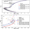 |
Fig. 4. Hubble Space Telescope CMDs of NGC 6352 with Victoria isochrones and ZAHBs and a MESA HeCB evolutionary track. Panel a: Full CMD. Parameters equal for all models are given in the top left corner. The black dashed arrow is the reddening vector. Panel b: Zoom onto the RHB. Squares and star symbols mark 1G and 2G stars, respectively. Stars with spectroscopic measurements are marked with squares, with purple corresponding to 4900 K, blue to 4950 K, green to 5000 K, and yellow to 5050 K. The F606W − F814W colours of the corresponding temperatures are marked with vertical lines at the top border. The lowest luminosity RHB star is marked and dashed lines extending from it are used to estimate the HeCB mass at their intersections with ZAHBs. The sloped dashed line is along the reddening vector. |
The observed variation between models of different masses, as indicated by black double-headed arrows in the bottom panel of Fig. 3, can be used to translate the observed Teff differences into estimates of the mass difference. We used stellar model tracks computed using MESA v117011 (Paxton et al. 2011, 2013, 2015, 2018, 2019) with inputs as described by Matteuzzi et al. (2023). The temperature scale of these models was found to be too high compared to the observations. There are several uncertainties in current stellar models that can cause such offsets (e.g. see Silva Aguirre et al. 2020). One common issue that could be at the root of these offsets is the adoption of mixing length theory (e.g. see Joyce & Tayar 2023) and the connected solar mixing length parameter calibration procedure, which itself is connected to the choice of surface boundary condition (Salaris et al. 2018). To mitigate such potential offsets to the best of our ability, all the model predictions in Fig. 3 are shifted by −126 K so that the median Teff of a 0.80 M⊙ HeCB model track agrees with the median observed Teff of the Kepler stars, which also have a median mass very close to 0.80 M⊙. While this procedure may not be accurate, it is encouraging that this Teff shift also results in good agreement with the observed median luminosity of the Kepler stars, which only improves if one considers that they have slightly higher-than-primordial helium content (as assumed in the models shown in red). Additionally, the model tracks in Fig. 1 show a good match to both RGB and HeCB stars in all three [Fe/H] bins with this same offset applied, even though it was determined at one specific metallicity.
The masses of the HeCB GC stars are found to be 0.03–0.07 M⊙ lower than the field stars when relying on the relative Teff–mass dependence of the shifted models. This is seen from the distances to the vertical coloured lines in the bottom panel of Fig. 3, which mark the mean Teff values of the clusters corrected to the median metallicity of the field stars, [Fe/H]= − 0.50. Accordingly, our earlier considerations regarding potential uncertainties on the median Teff GC values at a level of below 20 K suggest an uncertainty of less than 0.05 M⊙. We emphasise that this is a relative comparison between field and GC star masses, and that the models are only used to translate differences in Teff and composition into differences in mass.
Relying instead on the comparison of the median luminosity of the GC stars to that of the Kepler stars in the top panel of Fig. 3, we see that the HeCB median mass is −0.01 to 0.04 M⊙ lower than that of the Kepler stars, but this is much more uncertain, as there are few HeCB GC stars with spectroscopic measurements, and part of the luminosity difference could be due to evolution. If relying on the faintest CHeB star in each GC to avoid this, then the HeCB mass in the two clusters would instead be about 0.10 M⊙ lower than the Kepler median, serving as a maximum difference estimate. As the GCs are likely older than the field stars, a mass difference is also expected for the RGB stars, which would result in very similar RGB mass loss for the metal-rich GCs and the Kepler and K2 field stars. We investigate this in the following subsection.
4.2. RGB mass loss from GC CMDs
Figure 4 shows the HST F606W − F814W, F606W CMD of NGC 6352 from the final data release (Nardiello et al. 2018) of the HUGS survey (Piotto et al. 2015) over-plotted with isochrones and zero-age horizontal branches (ZAHBs) from the Victoria models (VandenBerg et al. 2014; VandenBerg 2024). HeCB stars were separated into 1G and 2G using the F275W − F336W versus F336W − F438W diagram as in Tailo et al. (2022).
The models were matched to the observations employing the same nine HeCB GC stars with spectroscopic Teff measurements used in Fig. 3; E(B − V) was first adjusted to obtain the best average agreement between the spectroscopic Teff values and the corresponding photometric ones from F606W − F814W and the calibration by Casagrande & VandenBerg (2014). Then, the apparent distance modulus and age were found from a model-match to the main sequence, turn-off, and early SGB.
We inferred the minimum HeCB mass by comparing the absolute magnitude of the least luminous 1G HeCB star (black diamond in panel b of Fig. 4) to ZAHB loci. This can be accomplished along the sloped dashed line, which represents the direction of both the reddening vector and a change in metallicity. Errors in metallicity, reddening, and/or differential reddening therefore shift stars or the ZAHBs along this line. However, because of potential systematic uncertainties caused by, for example, mixing length theory and surface boundary conditions, it is also likely that the ZAHB will be shifted horizontally. Such a shift is unlikely to be past the red ZAHB shown, unless there are errors in the relative temperature scale, as the corresponding isochrone is already at the cool red edge of the observed RGB (see panel a of Fig. 4). Thus, one either obtains a minimum HeCB mass of about 0.86, 0.82, or 0.78 M⊙ depending on the assumed composition from a horizontal match, or lower values of about 0.79, 0.75, or 0.72 M⊙ from matches along the reddening line. These HeCB mass estimates were subtracted from the corresponding low-luminosity RGB masses from the CMD-matched model close to the RGB bump in panel a of Fig. 4 to obtain the mass-loss predictions. This yielded estimates of the integrated RGB mass loss in the ranges 0.07–0.14, 0.08–0.15, and 0.11–0.17 M⊙ for the chosen compositions. As seen, the range is not strongly dependent on composition, because changes to the RGB mass partly compensate for the changes to the HeCB mass estimates. We adopt the range 0.11–0.17 M⊙, which corresponds to the metallicity [Fe/H] = −0.55 measured by Feltzing et al. (2009) and with a helium content of Y = 0.256. As we cannot know which end of the range to prefer, we take the middle value as our best estimate and the distance to the range ends as the uncertainty, obtaining ΔM = 0.14 ± 0.03 M⊙. In the Appendix, we repeat the procedure for NGC 6304 for which we obtain ΔM = 0.13 ± 0.04 M⊙. Thus, the mass loss in these GCs is very similar to that inferred from asteroseismology of field stars at similar metallicity.
5. Discussion, conclusions, and outlook
We provide novel empirical constraints on the integrated RGB mass loss, crucially closing the gap between GCs, field stars, and open clusters with asteroseismic constraints.
-
By comparing the median mass of RGB and HeCB stars in nearly mono-age mono-metallicity populations of giants in the MW high-[α/Fe] sequence, we find ΔM to increase with decreasing metallicity/mass.
-
Such an increase in ΔM extends to M4, where constraints from asteroseismology and CMDs agree (Tailo et al. 2022).
-
GCs were reported in the literature to have increasing ΔM (Tailo et al. 2020) towards higher metallicity. Our RGB mass-loss estimates for NGC 6352 and NGC 6304 ([Fe/H] ∼ −0.5) are significantly smaller than those of Tailo et al. (2020) and are in agreement with our asteroseismic findings for Kepler and K2 field stars at similar metallicities and masses, suggesting that the mechanism and efficiency of RGB mass loss is the same for field and GC stars.
-
Current RGB mass-loss laws are unable to match all the asteroseismic integrated mass-loss estimates using a single value for the free parameter η. Figure 5 demonstrates this for Reimers’ law in comparison to the estimates for α-rich field stars presented in this work, as well as the GC M4 and the open clusters M67 and NGC 6791. We find comparable issues for similar prescriptions (see also Fig. 4 in Catelan 2009).
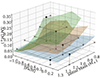 |
Fig. 5. Comparison of integrated mass-loss estimates from the GC M4 (Tailo et al. 2022), our most metal-poor and most metal-rich bins of α-rich field stars, and the open clusters M67 (Stello et al. 2016) and NGC 6791 (Miglio et al. 2012) to predictions from Reimers mass-loss law for different choices of η. Blue: η = 0.2, orange: η = 0.4, green: η = 0.6. |
The situation is further complicated by the fact that RGB mass-loss estimates in GCs suggest an increase in mass loss with increasing metallicity or mass, while our present findings suggest a decrease with increasing metallicity or mass. It might therefore be that the true mass-loss prescription is first increasing with increasing mass or metallicity at low metallicities, and that the trend reverses after some specific threshold. Further theoretical developments regarding the mechanism responsible for the mass-loss process on the RGB, combined with more precise asteroseismic measurements for additional GCs – which could be provided by a space mission like Haydn (Miglio et al. 2021b) – pave the way for transforming our understanding of mass loss from a rudimentary calibration to a well-defined physical insight.
MESA inlist is available on request.
Acknowledgments
We thank Don VandenBerg for providing Victoria isochrones and ZAHBs. This work has made use of data from the European Space Agency (ESA) mission Gaia (https://www.cosmos.esa.int/Gaia), processed by the Gaia Data Processing and Analysis Consortium (DPAC,https://www.cosmos.esa.int/web/Gaia/dpac/consortium). Funding for the DPAC has been provided by national institutions, in particular the institutions participating in the Gaia Multilateral Agreement. This paper includes data collected by the Kepler mission. Funding for the Kepler mission is provided by the NASA Science Mission directorate. Some of the data presented in this paper were obtained from the Mikulski Archive for Space Telescopes (MAST). STScI is operated by the Association of Universities for Research in Astronomy, Inc., under NASA contract NAS5-26555. Support for MAST for non-HST data is provided by the NASA Office of Space Science via grant NNX09AF08G and by other grants and contracts. Funding for the Stellar Astrophysics Centre was provided by The Danish National Research Foundation (Grant agreement no.: DNRF106). AM, EW, KB and WEvR acknowledge support from the ERC Consolidator Grant funding scheme (project ASTEROCHRONOMETRY, https://www.asterochronometry.eu, G.A. n. 772293).
References
- Abdurro’uf, Accetta, K., Aerts, C., et al. 2022, ApJS, 259, 35 [NASA ADS] [CrossRef] [Google Scholar]
- Anders, F., Chiappini, C., Rodrigues, T. S., et al. 2017, A&A, 597, A30 [NASA ADS] [CrossRef] [EDP Sciences] [Google Scholar]
- Bedding, T. R., Mosser, B., Huber, D., et al. 2011, Nature, 471, 608 [Google Scholar]
- Borucki, W. J., Koch, D., Basri, G., et al. 2010, Science, 327, 977 [Google Scholar]
- Brogaard, K., Arentoft, T., Miglio, A., et al. 2023, A&A, 679, A23 [NASA ADS] [CrossRef] [EDP Sciences] [Google Scholar]
- Bruntt, H., Bedding, T. R., Quirion, P. O., et al. 2010, MNRAS, 405, 1907 [Google Scholar]
- Casagrande, L., & VandenBerg, D. A. 2014, MNRAS, 444, 392 [Google Scholar]
- Casagrande, L., Silva Aguirre, V., Schlesinger, K. J., et al. 2016, MNRAS, 455, 987 [Google Scholar]
- Catelan, M. 2009, Ap&SS, 320, 261 [Google Scholar]
- da Silva, L., Girardi, L., Pasquini, L., et al. 2006, A&A, 458, 609 [NASA ADS] [CrossRef] [EDP Sciences] [Google Scholar]
- D’Antona, F., Caloi, V., Montalbán, J., Ventura, P., & Gratton, R. 2002, A&A, 395, 69 [CrossRef] [EDP Sciences] [Google Scholar]
- Elsworth, Y., Themeßl, N., Hekker, S., & Chaplin, W. 2020, Res. Notes Am. Astron. Soc., 4, 177 [Google Scholar]
- Feltzing, S., Primas, F., & Johnson, R. A. 2009, A&A, 493, 913 [NASA ADS] [CrossRef] [EDP Sciences] [Google Scholar]
- Gaia Collaboration (Vallenari, A., et al.) 2023, A&A, 674, A1 [NASA ADS] [CrossRef] [EDP Sciences] [Google Scholar]
- Gratton, R. G., Carretta, E., & Bragaglia, A. 2012, A&ARv, 20, 50 [CrossRef] [Google Scholar]
- Han, Z., Podsiadlowski, P., Maxted, P. F. L., Marsh, T. R., & Ivanova, N. 2002, MNRAS, 336, 449 [Google Scholar]
- Handberg, R., Brogaard, K., Miglio, A., et al. 2017, MNRAS, 472, 979 [CrossRef] [Google Scholar]
- Howell, S. B., Sobeck, C., Haas, M., et al. 2014, PASP, 126, 398 [Google Scholar]
- Howell, M., Campbell, S. W., Stello, D., & De Silva, G. M. 2022, MNRAS, 515, 3184 [NASA ADS] [CrossRef] [Google Scholar]
- Joyce, M., & Tayar, J. 2023, Galaxies, 11, 75 [NASA ADS] [CrossRef] [Google Scholar]
- Kallinger, T., Hekker, S., Mosser, B., et al. 2012, A&A, 541, A51 [NASA ADS] [CrossRef] [EDP Sciences] [Google Scholar]
- Khan, S., Miglio, A., Willett, E., et al. 2023, A&A, 677, A21 [NASA ADS] [CrossRef] [EDP Sciences] [Google Scholar]
- Li, Y., Bedding, T. R., Huber, D., et al. 2024, ApJ, 974, 77 [NASA ADS] [CrossRef] [Google Scholar]
- Lindegren, L., Bastian, U., Biermann, M., et al. 2021, A&A, 649, A4 [EDP Sciences] [Google Scholar]
- Matteuzzi, M., Montalbán, J., Miglio, A., et al. 2023, A&A, 671, A53 [NASA ADS] [CrossRef] [EDP Sciences] [Google Scholar]
- Miglio, A., Brogaard, K., Stello, D., et al. 2012, MNRAS, 419, 2077 [Google Scholar]
- Miglio, A., Chiappini, C., Mackereth, J. T., et al. 2021a, A&A, 645, A85 [NASA ADS] [CrossRef] [EDP Sciences] [Google Scholar]
- Miglio, A., Girardi, L., Grundahl, F., et al. 2021b, Exp. Astron., 51, 963 [NASA ADS] [CrossRef] [Google Scholar]
- Milone, A. P., Marino, A. F., Renzini, A., et al. 2018, MNRAS, 481, 5098 [NASA ADS] [CrossRef] [Google Scholar]
- Nardiello, D., Libralato, M., Piotto, G., et al. 2018, MNRAS, 481, 3382 [NASA ADS] [CrossRef] [Google Scholar]
- Paxton, B., Bildsten, L., Dotter, A., et al. 2011, ApJS, 192, 3 [Google Scholar]
- Paxton, B., Cantiello, M., Arras, P., et al. 2013, ApJS, 208, 4 [Google Scholar]
- Paxton, B., Marchant, P., Schwab, J., et al. 2015, ApJS, 220, 15 [Google Scholar]
- Paxton, B., Schwab, J., Bauer, E. B., et al. 2018, ApJS, 234, 34 [NASA ADS] [CrossRef] [Google Scholar]
- Paxton, B., Smolec, R., Schwab, J., et al. 2019, ApJS, 243, 10 [Google Scholar]
- Piotto, G., Milone, A. P., Bedin, L. R., et al. 2015, AJ, 149, 91 [Google Scholar]
- Reimers, D. 1975a, Mem. Soc. Roy. Sci. Liege, 8, 369 [Google Scholar]
- Reimers, D. 1975b, Problems in stellar atmospheres and envelopes, 229 [CrossRef] [Google Scholar]
- Rodrigues, T. S., Bossini, D., Miglio, A., et al. 2017, MNRAS, 467, 1433 [NASA ADS] [Google Scholar]
- Salaris, M., Cassisi, S., Schiavon, R. P., & Pietrinferni, A. 2018, A&A, 612, A68 [NASA ADS] [CrossRef] [EDP Sciences] [Google Scholar]
- Schiavon, R. P., Phillips, S. G., Myers, N., et al. 2024, MNRAS, 528, 1393 [CrossRef] [Google Scholar]
- Schröder, K. P., & Cuntz, M. 2005, ApJ, 630, L73 [CrossRef] [Google Scholar]
- Schröder, K. P., & Smith, R. C. 2008, MNRAS, 386, 155 [CrossRef] [Google Scholar]
- Silva Aguirre, V., Christensen-Dalsgaard, J., Cassisi, S., et al. 2020, A&A, 635, A164 [NASA ADS] [CrossRef] [EDP Sciences] [Google Scholar]
- Skrutskie, M. F., Cutri, R. M., Stiening, R., et al. 2006, AJ, 131, 1163 [NASA ADS] [CrossRef] [Google Scholar]
- Stello, D., Vanderburg, A., Casagrande, L., et al. 2016, ApJ, 832, 133 [NASA ADS] [CrossRef] [Google Scholar]
- Tailo, M., Milone, A. P., Lagioia, E. P., et al. 2020, MNRAS, 498, 5745 [CrossRef] [Google Scholar]
- Tailo, M., Corsaro, E., Miglio, A., et al. 2022, A&A, 662, L7 [NASA ADS] [CrossRef] [EDP Sciences] [Google Scholar]
- VandenBerg, D. A. 2024, MNRAS, 527, 6888 [Google Scholar]
- VandenBerg, D. A., Bergbusch, P. A., Ferguson, J. W., & Edvardsson, B. 2014, ApJ, 794, 72 [NASA ADS] [CrossRef] [Google Scholar]
- Yu, J., Huber, D., Bedding, T. R., et al. 2018, ApJS, 236, 42 [NASA ADS] [CrossRef] [Google Scholar]
Appendix A: Asteroseismic measurement details
In this section we provide details on our method to derive asteroseismic integrated mass-loss estimates.
As mentioned in the main text, we selected giants belonging to the α-rich population of the MW according to the selection criterion [α/Fe] > 0.1 − 0.8 ·[Fe/H], and split them into three [Fe/H] bins (see Figs. A.1– A.3). The bin ranges were chosen to obtain similar numbers of HeCB and RGB stars in each of the three bins for both the Kepler and K2 samples. RGB and HeCB stars were separated using different limits on νmax and Teff as detailed in Table A.1.
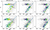 |
Fig. A.1. HR diagrams within the chosen metallicity bins for the Kepler and K2 samples with the quality cuts applied. |
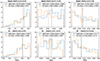 |
Fig. A.2. Histograms of metallicity distributions within the chosen metallicity bins for the Kepler and K2 samples with the quality cuts applied. Vertical dashed lines correspond to the median [Fe/H] of RGB and HeCB stars, respectively. |
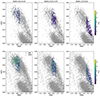 |
Fig. A.3. [α/Fe] vs [Fe/H] distributions of the selected stars. Grey dots are the full samples. Coloured circles and triangles indicate the selected RGB and HeCB stars. Colour-coating is according to Zmax, the distance from the MW disc plane. Top row are for Kepler stars, bottom row the K2 stars. |
Cuts & constraints for selection of stars
We then applied quality cuts as given in Table A.1. We removed stars with a νmax uncertainty above 5% and stars with an RGB mass from PARAM with an uncertainty above 7%. Constraints were also applied for the parallax and parallax uncertainty as explained below in Section A.2. The limits were chosen as a compromise between precision and the number of stars remaining in the bins. Additionally, cuts were made in the HR diagram to remove stars that appeared significantly hotter than the general RGB and fainter than the HeCB stars, since these are either stars whose parameters have been altered through binary evolution, or stars with bad measurements. Despite these cuts, few such over-massive stars remain in the samples, and we therefore also cut away stars more massive than the 95th percentile for each population separately. However, this did not alter significantly the values of the median masses or the integrated RGB mass loss.
The HR diagrams of our selected stars are shown in Fig. A.1. The Teff distributions of the RGB and HeCB stars cover similar ranges, minimising the possibility of the derived mass loss to be an artefact of systematics in the observed Teff scale, since the mass of RGB and HeCB would be affected in the same way. Although not shown, we also checked that there is no correlation between mass and luminosity for the RGB stars (but there is a correlation for HeCB which is expected from stellar evolution). Therefore, it is unlikely that systematic errors in luminosity between RGB and HeCB stars are biassing our mass-loss estimates.
Fig. A.2 shows histograms of the [Fe/H] distributions of RGB and HeCB stars in each metallicity bin to demonstrate that they are very similar. Differences in [Fe/H] medians and means between Kepler-K2 and RGB-HeCB are typically at or below 0.02 dex, sometimes as high as 0.03 dex. The general mass-change between panels suggest that a change of 0.01 dex in metallicity corresponds to a mass change of about 0.001 M⊙. Therefore, these small differences in metallicity have very limited influence on the derived masses and mass loss at the level of 0.002 M⊙.
For the Kepler sample, measurement uncertainties on νmax, Teff and luminosity are in general small enough that the inferences using the full sample did not change significantly even if various quality-cuts were tried. For the final results we decided for consistency reasons to anyway apply the same quality cuts as for the analysis of the K2 sample.
A.1. Kepler
Figure A.4 shows histograms of masses in the three metallicity-bins for RGB and HeCB stars, and values are given for the median mass and number of stars of each population in each bin along with ΔM, the integrated RGB mass loss, calculated as the difference between the median mass of RGB and HeCB stars, respectively. Uncertainties on the numbers are calculated by assuming Gaussian uncertainties and adding random uncertainties to each observable of each star before calculating the median mass 1000 times in a Monte Carlo run. For the RGB stars, there are two mass estimates; one based on νmax and luminosity using the Gaia parallax (Eq. 1), and another distance-independent estimate based on using both νmax and Δν in the Bayesian tool PARAM. The two mass estimates are close but do not agree within mutual 1σ uncertainties in two out of the three metallicity bins, reflecting that either uncertainties are slightly underestimated and/or are systematic in nature at this level. Among possible causes are small shifts to the parallax zero-points and/or the temperature scale. For stars in the RC we preferred not to use results from PARAM as they are found to be strongly dependent on the evolutionary tracks. The latter, by definition, occupy a rather small volume in the observables (L, Teff, νmax, ...) and any systematic difference between models and observations is found to have a strong impact on the mass estimates, which we would rather avoid in our study. In Fig. A.4 each set of three horizontal panels represent a different case. The top panels show the full sample of Kepler high-α stars without quality cuts and adopting asteroseismic parameters from Yu et al. (2018). The middle panel shows that no significant change occurs for the Kepler sample due to applying our quality cuts. The bottom panel adopts alternative asteroseismic measurements provided by Y. Elsworth (private comm.) calculated following Elsworth et al. (2020). This allows a more direct comparison to the K2 sample, which uses seismic values derived using that method.
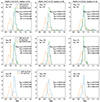 |
Fig. A.4. Mass distributions of stars in sub-samples of Kepler high-α stars at three different metallicities. The metallicity range and median metallicity in each panel is given above the top row. Each panel shows the mass distributions or RGB and RC stars separately, calculated using the scaling relation with νmax and luminosity, and for the RGB stars also the mass from PARAM with Δν and νmax as input. The number of stars the median mass values of each evolutionary phase are given. Also stated is the mass loss given as ΔM, the difference in mass between the RC and RGB phases. top panels: All stars in the sample. middle panels: With quality-cuts applied as described in the text. bottom panels: As middle panels, but using the average asteroseismic parameters from Elsworth et al. (2020) instead of Yu et al. (2018). |
A.2. K2
In Fig. A.4 we repeated the procedure for K2. Masses calculated from K2 data have significantly larger uncertainties because the time-series are much shorter and because the Gaia parallax zero-points are much more uncertain for the K2 fields than for the single Kepler field, even in a relative sense from one K2 field to another.
In the first two rows we employed a fixed -17 μas parallax zero-point correction with, and without, quality cuts applied, respectively. With this zero-point we found reasonable agreement between the RGB masses calculated from νmax plus luminosity from parallax and from PARAM using νmax and Δν. This was not the case when using the Lindegren et al. (2021) correction for the K2 fields, as can be seen in the fourth row. Note however that the same mass-loss trend remains despite this issue with the absolute masses.
To reduce potential problems from parallax zero-point errors we removed stars with  and
and  to avoid cases with large errors (> 5%) on parallax, either systematic or statistical. All but the top row panels of Fig. A.5 use these criteria.
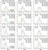 |
Fig. A.5. Similar to Fig. A.4 but for the K2 sample. 1. row: All stars in the sample. 2. row: With quality-cuts applied as described in the text and using a constant -17 μas parallax zero-point offset. 3. row: As 2. row, but using sector-based parallax zero-point offsets from Khan et al. (2023). 4. row: As 2. row, but using parallax zero-point offsets from Lindegren et al. (2021). |
Using a fixed parallax zero-point for all K2 fields is not necessarily correct, and (Khan et al. 2023) used a sample of 7024 K2 stars with asteroseismic and parallax information to infer zero-points for each field. We repeated our procedure while implementing these field-by-field parallax zero-points, which resulted in median mass changes at or below the 1 − σ level. These results are shown in the third row of panels in Fig. A.5.
The trend of the integrated mass loss for the K2 giants is similar to and consistent with that found for the Kepler giants, although the slope is shallower. However, as seen by comparing numbers in Fig. A.4 and Fig. A.5, the uncertainties are also larger, and the increase in mass loss between the metallicity bins depends on assumptions. To reach full 1σ agreement with the Kepler results, an uncertainty on the median masses larger than the statistical one needs to be adopted, at the level of 0.02 M⊙ for K2 and 0.01 M⊙ for Kepler. Thus, while the K2 result does support the Kepler result, it is less significant on its own.
Appendix B: RGB mass-loss dispersion
Fig. B.1 shows the observed Kepler mass distributions compared to simulations assuming the median mass represents stars with a single common mass at each [Fe/H] with the observed uncertainties from the real data. As seen, the distribution widths are compatible between observations and simulations for the RGB stars. For the HeCB stars, the simulations show narrower distributions than the observations unless additional scatter is applied. This additional scatter could arise due to underestimated uncertainties, but it could also be real. In the latter case, it could be interpreted as mass-loss dispersion since it is not present for the RGB stars. Two simulations are shown assuming a Gaussian mass-loss dispersion with σ of 0.05 and 0.08 M⊙, respectively. Due to the asymmetry of the observed distributions, it is difficult to interpret how to get a best match. A by-eye comparison of distribution widths suggests that 0.05σ is close to an upper limit and that 0.08 M⊙ is clearly too high.
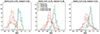 |
Fig. B.1. RGB mass-loss dispersion from observed Kepler vs. simulated mass histograms. |
Appendix C: GCs
In the main paper we used the CMD of the GC NGC 6352 to infer the integrated RGB mass loss by comparing to models.
We repeat here the procedure for NGC 6304 where we used [Fe/H] = −0.50 and [α/Fe]=+0.20, close to the values measured from APOGEE DR17 spectra by Schiavon et al. (2024), see Table C.1. Although they have a number of RHB stars in their sample, they are unfortunately not among the stars with HST photometry, so we cannot repeat the exact procedure from NGC 6352 to obtain the reddening estimate. Still, they are stars from the middle to the reddest part of the HB in the Teff range 4800-5000 K, which turn out to fall in the approximate photometric Teff range with the reddening that we adopt. The matching is shown in Fig. C.1. As can be seen from panel (b), the least luminous HeCB star depends on whether it is evaluated horizontally or along the reddening line. For this cluster, the separation between 1G and 2G populations is not clear, so we have not done that. However, the RHB stars at F606W − F814W = 0.7 and below are very likely 2G stars and therefore disregarded. Using the same procedure as for NGC 6352, we obtained a HeCB mass in the range 0.74-0.81 M⊙ resulting in a mass loss on the RGB of ΔM = 0.09 − 0.16 M⊙, similar to what we obtained for NGC 6352.
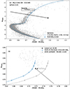 |
Fig. C.1. Colour-magnitude diagrams of NGC 6304 over-plotted with Victoria isochrones and ZAHBs. Similar to Fig. 4, but for NGC 6304. Panel a: Observed HST CMD compared to a model matched as described in the text. Model composition and RGB mass are given in the legend. Additional parameters are given in the top left corner. The reddening vector is shown as a black dashed arrow. Zoom box corresponding to panel (b) is marked. Panel b: Zoom on the HB. HB stars are marked with grey points. A ZAHB is over-plotted in blue with parameters as given in the legend, and the same ZAHB shifted in colour is shown in grey. The lowest luminosity HB star is marked with a diamond and lines extending from it are used to estimate the HB mass. The sloped dashed line is along the reddening vector. Note that depending on whether one shifts horizontally or along the reddening line, different stars are in this case the least luminous one. |
GC parameters
If the smallest HeCB star mass was instead deduced from colour while ignoring the absolute magnitude, it could be much different. However, that would then depend strongly on the exact reddening, differential reddening, assumptions on multiple populations and their helium contents, colour-temperature relations and the temperature scale of the models. Because of the unsolved model issues that can cause significant differences in model temperatures, for example the mixing length and surface boundary conditions, it is safer to rely on absolute magnitude instead of colour (or luminosity instead of effective temperature) to estimate the minimum HeCB mass from the CMD of metal-rich globular clusters, where HeCB stars of different masses are located much closer together in colour, and the mass-discrimination therefore becomes poorer.
All Tables
All Figures
|
Fig. 1. Hertzsprung-Russell diagrams and mass distributions of Kepler high-α stars at three different metallicities. The [Fe/H] range and median in each panel is given at the top. Top panels: HR diagrams of the selected stars. The colour coding spans the metallicities in each bin with darker colours being more metal poor. Solid lines represent MESA models of the median [Fe/H], median [α/Fe], and median mass of each bin, shifted by −126 K, consistent with our analysis in Sect. 4.1. Bottom panels: The Kepler mass histograms based on asteroseismology from Yu et al. (2018) and Gaia DR3 parallax zero-points from Lindegren et al. (2021). The mass distributions of RGB and HeCB stars are calculated using Eq. (1), and for the RGB stars also using PARAM with Δν and νmax as input. The number of stars N and the median mass of each evolutionary phase are shown along with the mass loss, ΔM, the difference in median mass between the HeCB and RGB distributions. |
| In the text | |
|
Fig. 2. Mass vs [Fe/H] for RGB and HeCB Kepler giants. Black binned data points correspond to the bins in Fig. 1. The lines represent linear fits to rolling medians. The blue and orange double error bars represent the median and maximum 1σ mass uncertainty of the RGB and HeCB stars, respectively. |
| In the text | |
|
Fig. 3. Hertzsprung-Russell diagrams of α-rich HeCB stars in the Kepler and K2 fields compared to metal-rich GC HeCB stars and model predictions. Top panel: Kepler and K2 HeCB stars with −0.55 < [Fe/H] < − 0.45 compared to GC stars of similar metallicity. The median colour of HeCB stars in each GC is corrected to [Fe/H] = −0.50 based on model comparisons in the bottom panel. Bottom panel: MESA HeCB stellar model track and median locations of various masses and compositions compared to observed median values. All model Teff values are shifted by −126 K to reach agreement with the observed Kepler median Teff at the corresponding observed 0.8 M⊙. Crosses of different colours mark median locations of HeCB stars of different compositions. Model based translations between mass difference and temperature difference are illustrated by black double-arrows. Coloured double arrows mark the corresponding observed mass differences between the Kepler and GC HeCB medians. |
| In the text | |
|
Fig. 4. Hubble Space Telescope CMDs of NGC 6352 with Victoria isochrones and ZAHBs and a MESA HeCB evolutionary track. Panel a: Full CMD. Parameters equal for all models are given in the top left corner. The black dashed arrow is the reddening vector. Panel b: Zoom onto the RHB. Squares and star symbols mark 1G and 2G stars, respectively. Stars with spectroscopic measurements are marked with squares, with purple corresponding to 4900 K, blue to 4950 K, green to 5000 K, and yellow to 5050 K. The F606W − F814W colours of the corresponding temperatures are marked with vertical lines at the top border. The lowest luminosity RHB star is marked and dashed lines extending from it are used to estimate the HeCB mass at their intersections with ZAHBs. The sloped dashed line is along the reddening vector. |
| In the text | |
|
Fig. 5. Comparison of integrated mass-loss estimates from the GC M4 (Tailo et al. 2022), our most metal-poor and most metal-rich bins of α-rich field stars, and the open clusters M67 (Stello et al. 2016) and NGC 6791 (Miglio et al. 2012) to predictions from Reimers mass-loss law for different choices of η. Blue: η = 0.2, orange: η = 0.4, green: η = 0.6. |
| In the text | |
|
Fig. A.1. HR diagrams within the chosen metallicity bins for the Kepler and K2 samples with the quality cuts applied. |
| In the text | |
|
Fig. A.2. Histograms of metallicity distributions within the chosen metallicity bins for the Kepler and K2 samples with the quality cuts applied. Vertical dashed lines correspond to the median [Fe/H] of RGB and HeCB stars, respectively. |
| In the text | |
|
Fig. A.3. [α/Fe] vs [Fe/H] distributions of the selected stars. Grey dots are the full samples. Coloured circles and triangles indicate the selected RGB and HeCB stars. Colour-coating is according to Zmax, the distance from the MW disc plane. Top row are for Kepler stars, bottom row the K2 stars. |
| In the text | |
|
Fig. A.4. Mass distributions of stars in sub-samples of Kepler high-α stars at three different metallicities. The metallicity range and median metallicity in each panel is given above the top row. Each panel shows the mass distributions or RGB and RC stars separately, calculated using the scaling relation with νmax and luminosity, and for the RGB stars also the mass from PARAM with Δν and νmax as input. The number of stars the median mass values of each evolutionary phase are given. Also stated is the mass loss given as ΔM, the difference in mass between the RC and RGB phases. top panels: All stars in the sample. middle panels: With quality-cuts applied as described in the text. bottom panels: As middle panels, but using the average asteroseismic parameters from Elsworth et al. (2020) instead of Yu et al. (2018). |
| In the text | |
|
Fig. A.5. Similar to Fig. A.4 but for the K2 sample. 1. row: All stars in the sample. 2. row: With quality-cuts applied as described in the text and using a constant -17 μas parallax zero-point offset. 3. row: As 2. row, but using sector-based parallax zero-point offsets from Khan et al. (2023). 4. row: As 2. row, but using parallax zero-point offsets from Lindegren et al. (2021). |
| In the text | |
|
Fig. B.1. RGB mass-loss dispersion from observed Kepler vs. simulated mass histograms. |
| In the text | |
|
Fig. C.1. Colour-magnitude diagrams of NGC 6304 over-plotted with Victoria isochrones and ZAHBs. Similar to Fig. 4, but for NGC 6304. Panel a: Observed HST CMD compared to a model matched as described in the text. Model composition and RGB mass are given in the legend. Additional parameters are given in the top left corner. The reddening vector is shown as a black dashed arrow. Zoom box corresponding to panel (b) is marked. Panel b: Zoom on the HB. HB stars are marked with grey points. A ZAHB is over-plotted in blue with parameters as given in the legend, and the same ZAHB shifted in colour is shown in grey. The lowest luminosity HB star is marked with a diamond and lines extending from it are used to estimate the HB mass. The sloped dashed line is along the reddening vector. Note that depending on whether one shifts horizontally or along the reddening line, different stars are in this case the least luminous one. |
| In the text | |
Current usage metrics show cumulative count of Article Views (full-text article views including HTML views, PDF and ePub downloads, according to the available data) and Abstracts Views on Vision4Press platform.
Data correspond to usage on the plateform after 2015. The current usage metrics is available 48-96 hours after online publication and is updated daily on week days.
Initial download of the metrics may take a while.