| Issue |
A&A
Volume 695, March 2025
|
|
|---|---|---|
| Article Number | A151 | |
| Number of page(s) | 7 | |
| Section | Extragalactic astronomy | |
| DOI | https://doi.org/10.1051/0004-6361/202451999 | |
| Published online | 14 March 2025 | |
Improving the accuracy of observable distributions for galaxies classified in the projected phase space diagram
1
Instituto de Astronomía Teórica y Experimental (CONICET – UNC), Laprida 854, X5000BGR Córdoba, Argentina
2
Observatorio Astronómico, Universidad Nacional de Córdoba, Laprida 854, X5000BGR Córdoba, Argentina
3
Departamento de Física Teórica, Universidad Autónoma de Madrid, 28049 Madrid, Spain
4
Instituto de Física Teórica, IFT-UAM/CSIC, C/ Nicolás Cabrera 13-15, Universidad Autónoma de Madrid, Cantoblanco, Madrid 28049, Spain
5
SISSA – International School for Advanced Studies, Via Bonomea 265, 34136 Trieste, Italy
6
Instituto de Astrofísica de La Plata (CONICET – UNLP), Observatorio Astronómico, Paseo del Bosque S/N, B1900FWA La Plata, Argentina
7
Facultad de Ciencias Astronómicas y Geofísicas, Universidad Nacional de La Plata, Observatorio Astronómico, Paseo del Bosque S/N, B1900FWA La Plata, Argentina
8
Facultad de Ingeniería y Arquitectura, Universidad Central de Chile, Av. Francisco de Aguirre 0405, La Serena, Chile
⋆ Corresponding author; This email address is being protected from spambots. You need JavaScript enabled to view it.
Received:
26
August
2024
Accepted:
5
February
2025
Abstract
Context. Studies of galaxy populations classified according to their kinematic behaviours and dynamical state using the projected phase space diagram (PPSD) are affected by misclassification and contamination, leading to systematic errors in determining the characteristics of the different galaxy classes.
Aims. We propose a method for statistically correcting the determination of galaxy properties’ distributions that accounts for the contamination caused by misclassified galaxies from other classes.
Methods. Using a sample of massive clusters and the galaxies in their surroundings taken from the MULTIDARK PLANCK 2 simulation combined with the semi-analytic model of galaxy formation SAG, we computed the confusion matrix associated with a classification scheme in the PPSD. Based on positions in the PPSD, galaxies are classified as cluster members, backsplash galaxies, recent infallers, infalling galaxies, or interlopers. This classification is determined using probabilities calculated by the code ROGER along with a threshold criterion. By inverting the confusion matrix, we are able to get better determinations of distributions of galaxy properties, such as colour.
Results. Compared to a direct estimation based solely on the predicted galaxy classes, our method provides better estimates of the mass-dependent colour distribution for the galaxy classes most affected by misclassification: cluster members, backsplash galaxies, and recent infallers. We applied the method to a sample of observed X-ray clusters and galaxies.
Conclusions. Our method can be applied to any classification of galaxies in the PPSD, and to any other galaxy property besides colour, provided an estimation of the confusion matrix is available. Blue, low-mass galaxies in clusters are almost exclusively recent infaller galaxies that have not yet been quenched by the environmental action of the cluster. Backsplash galaxies are on average redder than expected.
Key words: galaxies: clusters: general / galaxies: fundamental parameters / galaxies: statistics
© The Authors 2025
 Open Access article, published by EDP Sciences, under the terms of the Creative Commons Attribution License (https://creativecommons.org/licenses/by/4.0), which permits unrestricted use, distribution, and reproduction in any medium, provided the original work is properly cited.
This article is published in open access under the Subscribe to Open model. This email address is being protected from spambots. You need JavaScript enabled to view it. to support open access publication.
1. Introduction
In recent years, the projected phase space diagram (PPSD) has increasingly been used as a tool for classifying galaxies according to their kinematic behaviours and dynamical state in and around systems of galaxies, such as clusters and groups. The PPSD is a 2D space that combines the projected cluster-centric (or group-centric) distance with the line-of-sight velocity relative to the cluster (or group). Several authors have utilised the PPSD to study the evolution of galaxies. For example, Mahajan et al. (2011) studied the decrease in the star formation of backsplash galaxies (BSs). Muzzin et al. (2014) focused on the quenching of galaxies at z ∼ 1. Muriel & Coenda (2014) investigated the properties of high- and low-velocity galaxies in the outskirts of galaxy clusters. Hernández-Fernández et al. (2014) and Jaffé et al. (2015) studied the gas fraction and ram pressure of galaxies in clusters. Oman & Hudson (2016) studied the relationship between the star formation rates of a sample of observed galaxies and their likely orbital histories. Smith et al. (2019) analysed the stellar mass growth histories of galaxies as a function of their infall time. Martínez et al. (2023) studied the quenching of galaxies in a sample of X-ray clusters. Aguerri et al. (2023) focused on the properties of barred galaxies and their environments. Sampaio et al. (2024) examined the evolution of blue cloud, green valley, and red-sequence fractions as a function of time since infall. Muñoz Rodríguez et al. (2024) studied the impact on black hole growth as a function of the environment.
The aforementioned studies classify galaxies in systems and their outskirts following methods such as those proposed by Rhee et al. (2017), Pasquali et al. (2019), or de los Rios et al. (2021). Based on cosmological hydrodynamic N-body simulations of groups and clusters (Choi & Yi 2017), Rhee et al. (2017) categorised galaxies within the PPSD based on the time since their infall into the system. This categorisation included galaxies identified as first, recent, intermediate, and ancient infallers. They delineated specific regions within the PPSD where each of these types of galaxies are preferentially located. Pasquali et al. (2019) present an alternative approach that uses the same cosmological simulations (Choi & Yi 2017) of groups and clusters employed by Rhee et al. (2017). They established eight zones of constant mean infall time to investigate environmental influences on satellite galaxies. These zones are defined by analytical curves that characterise the timing of galaxy infall into the system.
Recently, de los Rios et al. (2021) presented the code ROGER1, which employs three different machine learning techniques to classify galaxies based on their projected phase-space positions within and around clusters. They utilised a dataset comprising massive and isolated galaxy clusters from the MULTIDARK PLANCK 2 simulation (Klypin et al. 2016). This code establishes a connection between the 2D phase space position of galaxies and their 3D orbital classifications. ROGER calculates the probabilities of galaxies belonging to any of the five orbital classes: cluster members (CLs), BSs, recent infallers (RINs), infallers (INs), and interlopers (ITLs).
Regardless of the chosen method for classifying galaxies in the PPSD, there will inevitably be some degree of contamination among the classes, particularly in regions closer to the centres of clusters. According to Coenda et al. (2022), misclassifications have significant implications for interpreting the properties of galaxies in the 2D classes. Therefore, the degree of contamination significantly impacts the conclusions that can be drawn. They emphasise the importance of distinguishing between red and blue galaxy populations to achieve a more precise analysis of observational data. Furthermore, they argue that the 2D analysis reliably provides results only for RINs, INs, and ITLs within the blue population.
To improve determinations of distributions of galaxy observables, such as colours or the specific star formation rate, for galaxies that have been classified using their position in the PPSD, we propose a simple method that reconstructs the intrinsic distribution of galaxy properties. The method relies on a statistic estimation of how well the classification is performed. This paper is organised as follows: In Sect. 2 we present our method; in Sect. 3 we test the method on a sample of simulated clusters and galaxies; in Sect. 4 we use the method to reconstruct the distributions of colours of galaxies of different classes in and around a sample of X-ray clusters of galaxies; finally, we present our conclusions and mention possible further uses of the method in Sect. 5.
2. Method
If we consider n classes of galaxies according to the particular classification scheme based on the PPSD we are using, the intrinsic class of each galaxy cannot be determined based solely on its position on it. At best, we can assign a particular class to a galaxy based on its position in the PPSD using our chosen methodology. In our case, this involves utilising the output probabilities of ROGER combined with a numerical criterion on their values, as we explain in Sect. 3. This way, each galaxy is assigned a predicted class. Due to uncertainties inherent to the classification procedure, the number of galaxies in the i-th predicted class (i = 1, …, n), NiP, is built up from the contribution of galaxies, in principle from all intrinsic classes, that were classified as class i:
 (1)
(1)
where NjI is the number of galaxies in our sample that belong to the j-th intrinsic class, and Cij is the fraction of galaxies of the j-th intrinsic class that were classified as being part of the i-th predicted class. The ideal case is Cij = δij, that is, a Kronecker delta. The quantities Cij are the elements of the confusion matrix, C, which has dimensions n × n.
The primary drawback of imperfect classification arises when studying the characteristics of galaxy populations using predicted classes, a method extensively used in the literature. Without any knowledge of C, results from such studies can be misleading. If we want to determine the distribution of a particular galaxy property, x (e.g. colour, specific star formation rate, size, etc.) for galaxies of a given stellar mass or, alternatively, absolute magnitude (M), the observed distributions of the property, x, are obtained by counting galaxies of a predicted class in m bins of x at a fixed M. The fraction of galaxies of the i-th predicted class with xk − Δxk/2 ≤ x ≤ xk + Δxk/2 and normalised to have unity area when integrating over the whole range of x is
 (2)
(2)
where the intrinsic (desired) quantities are the Fjk(M). The normalisation condition is
 (3)
(3)
There is no need for the bins in x to have equal size as long as we use the same binning for all classes.
If we have an estimation of C, for instance, by using numerical simulations, we can use Eq. (2) to solve for Fjk(M). By arranging the quantities fik(M) in a n × m matrix, f, with rows i (classes) and columns k (bins in x), and doing the same for Fjk(M) in F, now Eq. (2) reads
 (4)
(4)
Assuming det(C)≠0, the desired distributions are obtained as the rows of the n × m matrix:
 (5)
(5)
It is important to remark that so far we have assumed that the confusion matrix does not depend on mass (or absolute magnitude). In Sect. 3.3 we explore whether a stellar mass dependence of the confusion matrix (i.e. C ≡ C(M)) provides better results.
In the next section, we test the reliability of our method on a sample of simulated massive clusters of galaxies.
3. Application to a simulated sample of clusters of galaxies
3.1. The sample of simulated clusters and galaxies
We used the same sample of clusters and galaxies used by de los Rios et al. (2021) to train and test the code ROGER. The sample of cluster includes 34 massive systems, M200 ≥ 1015 h−1 M⊙, from the MULTIDARK PLANCK 2 simulation (Klypin et al. 2016). These clusters were selected to ensure that they do not have a companion halo more massive than 10% of M200 within 5 × R200. The mass M200 is estimated by considering an homogeneous mass distribution enclosed by a characteristic radius of a dark matter halo, R200, at which the density is equal to 200 times the critical density of the Universe at the redshift of the system.
The sample of galaxies in these clusters, and in their surroundings, were modelled by means of the semi-analytic model of galaxy formation SAG (Cora et al. 2018). The sample of simulated galaxies used in de los Rios et al. (2021) includes all SAG-MDPL2 galaxies at z = 0 with stellar mass greater than 108.5 h−1 M⊙ located within cylindrical volumes centred in the clusters with radius 3 × R200, and an extension along the simulated box’s z-axis of ±3σ in velocity (Hubble’s plus peculiar), where σ is the line-of-sight velocity dispersion of the galaxies in the cluster alongside the box’s z-axis.
Galaxies within these volumes were classified into five intrinsic classes according to their past orbits around the clusters (see de los Rios et al. 2021, for more details):
-
Cluster members: They may have crossed R200 several times in the past and are now found orbiting around the cluster centre, with the majority of them within R200 of the centre.
-
Backsplash galaxies: Galaxies that have crossed twice R200. The first time diving in, and the second time on their way out of the cluster, where they are now. Most of them will fall back into the cluster in the future.
-
Recent infallers: Galaxies that have crossed R200 only once as they dived into the cluster in the past 2 Gyr. Many of them may be BS in the future.
-
Infalling galaxies: Galaxies that have always been at distances greater than R200 from the cluster centre, and have negative radial velocity relative to the cluster. These galaxies are falling to the cluster.
-
Interlopers: Galaxies that have never gotten closer than R200 from the cluster centre but, unlike INs, have positive radial velocities relative to the cluster, that is, they are receding away from the cluster at z = 0. We consider these galaxies as objects that will not fall into the cluster. They are unrelated to the cluster but can be confused with classes 1−4 above in the PPSD (i.e. they are contamination).
Of the total of 30 289 galaxies, we used half of them to re-train ROGER (the training set), and the other half is the test set, which is the subsample of galaxies we used to compute the confusion matrix C. In de los Rios et al. (2021), we used ∼80% of the complete sample as training set, and the remaining as the test set. Here, we are interested in having a larger test set; thus, for the sake of consistency, we re-trained ROGER accordingly. It is noteworthy that we used a PYTHON version of ROGER, which we dub PYROGER, that is publicly available at ROGER’s website.
For each galaxy in the test set, we used PYROGER to compute its probability of being a member of each class, pi where i = 1, …, 5, and the correspondence between index and class is as listed above: 1 ↔ CL, 2 ↔ BS, 3 ↔ RIN, 4 ↔ IN, and 5 ↔ ITL. ROGER computes these probabilities using three different techniques: K-nearest neighbours, support vector machine, and random forest. We refer the reader to de los Rios et al. (2021) for details. For the purposes of this work, we used the probabilities that PYROGER computes using the K-nearest neighbours technique.
We used the classification scheme adopted by Coenda et al. (2022): the predicted class is defined by the highest value of pi, and this value has to be higher than a class-dependent threshold. These thresholds are 0.4, 0.48, 0.37, 0.54, and 0.15, for CLs, BSs, RINs, INs, and ITLs, respectively. This scheme is an appropriate balance between sensitivity and precision.
3.2. Applying the method
As a first step, we constructed the confusion matrix using the test set and computed Cij, the fraction of galaxies of predicted class i that are intrinsically of class j. For a better visualisation, instead of simply providing the numbers, we show the confusion matrix in Fig. 1. We can see in Fig. 1 how the predicted classes are composed in terms of the real classes. Predicted ITLs are the simplest case; they are basically real ITLs with a mild contamination (13%) of INs. Predicted INs are roughly real INs with two sources of contamination: 30% ITLs and 9% BSs. As for the predicted RINs, 52% are real RINs, with an unsurprising main source of contamination from CLs (23%) and lower (≤10%) percentages from the other classes. Of the predicted BSs, 53% are real BSs, and their main contamination comes from misclassified INs (32%). Finally, only 44% of the predicted CLs are real CLs; their most significant contamination is from RINs (26%), and in second place BSs and INs contributing ∼10% each. We refer the reader to de los Rios et al. (2021) for a thorough discussion on how the contamination between the five classes works. The three most contaminated predicted classes, CLs, BSs, and INs, are the most interesting ones for studying the effects of environments in the evolution of galaxies.
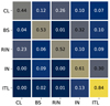 |
Fig. 1. Confusion matrix for our adopted classification scheme (Coenda et al. 2022). Columns correspond to intrinsic classes, rows to predicted classes. |
In Fig. 2 we present the distributions of x = u − r colour for the intrinsic classes, the predicted classes, and the reconstructed distributions obtained through the inversion of the confusion matrix, according to the adopted classification scheme. We split galaxies into five stellar mass bins in our analysis. To quantify whether our method provides better estimations of the intrinsic colour distribution, we computed the sum of squared residuals for each class i. This was done by comparing the intrinsic distributions (Fik(M), where k = 1, …, m denote the bins in colour) with the colour distributions of both the predicted classes (fik(M)) and the distributions recovered by our method,  :
:
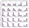 |
Fig. 2. Colour distributions of galaxies. Each class is shown in a different row, as noted to the right of the panels. Each column considers a particular range of galaxy stellar mass, as noted at the top. Grey shaded histograms are the real colour distributions, i.e. they correspond to the intrinsic classes. Green lines are the colour distributions of the predicted classes. Violet lines are the colour distributions recovered by our method. We quote within each panel the values of the corresponding square residuals, Spred and Srec, given by Eqs. (6) and (7), respectively. |
![Mathematical equation: $$ \begin{aligned} {S}_i^\mathrm{pred}(M)=\sum _{k=1}^m\Big [f_{ik}(M)-F_{ik}(M)\Big ]^2, \end{aligned} $$](/articles/aa/full_html/2025/03/aa51999-24/aa51999-24-eq7.gif) (6)
(6)
and
![Mathematical equation: $$ \begin{aligned} {S}_i^\mathrm{rec}(M)=\sum _{k=1}^m\Big [F_{ik}^\mathrm{rec}(M)-F_{ik}(M)\Big ]^2. \end{aligned} $$](/articles/aa/full_html/2025/03/aa51999-24/aa51999-24-eq8.gif) (7)
(7)
We note that we computed the square residuals and not χ2 since there are bins where Fik(M) = 0. These quantities are quoted inside each panel in Fig. 2. For a better visualisation and comparison, we show in Fig. 3 the sum of square residuals as a function of stellar mass. We note that y-axis scale varies from panel to panel in Fig. 3.
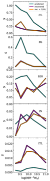 |
Fig. 3. Sum of square residuals as a function of galaxy stellar mass. Each panel considers a different galaxy class. Residuals between the real and the predicted distributions are shown with green lines, i.e. Spred in Eq. (6). Residuals between the real and the recovered distributions are shown with violet lines, i.e. Srec in Eq. (7). The residuals between the real and the recovered distributions when we use a stellar mass-dependent confusion matrix are shown in orange. Note that the y-axis scale varies from panel to panel. |
A joint analysis of Figs. 2 and 3 gives two general conclusions: on the one hand, our method improves the determination of the colour distribution of the three predicted classes that are more affected by misclassifications, namely, CLs, BSs, and RINs; and on the other hand, it does not improve the results for INs and ITLs, which are the two predicted classes best classified by our adopted criteria. These two main results are promising for this type of study; however, there is more to consider beyond just two levels of contamination, namely high contamination for CLs, BSs, and RINs and low contamination for INs and ITLs. Regarding their intrinsic colour distributions, the IN and ITL classes are the most similar, while the other three classes show greater variations from one to another. This is the consequence of very different evolutionary paths. Delving into the specifics, there are several interesting details in Figs. 2 and 3, which we summarise below.
-
Cluster members: Our method improves greatly the determination of the colour distributions in all five stellar mass bins. The predicted CL class exhibits a contamination from blue galaxies, which is particularly strong in the lower-mass bins. These galaxies are mostly RINs, and in a second place BSs, incorrectly classified as CLs. Distributions recovered by our method eliminate most of this contamination. We consistently find
 for all mass bins.
 -
Backsplash galaxies: As in the previous case, there are clear improvements for BS galaxies too, consisting in the removal of the contamination from blue, and mainly INs, galaxies. For all mass bins we find
 . Backsplash galaxies are, on average, redder when contamination effects are removed by our method.
 -
Recent infallers: With the exception of the highest-mass bin, we find that the method produces better results (i.e.
 . The improvement is most notably seen in the removal of the contamination from misclassified red CL galaxies with stellar mass in the range 9.7 ≤ log(M/h−1 M⊙)≤10.5 (see the third and fourth columns in Fig. 2). Our findings for CLs above and for RINs here suggest that almost every blue galaxy found in a cluster should have dived in there recently. This could have implications on the characterisation of satellites in clusters according to their dynamical state (e.g. Aldás et al. 2023, 2024).
 -
Infalling galaxies: In this case the method gives results comparable to the raw predictions. We can observe no significant differences between the intrinsic, the predicted, and the recovered distributions in Fig. 3. The values of the sum of square residuals are
 for three alternate mass bins, and otherwise in the remaining two. We note that
  and
and  are very similar in all cases and take values ∼1 − 2 × 10⁻², which is, on average, smaller than the corresponding values we find for CLs, BSs, and RINs.
 -
Interlopers: As said before, for this class, our method provides no improvement at all, but this should not be considered as a problem since there are virtually no differences between the intrinsic, predicted and recovered colour distributions, as in the previous case. In all five mass bins we obtain
 , but we note that all numerical values (∼10−3) are an order of magnitude smaller than for INs.
3.3. The effects of a mass dependence of matrix C
We explored the effect on our method of a possible dependence of the confusion matrix on the mass of galaxies. For each mass bin considered in Fig. 2, we computed a confusion matrix, C(M), using only those galaxies in the test sample that have stellar mass in the bin. The matrices so obtained (not shown here) do have a mild dependence on mass. However, this dependence do not change the results discussed in the previous subsection in a significant way. In Fig. 3, we present the resulting values of Sirec(M) as orange lines, where it is evident that the differences compared to the case of a unique C are really small. We can safely affirm there is no need to use a mass-dependent (or absolute-magnitude-dependent) confusion matrix. Furthermore, a mass-dependent confusion matrix implies a greater dependence on the specifics of how the galaxy evolution model works. It is desirable to minimise reliance on the model as much as possible.
The confusion matrix may depend on multiple parameters involved in the classification procedure, not just the stellar mass of the galaxies. In our particular case, classification was performed using specific thresholds on the probabilities computed by our code ROGER, which was trained on massive clusters from a specific cosmological simulation combined with a particular semi-analytic model. It is clear that the confusion matrix depends not only on these thresholds but also on the choices made during the training process. Given the nature of the input data used for classification, namely, the position in the PPSD, we do not expect the specific details of the semi-analytic model to have a significant impact on the confusion matrix. However, the choice of the mass range of the clusters used to train ROGER is likely to have a considerable effect. Other factors may also play a role, such as the degree of relaxation of the clusters. Assessing the influence of these various factors on the confusion matrix would require a comprehensive study that is beyond the scope of this paper. Nevertheless, the key aspect of the method proposed in this paper lies in constructing a confusion matrix that best represents the specifics of the classification performed. Achieving this will most likely require the use of numerical simulations of the galaxy systems under study.
4. Application to an observed sample of X-ray clusters of galaxies
As an example of the potential of the proposed statistical technique to correct the effects of misclassification, we applied our method to the sample of X-ray clusters and Sloan Digital Sky Survey (SDSS) galaxies used in Martínez et al. (2023). The sample comprises 104 X-ray clusters drawn from the works by Coenda & Muriel (2009) and Muriel & Coenda (2014), where the authors compute a number of properties of clusters originally catalogued by Popesso et al. (2004) and Bohringer et al. (2000), respectively. Martínez et al. (2023) searched for all spectroscopic SDSS-DR7 (Abazajian et al. 2009) galaxies within cylindrical volumes in redshift space centred in the clusters, and with radius 3 × R200 in projection and a longitude of ±3 × σ alongside the line-of-sight of the cluster. Galaxies were classified in the five classes under study using their positions in the PPSD, the ROGER-computed probabilities, and the thresholds of Coenda et al. (2022).
Using the confusion matrix computed in Sect. 3.2, we estimated the predicted and recovered distributions of the 0.1(u − r) colour of the five classes in four bins in stellar mass. The resulting distributions are shown in Fig. A.1. The outcome of applying our method to this sample of observed galaxies and clusters qualitatively agrees with our findings in Sect. 3.2, which were derived from applying the method to a simulated galaxy catalogue. We can observe basically the same trends of Fig. 3. For CL, the distributions recovered by our method eliminate most of the contribution from blue galaxies, this is more notorious in the lower-mass bins. According to the insights of Sect. 3.2, these blue galaxies are mostly actual RINs. In the case of BSs, the main feature we obtain is the removal of the contamination from blue galaxies, particularly at the lowest-mass bin. According to the confusion matrix we used (see Sect. 3.2), some 70% of the contamination should be due to galaxies erroneously classified as INs. Regarding RINs, the result of our method is most notably seen in the removal of a population of red, almost exclusively CLs, most clearly in the lower-mass bins. As in Sect. 3.2, for INs, the method gives results very similar to the raw predictions. Finally, for ITLs, once again, there are virtually no differences between the predicted and recovered colour distributions.
5. Conclusions
We propose a method for recovering the distributions of observed properties of galaxies classified according to their position in the PPSD. The method requires knowledge of the confusion matrix, or at least an estimation of it, which is inverted and applied to observed distributions. We tested this method on simulated clusters and galaxies and applied it to a sample of galaxies and X-ray clusters from the SDSS. For both simulated and observed galaxies, we classified galaxies in the PPSD using the code ROGER from de los Rios et al. (2021) plus the criteria from Coenda et al. (2022). In particular, we utilised colour as the parameter for analysing the distributions. These two choices, namely (i) the classification using ROGER plus thresholds and (ii) colour, are not essential to our objectives. Any classification scheme over the PPSD, such as those by Rhee et al. (2017) and Pasquali et al. (2019), and any galaxy property would be suitable provided one has an estimation of the confusion matrix.
Using the inversion of the confusion matrix along with our ROGER-based classification provides a better estimation of the distribution of colours of galaxies in and around clusters. The method is successful at decontaminating different classes of galaxies from the contamination of other classes, and it is particularly useful for regions of the PPSD where the overlap between classes complicates the classification most. The proposed method enables further analyses of galaxies when the classification is an issue. It is straightforward to reconstruct some statistics of galaxy populations as a function of stellar mass (or absolute magnitude). For instance, from Fig. A.1, we can compute the median of the colour distribution as a function of mass for the blue and red galaxy populations of each galaxy class.
We can draw some conclusions from the results we obtain for the five classes. The bulk of galaxies in clusters that are blue and less massive than M ≃ 1010.5 h−1 M⊙ are RINs. In terms of colour, BSs are on average in between CLs and RINs, while being distinctly redder than INs. Thus, a single excursion through the inner regions of a cluster produces significant changes in galaxy colour, due to a quench in star formation (e.g. Hough et al. 2023; Ruiz et al. 2023).
It is crucial to emphasise that analysing the properties of galaxies in systems derived directly from orbits obtained through phase space can lead to erroneous conclusions due to contamination effects between different classes. Therefore, the implementation of techniques aimed at minimising these biases, such as the one presented in this work, is highly important.
Acknowledgments
This paper has been partially supported with grants from Consejo Nacional de Investigaciones Científicas y Técnicas (PIPs 11220130100365CO, 11220210100064CO, 11220200102832CO and 11220200102876CO), Argentina, the Agencia Nacional de Promoción Científica y Tecnológica (PICTs 2018-3743, 2020-3690 and 2021-I-A-00700), Argentina, Secretaría de Ciencia y Tecnología, Universidad Nacional de Córdoba, Argentina, and Universidad Nacional de La Plata (G11-183), Argentina. MdlR acknowledges financial support from the Comunidad Autónoma de Madrid through the grant SI2/PBG/2020-00005. MdlR is supported by the Next Generation EU program, in the context of the National Recovery and Resilience Plan, Investment PE1 – Project FAIR “Future Artificial Intelligence Research”. The COSMOSIM database used in this paper is a service by the Leibniz-Institute for Astrophysics Potsdam (AIP). The MULTIDARK database was developed in cooperation with the Spanish MultiDark Consolider Project CSD2009-00064. The authors gratefully acknowledge the Gauss Centre for Supercomputing e.V. (www.gauss-centre.eu) and the Partnership for Advanced Supercomputing in Europe (PRACE, www.prace-ri.eu) for funding the MULTIDARK simulation project by providing computing time on the GCS Supercomputer SuperMUC at Leibniz Supercomputing Centre (www.lrz.de).
References
- Abazajian, K. N., Adelman-McCarthy, J. K., Agüeros, M. A., et al. 2009, ApJS, 182, 543 [Google Scholar]
- Aguerri, J. A. L., Cuomo, V., Rojas-Roncero, A., & Morelli, L. 2023, A&A, 679, A5 [NASA ADS] [CrossRef] [EDP Sciences] [Google Scholar]
- Aldás, F., Zenteno, A., Gómez, F. A., et al. 2023, MNRAS, 525, 1769 [CrossRef] [Google Scholar]
- Aldás, F., Gómez, F. A., Vega-Martínez, C., Zenteno, A., & Carrasco, E. R. 2024, ArXiv e-prints [arXiv:2408.05305] [Google Scholar]
- Bohringer, H., Voges, W., Huchra, J. P., et al. 2000, VizieR Online Data Catalog: J/ApJS/129/435 [Google Scholar]
- Choi, H., & Yi, S. K. 2017, ApJ, 837, 68 [NASA ADS] [CrossRef] [Google Scholar]
- Coenda, V., & Muriel, H. 2009, A&A, 504, 347 [NASA ADS] [CrossRef] [EDP Sciences] [Google Scholar]
- Coenda, V., de los Rios, M., Muriel, H., et al. 2022, MNRAS, 510, 1934 [Google Scholar]
- Cora, S. A., Vega-Martínez, C. A., Hough, T., et al. 2018, MNRAS, 479, 2 [Google Scholar]
- de los Rios, M., Martínez, H. J., Coenda, V., et al. 2021, MNRAS, 500, 1784 [Google Scholar]
- Hernández-Fernández, J. D., Haines, C. P., Diaferio, A., et al. 2014, MNRAS, 438, 2186 [CrossRef] [Google Scholar]
- Hough, T., Cora, S. A., Haggar, R., et al. 2023, MNRAS, 518, 2398 [Google Scholar]
- Jaffé, Y. L., Smith, R., Candlish, G. N., et al. 2015, MNRAS, 448, 1715 [Google Scholar]
- Klypin, A., Yepes, G., Gottlöber, S., Prada, F., & Heß, S. 2016, MNRAS, 457, 4340 [Google Scholar]
- Mahajan, S., Mamon, G. A., & Raychaudhury, S. 2011, MNRAS, 416, 2882 [NASA ADS] [CrossRef] [Google Scholar]
- Martínez, H. J., Coenda, V., Muriel, H., de los Rios, M., & Ruiz, A. N. 2023, MNRAS, 519, 4360 [CrossRef] [Google Scholar]
- Muñoz Rodríguez, I., Georgakakis, A., Shankar, F., et al. 2024, MNRAS, 532, 336 [CrossRef] [Google Scholar]
- Muriel, H., & Coenda, V. 2014, A&A, 564, A85 [NASA ADS] [CrossRef] [EDP Sciences] [Google Scholar]
- Muzzin, A., van der Burg, R. F. J., McGee, S. L., et al. 2014, ApJ, 796, 65 [Google Scholar]
- Oman, K. A., & Hudson, M. J. 2016, MNRAS, 463, 3083 [Google Scholar]
- Pasquali, A., Smith, R., Gallazzi, A., et al. 2019, MNRAS, 484, 1702 [Google Scholar]
- Popesso, P., Böhringer, H., Brinkmann, J., Voges, W., & York, D. G. 2004, A&A, 423, 449 [NASA ADS] [CrossRef] [EDP Sciences] [Google Scholar]
- Rhee, J., Smith, R., Choi, H., et al. 2017, ApJ, 843, 128 [Google Scholar]
- Ruiz, A. N., Martínez, H. J., Coenda, V., et al. 2023, MNRAS, 525, 3048 [NASA ADS] [CrossRef] [Google Scholar]
- Sampaio, V. M., de Carvalho, R. R., Aragón-Salamanca, A., et al. 2024, MNRAS, 532, 982 [NASA ADS] [CrossRef] [Google Scholar]
- Smith, R., Pacifici, C., Pasquali, A., & Calderón-Castillo, P. 2019, ApJ, 876, 145 [Google Scholar]
Appendix A: Additional figure
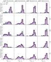 |
Fig. A.1. Application of our method to the sample of galaxies in and around X-ray clusters used by Martínez et al. (2023). As in Fig. 2, rows show different classes, and columns different stellar mass ranges. Green shaded histograms are predicted colour distributions and violet shaded histograms recovered colour distributions. |
All Figures
|
Fig. 1. Confusion matrix for our adopted classification scheme (Coenda et al. 2022). Columns correspond to intrinsic classes, rows to predicted classes. |
| In the text | |
|
Fig. 2. Colour distributions of galaxies. Each class is shown in a different row, as noted to the right of the panels. Each column considers a particular range of galaxy stellar mass, as noted at the top. Grey shaded histograms are the real colour distributions, i.e. they correspond to the intrinsic classes. Green lines are the colour distributions of the predicted classes. Violet lines are the colour distributions recovered by our method. We quote within each panel the values of the corresponding square residuals, Spred and Srec, given by Eqs. (6) and (7), respectively. |
| In the text | |
|
Fig. 3. Sum of square residuals as a function of galaxy stellar mass. Each panel considers a different galaxy class. Residuals between the real and the predicted distributions are shown with green lines, i.e. Spred in Eq. (6). Residuals between the real and the recovered distributions are shown with violet lines, i.e. Srec in Eq. (7). The residuals between the real and the recovered distributions when we use a stellar mass-dependent confusion matrix are shown in orange. Note that the y-axis scale varies from panel to panel. |
| In the text | |
|
Fig. A.1. Application of our method to the sample of galaxies in and around X-ray clusters used by Martínez et al. (2023). As in Fig. 2, rows show different classes, and columns different stellar mass ranges. Green shaded histograms are predicted colour distributions and violet shaded histograms recovered colour distributions. |
| In the text | |
Current usage metrics show cumulative count of Article Views (full-text article views including HTML views, PDF and ePub downloads, according to the available data) and Abstracts Views on Vision4Press platform.
Data correspond to usage on the plateform after 2015. The current usage metrics is available 48-96 hours after online publication and is updated daily on week days.
Initial download of the metrics may take a while.