| Issue |
A&A
Volume 691, November 2024
|
|
|---|---|---|
| Article Number | A79 | |
| Number of page(s) | 10 | |
| Section | Numerical methods and codes | |
| DOI | https://doi.org/10.1051/0004-6361/202451707 | |
| Published online | 31 October 2024 | |
On thermal conduction in the solar atmosphere: An analytical solution for nonlinear diffusivity without compact support
1
Rosseland Centre for Solar Physics, University of Oslo,
PO Box 1029
Blindern,
0315
Oslo,
Norway
2
Institute of Theoretical Astrophysics, University of Oslo,
PO Box 1029
Blindern,
0315
Oslo,
Norway
3
Lockheed Martin Solar and Astrophysics Laboratory,
3251 Hanover Street,
Palo Alto,
CA
94304,
USA
4
Bay Area Environmental Research Institute,
NASA Research Park,
Moffett Field,
CA
94035,
USA
★ Corresponding author; sondrevf@uio.com
Received:
29
July
2024
Accepted:
17
September
2024
Context. The scientific community employs complicated multiphysics simulations to understand the physics in solar, stellar, and interstellar media. These must be tested against known solutions to ensure their validity. Several well-known tests exist, such as the Sod shock tube test. However, a test for nonlinear diffusivity is missing. This problem is highly relevant in the solar atmosphere, where various events release energy that subsequently diffuses by Spitzer thermal conductivity.
Aims. The aim is to derive an analytical solution for nonlinear diffusivity in 1D, 2D, and 3D, which allows for a nonzero background value. The solution is used to design a test for numerical solvers and study Spitzer conductivity in the solar atmosphere.
Methods. There exists an ideal solution assuming zero background value. We performed an analytical first-order perturbation of this solution. The first-order solution was first tested against a dedicated nonlinear diffusion solver, whereupon it was used to benchmark the single- and multifluid radiative magnetohydrodynamics code Ebysus, used to study the Sun. The theory and numerical modeling were used to investigate the role of Spitzer conductivity in the transport of energy released in a nanoflare.
Results. The derived analytical solution models nonlinear diffusivity accurately within its region of validity and approximately beyond. Various numerical schemes implemented in the Ebysus code is found to model Spitzer conductivity correctly. The energy from a representative nanoflare is found to diffuse 9 Mm within the first second of its lifetime due to Spitzer conductivity alone, strongly dependent on the electron density.
Conclusions. The analytical first-order solution is a step forward in ensuring the physical validity of intricate simulations of the Sun. Additionally, since the derivation and argumentation are general, they can easily be followed to treat other nonlinear diffusion problems.
Key words: conduction / diffusion / magnetohydrodynamics (MHD) / methods: analytical / methods: numerical / Sun: flares
© The Authors 2024
 Open Access article, published by EDP Sciences, under the terms of the Creative Commons Attribution License (https://creativecommons.org/licenses/by/4.0), which permits unrestricted use, distribution, and reproduction in any medium, provided the original work is properly cited.
This article is published in open access under the Subscribe to Open model. Subscribe to A&A to support open access publication.
1 Introduction
The scientific community of today relies heavily on complicated multiphysics simulations. To increase the trustworthiness of such simulations, every single physics module should be benchmarked against analytical solutions. Several such benchmarks exist and are often used, such as the Sod shock tube test for hydrodynamics codes (Sod 1978).
In this paper, we are interested in partial differential equations of parabolic terms (nonlinear diffusion) in Cauchy problems. Assuming radial symmetry, that is given by
 (1)
(1)
where K is a constant, n > 0 is the (positive) nonlinearity exponent, and s ∈ (1,2,3) is the number of dimensions. T is chosen because it later in this paper represents temperature, but it can represent any value. A diverse set of problems can be modeled by such nonlinear diffusion with different exponents n, an inexhaustive list is given by Diez et al. (1992).
It is computationally demanding to solve such problems numerically. That is because the stability condition of an explicit diffusion solver requires the time step to scale like the spatial resolution squared, ∆t ∝ ∆r2 (see Press et al. 2007, p. 1044).
Therefore, different algorithms have been developed over the years to solve such problems and bypass this time-step constraint. These algorithms need to be tested, preferably against an analytical solution.
An analytical solution exists for nonlinear diffusion of an instantaneous point source with zero background T, making the diffusion coefficient in Eq. (1) equal to zero beyond the extent of the point source (Pattle 1959). That derivation finds self-similar solutions that keep their shape with a gradually lower peak value and broader spatial extent with time. In some problems, however, it is not realistic to have zero background value. In this paper, we extend this theory by a perturbation to include a nonzero background value. The theory is used to analyze the efficacy of different numerical schemes.
We apply the derivation to the modeling of thermal conductivity by electrons in a plasma, as in the solar atmosphere (Spitzer 1962). If we assume a negligible heat conduction perpendicular to the magnetic field in the plasma and a constant mass density ρ, the conductive term can be written on the form (see App. A for details)
 (2)
(2)
where cv is the specific heat capacity per mass, ρ is the mass density, and  is the parallel thermal conductivity with exponent
  . Since the conduction is along the field lines, this is modeled as diffusion in s = 1 dimensions. The coefficient in the thermal conductivity is
  for a fully ionized hydrogen gas in the solar atmosphere (Spitzer 1962; Priest 1984). To bypass the time step constraint of typical explicit methods, this term can be solved implicitly as in Bifrost (Gudiksen et al. 2011), with the wave method first implemented in MURaM (Rempel 2016), or the explicit orthogonal Chebyshev method known as ROCK2 (Abdulle & Medovikov 2001; Abdulle 2002; Abdulle & Li 2008; Zbinden 2011) and implemented in Ebysus (Martínez-Sykora et al. 2020).
One cannot reasonably assume a zero background temperature when modeling the nonlinear thermal conductivity in the solar atmosphere. However, the background temperature can be much smaller than the source temperature, for example when modeling thermal conduction from the O(MK) corona to the O(kK) photosphere or when modeling the localized release of energy from a nanoflare, as described and studied numerically by Testa et al. (2014); Polito et al. (2018); Bakke et al. (2022). Polito et al. (2018) found that lower-energy electrons tend to release more energy in the corona than higher-energy electrons, as previously found in Reep et al. (2015), but that thermal conduction is more effective at heating the magnetic loop. Further, they found that the initial conditions (IC) of the loops prior to a nanoflare, in particular temperature and density, significantly impact the atmosphere’s response. This work was extended into stellar flare events, where thermal conduction is more important than radiation and a key process in the energy flux (Kowalski et al. 2024). These studies model several physical processes that play a role in the energy flux in flares to get a realistic description, including electron beams, thermal conductivity, nonlocal thermal equilibrium, and radiation. Each of these processes competes and it is crucial to understand their independent solutions to understand and separate their contributions. We focus on the role of thermal conductivity.
In this paper, we first make an analytical solution of the nonlinear diffusivity in Sect. 2, which we verify numerically in Sect. 3. Based on this, we explain and show how to use this derivation to benchmark a code in Sect. 4. Then, we make a numerical experiment of how fast energy diffuses from a nanoflare in Sect. 5 before we conclude.
2 Analytical derivation
2.1 Solution with zero background, T∞=0
An initial instantaneous point source quantity ϕ0 released at t = 0 and centered at r0 = 0 diffuses as the self-similar solutions first described by Pattle (1959) and comprehensively derived in App. B. If we allow for a finite initial extent, they can be written as
 (3)
(3)
 (4)
(4)
 (5)
(5)
where T0 = max[T(t = 0)] is the initial representative peak value and R0 is the initial representative width beyond which T = 0.
Self-similar shapes for various n in s = 1 dimensions are displayed in Fig. 1. The initial peak and width are related to the total quantity (area under the graph) by
 (6)
(6)
where Ωs = {2,2π, 4π} is the solid angle for s = {1,2,3} dimensions,  is Euler’s Beta integral (see Abramowitz & Stegun 1965, ch. 6), and Gs,n ≲ 1 (for n ≥ 1) is a time-independent geometrical factor depending on n and s.
The representative peak T0 and width R0 are not clearly defined for an instantaneous point source. However, that is not a severe problem as any distribution that is 0 beyond a finite radius eventually approaches the shape in Eq. (3). This can be understood by taking the limit χt >> 1, corresponding to R0 → 0, and using Eq. (6), to get
 (7)
(7)
 (8)
(8)
The distribution depends only on the initial total quantity ϕ0, not T0 and R0. The peak and width have simple dependencies on time, ![$\max [T] \propto {t^{ - {s \over {sn + 2}}}}{\rm{ and }}R \propto {t^{{1 \over {sn + 2}}}}$](/articles/aa/full_html/2024/11/aa51707-24/aa51707-24-eq13.png) , making ϕ(t) = max[T(t)]R(t)s/Gs,n a constant.
, making ϕ(t) = max[T(t)]R(t)s/Gs,n a constant.
For comparison, in the limiting case n = 0, corresponding to isotropic diffusion (D = K), an initial instantaneous point source at r0 = 0 is known to diffuse as a Gaussian that can be written as
 (9)
(9)
 (10)
(10)
 (11)
(11)
Here, Rσ(t) is the standard deviation of the Gaussian distribution, not the boundary beyond which T = 0, since the Gaussian extends to infinity. The total quantity is
 (12)
(12)
We can see by the self-similar shapes in Fig. 1 that the Gaussian distribution is the limiting case for n → 0+. As n → ∞, the edges become sharper as the diffusion coefficient in Eq. (1) is relatively stronger at larger values, making the geometrical factor G1,n → 1/Ω1 = 0.5 in s = 1 dimensions.
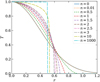 |
Fig. 1 Illustration of self-similar solutions in s = 1 dimensions for different n given by the legend. All solutions have peak value T0 = 1 and total quantity ϕ0 = 1, being symmetric around r = 0. |
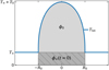 |
Fig. 2 Illustration of ICs with a background value T∞ ≥ 0 for s = 1 dimensions and n = 5/2. |
2.2 Including a nonzero background, T∞ > 0
The aim of this paper is to include a background value T∞ and then predict how it evolves. By assuming that the background has had time to reach equilibrium, we set T∞ to a constant. That is, however, not essential for the following arguments. The total initial distribution is given by
 (13)
(13)
as illustrated in Fig. 2. If one completely neglects the impact of the background value and assumes that the source evolves as before, one gets the ideal zeroth-order solution
 (14)
(14)
where the superscript (0) marks the zeroth order. This is a too naïve approach. An important assumption in the ideal derivation in App. B (based on Pattle 1959) was that T eventually would go to zero beyond a finite radius, given by Eq. (B.3). That assumption is broken by including a background value T∞ > 0. By understanding the derivation in App. B, we realize in the following the importance of this constraint and the consequences of breaking it.
The shape of T(r, t) for r < R(t), given by Eq. (3), solves the nonlinear diffusion equation in Eq. (1). Alternative solutions include the trivial solution T = 0 and constant solution T = const > 0. The trivial solution has the important added benefit that it makes the diffusion coefficient in Eq. (1) zero, perfectly separating the two regions at the boundary r = R(t). A nonzero background distribution T∞ > 0 causes diffusion out beyond R(t), preventing the perfect separation of the two regions.
We considered first the case T∞ >> T0. This allowed a Taylor expansion of the diffusion coefficient around the background as
![$\matrix{ {D\left( {{T_{{\rm{Tot}}}}} \right) = K{{\left( {{T_\infty } + T} \right)}^n}} \hfill \cr { & = KT_\infty ^n\left[ {1 + n{T \over {{T_\infty }}} + {{n(n - 1)} \over 2}{{{T^2}} \over {T_\infty ^2}} + O\left( {{{{T^3}} \over {T_\infty ^3}}} \right)} \right].} \hfill \cr } $](/articles/aa/full_html/2024/11/aa51707-24/aa51707-24-eq20.png) (15)
(15)
This diffusion is dominated by the first term, which is constant. The second term gradually becomes less important as max[TTot(t)] decreases toward T∞. Hence, the source immediately diffuses into the Gaussian shape in Eq. (9).
We considered next the case T∞ << T0, which was less trivial and more interesting for our use case. It was tempting to make a similar expansion as in Eq. (15), with T and T∞ exchanged, giving terms of Tn, Tn−1, etc. That expansion is valid at r << R, where T >> T∞. The nonzero background value causes a slightly larger diffusion coefficient, making the peak value max[TTot] drop slightly faster. However, at r → ∞, the instantaneous point source has not yet diffused, making T = 0 << T∞ and the expansion singular. In the intermediate region, at r ~ R, the background and source become comparable, T ~ T∞, making the terms of different order in T comparable as well. Thus, the distribution does not have as sharp edges as for n > 1 in Fig. 1, it has wider tails as for smaller values of n → 0. Nevertheless, by considering the inverse time scales χ in Eq. (5), which is proportional to the peak diffusion coefficient, we found that the global widening was still dominated by the Tn term. Hence, the overall widening follows the n-solution, but it is reshaped to have wider tails. Nevertheless, as χt → ∞, the peak value eventually drops to max[T(t)] << T∞, and it diffuses into a Gaussian, as for the previous case, T∞ >> T0.
2.3 First-order solution for T∞ ≪ T0
In the previous section, we discussed qualitatively how the solution changes when adding a nonzero background value T∞ > 0. In this section, we derive a first-order perturbation solution that quantitatively estimates it. This is done assuming an identical shape to the ideal solution but with a modified peak and width. We consider separately the two time regimes, χt << 1 and xt >> 1. In the former, the zeroth-order solution depends on the shape of the IC, while in the latter, only on the source quantity ϕ0.
We considered first xt << 1, the beginning of the diffusion. In this regime, we focused on how the peak value max[TTot] evolved. The peak of the zeroth-order solution in Eq. (14) is given by
![$\max \left[ {T_{{\rm{Tot}}}^{(0)}(t)} \right] = {T_\infty } + T(0,t) = {T_\infty } + {T_0}{\left[ {1 + \chi \left( {{T_0}} \right)t} \right]^{ - {s \over {sn + 2}}}},$](/articles/aa/full_html/2024/11/aa51707-24/aa51707-24-eq21.png) (16)
(16)
where the dependence on T0 in χ from Eq. (5) was made explicit. The first-order perturbation is to include the background value in χ as
![$\matrix{ {\max \left[ {T_{{\rm{Tot}}}^{(1)}(t)} \right] = {T_\infty } + {T_0}{{\left[ {1 + \chi \left( {{T_0} + {T_\infty }} \right)t} \right]}^{ - {s \over {sn + 2}}}}} \hfill \cr {\,\,\,\,\,\,\,\,\,\,\,\,\, = {T_\infty } + {T_0}{{\left[ {1 + {{\left( {1 + {{{T_\infty }} \over {{T_0}}}} \right)}^n}\chi \left( {{T_0}} \right)t} \right]}^{ - {s \over {sn + 2}}}}.} \hfill \cr } $](/articles/aa/full_html/2024/11/aa51707-24/aa51707-24-eq22.png) (17)
(17)
We expanded the parentheses by taking the limits χt << 1 and T∞ << T0 to get a simple algebraic expression for the correction done by the first perturbation
![$\max \left[ {T_{{\rm{Tot}}}^{(1)}(t)} \right] - \max \left[ {T_{{\rm{Tot}}}^{(0)}(t)} \right] \approx - {{sn} \over {sn + 2}}{{{T_\infty }} \over {{T_0}}}\chi \left( {{T_0}} \right)t.$](/articles/aa/full_html/2024/11/aa51707-24/aa51707-24-eq23.png) (18)
(18)
The correction is negative, meaning that the extra diffusion due to the background makes the peak decrease faster, as expected. Furthermore, it is also proportional to χ(T0)t and T∞/T0, which are assumed to be small in this regime. In the following, χ always means χ(T0), as in Eq. (5).
We considered next χt >> 1. In this regime, we focus first on the solution’s width. As seen from Eq. (8), the widening to zeroth order depends on ϕ0. However, this expression neglects ϕ∞ that is illustrated in Fig. 2, which corresponds to the background and increases with time as
 (19)
(19)
To first order, we used the unperturbed radius R(0) to approximate the extra quantity ϕ∞, which gave
 (20)
(20)
The correction is positive, meaning that the background causes the distribution to widen faster. The relative correction is proportional to T∞/T0, which is small, and to (R(0)(t)/R0)s, which gradually increases. Even though the limit ϕ∞ << ϕ0 is only taken for the final right-hand side (RHS) of Eq. (20), this first-order correction is erroneous when ϕ∞ ≳ ϕ0.
To make the expression in Eq. (20) approximately valid for χt ≲ 1, we did an approximate asymptotic matching by reintroducing the 1 in the parenthesis of Eq. (4)
![${R^{(1)}}(t) = {R_0}{\left[ {1 + {{\left( {{{{\phi _{{\rm{Tot}}}}} \over {{\phi _0}}}} \right)}^n}\chi t} \right]^{{1 \over {s\,n + 2}}}}$](/articles/aa/full_html/2024/11/aa51707-24/aa51707-24-eq26.png) (21)
(21)
We now have the expression ![$\max \left[ {T_{{\rm{Tot}}}^{(1)}(t)} \right]$](/articles/aa/full_html/2024/11/aa51707-24/aa51707-24-eq27.png) for χt << 1 and R(1)(t) for χt >> 1. To complete the pairs, we used that the total quantity above T∞ was still equal to ϕ0 as in Eq. (6), enforced by setting
for χt << 1 and R(1)(t) for χt >> 1. To complete the pairs, we used that the total quantity above T∞ was still equal to ϕ0 as in Eq. (6), enforced by setting ![$\left( {\max \left[ {T_{{\rm{Tot}}}^{(1)}(t)} \right] - {T_\infty }} \right){\left( {{R^{(1)}}(t)} \right)^s} = {T_0}R_0^s$](/articles/aa/full_html/2024/11/aa51707-24/aa51707-24-eq28.png) . That gave
. That gave
![$\max \left[ {T_{{\rm{Tot}}}^{(1)}(t)} \right] = \left\{ {\matrix{ {{T_\infty } + {T_0}{{\left[ {1 + {{\left( {1 + {{{T_\infty }} \over {{T_0}}}} \right)}^n}\chi t} \right]}^{ - {s \over {s\,n + 2}}}}} \hfill & {{\rm{, if }}\chi t \ll 1} \hfill \cr {{T_\infty } + {T_0}{{\left[ {1 + {{\left( {{{{\phi _{{\rm{Tot}}}}} \over {{\phi _0}}}} \right)}^n}\chi t} \right]}^{ - {s \over {s\,n + 2}}}}} \hfill & {,{\rm{ if }}\chi t \mathbin{\lower.3ex\hbox{\buildrel>\over {\smash{\scriptstyle\sim}\vphantom{_x}}}} 1} \hfill \cr { \to {T_\infty } + {{\left( {{n \over {sn + 2}}{{{{\left( {{G_{s,n}}{\phi _{{\rm{Tot}}}}} \right)}^{{2 \over s}}}} \over {2Kt}}} \right)}^{{s \over {s\,n + 2}}}}} \hfill & {{\rm{, if }}\chi t \gg 1} \hfill \cr } } \right.$](/articles/aa/full_html/2024/11/aa51707-24/aa51707-24-eq29.png) (22)
(22)
![${R^{(1)}}(t) = \{ \matrix{ {{R_0}{{\left[ {1 + {{\left( {1 + {{{T_\infty }} \over {{T_0}}}} \right)}^n}\chi t} \right]}^{{1 \over {sn + 2}}}}} \hfill & {,{\rm{if}}\chi t \ll 1} \hfill \cr {{R_0}{{\left[ {1 + {{\left( {{{{\phi _{{\rm{Tot}}}}} \over {{\phi _0}}}} \right)}^n}\chi t} \right]}^{{1 \over {sn + 2}}}}} \hfill & {,{\rm{if}}\chi t \mathbin{\lower.3ex\hbox{\buildrel>\over {\smash{\scriptstyle\sim}\vphantom{_x}}}} 1} \hfill \cr { \to {{\left( {{{sn + 2} \over n}2K{{\left( {{G_{s,n}}{\phi _{{\rm{Tot}}}}} \right)}^n}t} \right)}^{{1 \over {sn + 2}}}}} \hfill & {,{\rm{if}}\chi t \gg 1.} \hfill \cr } $](/articles/aa/full_html/2024/11/aa51707-24/aa51707-24-eq30.png) (23)
(23)
Only the second term of ![$\max \left[ {T_{{\rm{Tot}}}^{(1)}(t)} \right]$](/articles/aa/full_html/2024/11/aa51707-24/aa51707-24-eq31.png) , not T∞, should be multiplied by [1 − (r/R(1))2]1/n as in Eq. (3).
, not T∞, should be multiplied by [1 − (r/R(1))2]1/n as in Eq. (3).
Parameters for numerical verification of theory.
2.4 Validity and limitations of the first-order solution
The first-order solutions in Eqs. (22)–(23) are adjustments of the zeroth-order solutions in Eqs. (4) and (14). At large times χt >> 1, the adjustments stem from expanding the quantity ϕ0 by ϕ∞, equivalent to a factor (1 + ϕ∞/ϕ0). One can imagine that a second-order solution would include an additional term of order (ϕ∞/ϕ0)2. For an exponent α ≲ 1, being  for the width and peak, respectively, the adjustment becomes
 (24)
(24)
The 2nd and 3rd terms on the RHS stem from the first-order perturbation, estimating the modification by the first-order perturbation. The 4th term estimates the modification by the second-order perturbation. It is this term that must be small for the first-order perturbation to be a good approximation. The 5th term of higher order reminds us that these perturbation expressions are not valid estimates when ϕ∞ ~ ϕ0 in general.
This first-order solution also has a significant limitation. It modifies the peak and width but assumes the zeroth-order shape. In Section 2.2, we argued that the background modifies the shape to have wider tails. Therefore, we expect an unrepresentative larger error for the boundary R beyond which TTot = T∞. Instead, we study the evolution of Rp, defined as the radius where the source has height equal to p times the peak value above the background
![${T_{{\rm{Tot}}}}\left( {{R_p},t} \right) = {T_\infty } + p\left( {\max \left[ {{T_{{\rm{Tot}}}}(t)} \right] - {T_\infty }} \right).$](/articles/aa/full_html/2024/11/aa51707-24/aa51707-24-eq34.png) (25)
(25)
A common example of this is the half-width-half-maximum (HWHM), given by p = 0.5. Since these are self-similar shapes, both R(t)/R(0) and Rp(t)/Rp(0) have the same time dependence, given by Eq. (4) in the limit T∞ → 0+.
3 Numerical validation of perturbation theory
We ran a controlled numerical experiment to test the analytical expressions for the ideal solution T(0) and first-order solution T(1). This was done for the normalized parameters presented in Table 1, including three different values for T∞, all smaller than T0. The exponent n = 5/2 and dimensionality s = 1 correspond to thermal conductivity in the solar corona, as described in Section 1. The initial quantity was calculated from Eq. (6) to be ϕ0 ≈ 1.64. The exponent α in Eq. (24) takes the values  and
and  for the width and peak, respectively.
The numerical results were calculated with an implicit scheme (BDF), using scipy.solve_ivp in Python with the second-order stencil
![${{\partial {T_i}} \over {\partial t}} = {K \over {\Delta r}}\left[ {{{T_{\,i + 1}^n + T_i^n} \over 2}{{{T_{i + 1}} - {T_i}} \over {\Delta r}} - {{T_i^n + T_{i - 1}^n} \over 2}{{{T_i} - {T_{i - 1}}} \over {\Delta r}}} \right],$](/articles/aa/full_html/2024/11/aa51707-24/aa51707-24-eq37.png) (26)
(26)
using ∆r = R0/250 = 4 × 10⁻³. Hence, the initial peak was sufficiently well resolved to make numerical artifacts negligible.
The results of the scan are presented in Fig. 3. The calculations were run equally long, until a time t′ such that ϕ∞(t′) = ϕ0 in Fig. 3c. This occurs when the zeroth-order radius is R(0)(t′) = 16.35 R0, which is in the regime χt >> 1. Hence, it is the perturbation in the second line of Eq. (23) that was compared to the simulation. For the first case, T∞/T0 = 0.001, the final background quantity is negligible compared to the source quantity, ϕ∞(t′)/ϕ0 = 0.02. Hence, the zeroth- and first-order solutions are visually almost indistinguishable as the peak and width are adjusted by approximately 1%. Compared to the simulation, the relative error of the peak decreases significantly from 1% to 0.1%. For the second case, T∞/T0 = 0.01, the ideal and first-order solutions have visually diverged. It is the latter that best approximates the simulation. The extra quantity is still small but nonnegligible, ϕ∞(t′)/ϕ0 = 0.20. In this case, the width has increased by 11% due to the first-order perturbation, while the estimated second-order correction in Eq. (24) is only 2.2%. The peak value ![$\max \left[ {T_{{\rm{Tot}}}^{(1)}(t)} \right]$](/articles/aa/full_html/2024/11/aa51707-24/aa51707-24-eq38.png) and HWHM are almost identical to the simulation. However, the expected slightly heavier tail in the simulation is visible. For the third case, T∞/T0 = 0.05, the extra quantity has reached equality to the source quantity, ϕ∞(t’) = ϕ0. Even though the first-order solution is better than the ideal case, it is no longer a good approximation of the simulation. Both the peak and HWHM are visually different, and the shape is even more different. This was expected, as second- and higher-order terms of (ϕ∞(t’)/ϕ0) = 1, is no longer negligible.
and HWHM are almost identical to the simulation. However, the expected slightly heavier tail in the simulation is visible. For the third case, T∞/T0 = 0.05, the extra quantity has reached equality to the source quantity, ϕ∞(t’) = ϕ0. Even though the first-order solution is better than the ideal case, it is no longer a good approximation of the simulation. Both the peak and HWHM are visually different, and the shape is even more different. This was expected, as second- and higher-order terms of (ϕ∞(t’)/ϕ0) = 1, is no longer negligible.
We studied the time evolution in greater detail for the intermediate background value, T∞/T0 = 0.01. The evolution of max[T] and the HWHM (R0.5) are presented in Fig. 4. The absolute value curves in the first panel are visually indistinguishable, except the ideal zeroth-order solution that deviates toward the end with a too narrow and peaked distribution, as expected. After χt = 10, the peak error levels out at almost 6 × 10⁻³ T0. It does not grow more for these parameters because the simulation is slower for a smaller peak and both peaks decrease toward max[TTot] → T∞ = 10−2 T0. However, the relative error in width ends at −16%.
The first-order perturbation has three different curves, depending on the value of χt. They are given in the same order by the legend as by the three lines in Eqs. (22)–(23). The third line only coincides with the second for χt > 103. This delayed convergence supports the need for the approximate matching introduced in Eq. (21). The second line also coincides rather well with the first line for χt < 0.1, and thereby connecting the two regimes. Therefore, only the second expression is used in the following sections.
The first-order perturbation reduces the differences between the simulation and the ideal zeroth-order solution up to the end of the simulation when ϕ∞/ϕ0 = 0.4. The absolute relative peak error maxes at 5 × 10⁻⁴ T0, an order of magnitude smaller than before. The relative width error has also dropped by an order of magnitude, to 1.6% at the end of the simulation, notably now with the opposite sign.
Counterintuitively, the ideal zeroth-order solution appears to better estimate the width at small times χt < 0.3, as seen in the bottom panel of Fig. 4. However, these small errors are, first of all, relative to the ideal HWHM, which is initially small as well. The relative mismatch decreased by reducing the grid spacing ∆r to the current choice, as the singular point at r = R is difficult to resolve with a uniform grid. Here, the absolute difference to the first-order perturbation is approximately ∆r/4. Secondly, the distribution shape is expected to adjust during this time regime, χt ≪ 1. By close inspection, the discrepancy to the first-order perturbation is caused by the marginally heavier tails in the simulation, making the width at half maximum marginally narrower. This effect is illustrated by comparing the curves for  and, for example, n = 0 in Fig. 1.
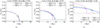 |
Fig. 3 Verification of analytical derivation. Each plot shows the IC, as well as the simulation run using solve_ivp in Python, zeroth-order solution T(0), and first-order solution T(1), all at a later time such that χt >> 1. The colored ‘+’ corresponds to the HWHM point of each calculation. This is done for increasing background values T∞/T0 given by the plot titles. The simulation box extends to r = 100 R0 in (c), preventing any impacts caused by the boundary condition. |
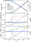 |
Fig. 4 Verification of analytical derivation for T∞/T0 = 0.01. Comparison as a function of χt for a simulation in Python (blue markers), as well as the zeroth-order (magenta curve) and first-order solutions (three green curves). In the top panel, the absolute reduction of max[TTot] and widening of HWHM (R0.5) is shown. In the following two panels, the difference to the simulation is shown for the peak temperature and width, respectively. These panels also include the evolution of ϕ∞/ϕ0 in black. The dashed vertical line marks t = 1/χ and the dotted vertical line marks t = t’ >> 1/χ, the time of the snapshot in Fig. 3b. |
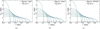 |
Fig. 5 Comparison between Ebysus and the first-order expression in Eqs. (22)–(23). The narrowest curve is the IC, and the following curves are given after exponentially longer time as [3 s, 6 s, 12 s, … ]. Ebysus was run with different Spitzer methods in the different panels: (a) is explicit, (b) is the wave method from Rempel (2016), and (c) is the ROCK2 method (Abdulle & Medovikov 2001). |
4 Benchmarking a numerical code
4.1 Designing a numerical test
The previous sections illustrate several requirements to remember when designing a test for a nonlinear diffusion solver for any exponent n.
-
α(ϕ∞/ϕ0)1 ≪ 1, if zeroth-order solution
α(ϕ∞/ϕ0)2 ≪ 1, if first-order solution
where

χt ≫ 1

R0 ≫ ∆r
Point 1 states that one must use the zeroth and first-order solutions only in their regions of validity. This sets an upper limit for the time. Point 2 incorporates that one additionally must wait until the initial distribution has adjusted to the approximately self-similar solution, setting as well a lower limit for time. Obviously, the lower limit for time must be lower than the upper limit. When it comes to spatial discretization, the lower limit on time from point 2 also sets a lower limit for how much the distribution has to widen, given by point 3. Point 4 includes additionally that the initial distribution must be sufficiently resolved numerically. The latter two points combined make a lower requirement for how many grid points one needs. A functioning set of parameters for this is given by the parameters in Table 1, with T∞/T0 ≤ 0.01 and R0/∆r ≥ 10, run until a time t′ such that R(0)(t′)/R0 ≥ 2, but also ϕ∞(t′)/ϕ0 ≤ 0.10. This can be both a one-off test, as exemplified below, or continuous integration in the form of a test to be automatically run at each new commit to a version control software such as git.
4.2 Test of Spitzer conductivity in Ebysus
The theory described in this paper was used to benchmark various solvers for Spitzer conductivity implemented in Ebysus. The benchmark was done for a one-off case with parameters comparable to those in the solar atmosphere. The electron density was N = 1 × 1012 cm−3 and the conductivity coefficient was set to  erg s−1 cm−1 K−35, which is realistic for the solar atmosphere (Braginskii 1965; Spitzer 1962). The background temperature combined with the released energy gave an initial temperature profile as in Eq. (14) with T∞ = 5 × 10⁴ K, T0 = 5 × 10⁶ K, and R0 = 225 km.
The comparison to the first-order solution is given as a function of the radius in Fig. 5. The agreement is clear. Toward the end, the tails are slightly wider in the simulations compared to the theory, as expected from theoretical considerations in Sect. 2.2 and also seen in Fig. 3.
The corresponding errors of the peak and HWHM are given in Fig. 6. All three methods agree reasonably well, the wave method being slightly off compared to the other two. The error seems to grow with time, especially for the HWHM. Since the first-order solution shows a lower peak value and larger HWHM than the trusted simulation in Fig. 4, one can argue that the explicit and ROCK2 methods are more accurate than the wave method. This is understandable since the wave method approximates the problem by solving a hyperbolic diffusion equation (Rempel 2016).
To advance the simulations 3 s from the IC to the second curve in Fig. 5 or first point in Fig. 6, the standard explicit method used 28656 time steps, the wave method used 7111 time steps, while the ROCK2 method used 2699 time steps. The length of the time steps was calculated dynamically to ensure numerical stability, depending on the diffusivity D(T) and the spatial resolution. These numbers exemplify that many time steps are required to solve nonlinear diffusion and that great speedup can be achieved by seeking alternatives to the standard explicit method, such as the competitive wave and ROCK2 methods. Wargnier et al. (2024) will describe further details on the Ebysus benchmark using both ROCK2 and a partitioned implicit-explicit orthogonal Runge-Kutta method called PIROCK (Abdulle & Vilmart 2013). Furthermore, Cherry et al. (2024) will use the theory derived here to study the Spitzer conductivity modeling in the Bifrost code, aiming to analyze the efficacy of the different numerical methods.
It is important to verify that these tests followed the benchmark requirements given in Sect. 4.1. The final distribution is well within the first requirement, with ϕ∞/ϕ0 = 0.05 ≪ 1 and α ∊ {5/9, 4/9}. The curves shown, except for the IC, are for t ≥ 3.0 s ≫ 1/χ = 0.47 s. As a consequence, their widths R(t > 0) are significantly larger than R0. Even larger widths could have been necessary if not for the choice of setting the IC equal to the relevant self-similar solution. There is no concrete estimate for when a general source distribution reaches the self-similar solutions, even in the ideal case. Lastly, the IC is well resolved, with resolution such that R0/∆r = 100 ≫ 1.
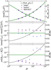 |
Fig. 6 Error plot for the test of Ebysus presented in Fig. 5. See the description in the similar Fig. 4. Here, several y axes are linear and the error is shown relative to the first-order perturbation theory. The symmetric logarithmic error scales in the two bottom panels go from −4 × 10⁻² to 4 × 10⁻². |
5 Nanoflare experiment
Finally, we analyzed the thermal Spitzer conductivity during nanoflares in the solar atmosphere in isolation from other physical processes. We were inspired by the studies of Polito et al. (2018) and Testa et al. (2014). Here, we focus on the impact of only conductivity without radiation, nonequilibrium ionization effects, advection, or electron beams. A total of 10 configurations were analyzed, consisting of 1 reference model and 9 variations where we studied the impact of changing different key parameters focusing solely on thermal conduction.
5.1 Model setup
A reference experiment was constructed similar to the thermal conduction experiment in Polito et al. (2018) with an initial peak temperature of 1 MK and coronal electron density of N ≲ 1 × 109 cm−3. They increased the energy by  erg s−1 for 10 s over an area of A = 5 × 1014 cm2 (corresponding to a diameter of 0.25 Mm) transverse to the magnetic field and over a length of 9 Mm along a magnetic loop. This is appropriate for a nanoflare according to the work of Testa et al. (2014) and the description of nanoflares by Parker (1988). The released energy increases the coronal temperature to 20 MK in a few seconds. The energy is conducted down to the transition region, which causes the denser plasma to move quickly up into the corona.
Our study focuses on the importance of thermal conduction at the beginning of a nanoflare, and how it depends on the key parameters. Spitzer’s conductivity coefficient was again set to  erg s−1 cm−1 K−3.5 (Braginskii 1965; Spitzer 1962). The IC of the reference experiment was consistent with an immediate energy increase equivalent to a typical nanoflare energy release over 1 s,
  erg. All the energy was unrealistically assumed to increase the temperature of the plasma, no energy went into macroscopic kinetic energy or ionization. The energy was released over an area A = 5 × 1014 cm2 transverse to the magnetic field and over a self-similar shape with radius
  Mm parallel to the magnetic field, corresponding to an effective diameter of 0.25 Mm. The reference electron density was set to Nref = 1 × 109cm−3. Assuming an ideal gas, that gives an initial peak temperature of
  MK that quickly diffuses over the background temperature of
  MK. Even though this peak temperature is unrealistic, we chose such a large
  and correspondingly small
  to illustrate the impact of different key parameters better.
In addition to the reference experiment, several small parameter scans were performed around the reference parameters 
Change T0 and R0 ∝ 1/T0 with E unchanged.
Change T0 and E ∝ T0 with R0 unchanged.
Change only T∞.
Change N with E unchanged, which in turn changes both T0 ∝ 1/N and the
 in Eq. (2).
5.2 Results
The numerical experiments were simulated with the code described in Sect. 3 with R0/∆r ≥ 25 and evaluated with the first-order theory described in Eqs. (22–23). The evolution of the HWHM R0.5 (radius at 50% of maximum) and maximum temperature max[TTot] are presented in Fig. 7. The theoretical curves agree well with the simulations in most cases. For the encircled points, marking when ϕ∞ ≥ ϕ0, the agreement becomes worse, as expected. This is due to the heavier tails illustrated in Fig. 3c that are not properly represented outside the region of validity of the first-order solution. The general behavior is, nevertheless, well described by the analytical first-order solutions.
The reference simulation shows the behavior due to the conduction of energy released in the first second of a nanoflare in the corona. Within 1 s, the energy is spread out over an area with HWHM of approximately 9 Mm, or full width of 18 Mm, and the maximum temperature has dropped to 2MK = 2 T∞. Hence, the extent of the coronal heating used in Polito et al. (2018) can be achieved by the conduction alone within a second.
When varying the parameters from those of the reference configuration, several important results are prominent, many of which can be understood from the analytical solution. Changing only T0 and R0 affects only the early phase of the evolution. At χt ≫ 1, these curves converge to the reference configuration. Hence, the spatial extent of the IC parallel to the magnetic field is of little physical importance for long-term conductivity.
Increasing T0 and E, while keeping R0 fixed, causes a larger χ in Eq. (5) and thereby an earlier evolution since χt = 1 occurs for a correspondingly earlier t. Hence, the energy of a more energetic event is conducted faster. Changing the released energy by an order of magnitude up (down), as in the scan, changes both the radius and the temperature above the background (max [TTot] – T∞) after 1 s by a factor of  up (down). Increasing E along the field line can occur due to a more energetic event or due to a smaller initial area A perpendicular to the field.
Increasing only the background temperature T∞ makes the widening occur slightly faster toward the end, as seen by the pink curves and points relative to the reference. That is because, toward the end of the simulation, the max temperature approaches T∞ = 107 K, and the background temperature contributes significantly to the diffusion. Put differently, the first-order perturbation is a poor approximation for this case, as seen by the encircled pink points relative to the pink curves. Here, the first-order theory underestimates the simulated widening as ϕ∞ ≥ϕ0. This is the same effect as in Fig. 3c.
Increasing the electron density N increases the heat capacity of the plasma, thereby reducing the initial increase of temperature T0 and the conductivity K. Hence, the first-order theory is less accurate, since ϕ∞/ϕ0 starts out lower. In addition, the widening is slower. Increasing the electron density by an order of magnitude reduces the width after 1 s by a factor of ~ 5.5. This is one reason why the conduction slows down when it reaches the denser transition region in Polito et al. (2018).
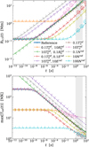 |
Fig. 7 Evolution of the width and maximum of the temperature peak after the concentrated release of energy corresponding to 1 s of a nanoflare in the solar corona. The model parameters are detailed in Sect. 5.1. The top panel shows the HWHM, while the bottom panel shows maximum temperature. The curves were calculated with Eqs. (22)–(23) and the points were calculated with simulations. Where the points are encircled ϕ∞ ≥ ϕ0, making the equations a poor approximation. The gray shaded area corresponds to t ∊ [1 s, 20 s], the time frame of interest of the simulations in Polito et al. (2018). |
6 Conclusion
In this paper, we stress that every single physics module in numerical multiphysics simulations must be tested thoroughly and separately. Many tests exist, but we found no appropriate test for Spitzer thermal conductivity in the solar atmosphere. Therefore, we derived an analytical first-order solution for nonlinear diffusivity D = KTn with any exponent n > 0 in s = {1, 2, 3) dimensions. Since the derivation and argumentation are general, the solution can easily be applied to other nonlinear diffusion problems.
The analytical solution is based on the self-similar shapes by Pattle (1959). However, where those shapes require the source quantity to diffuse in a vacuum, the new first-order solutions allow for a finite background quantity T∞. That is a key requirement for our use case, as the temperature in the solar atmosphere is nonzero. In the limit T∞ → 0+, the first-order solutions coincide with the original zeroth-order solutions. The region of validity of both the zeroth-order and first-order solutions were derived analytically and tested numerically.
We propose 4 requirements for making a benchmark based on the first-order solution: (i) The diffusing quantity ϕ0 must be large compared to the background quantity underneath it; (ii) the simulation must be run for a sufficiently long time; (iii) the width of the diffusing quantity must become large compared to the initial extent; (iv) the initial source quantity must be well-resolved numerically.
Following the requirements for making a test, we bench-marked various solvers for Spitzer conductivity in the single- and multifluid radiative MHD code Ebysus. They agree well with the first-order solutions. Going forward, Wargnier et al. (2024) will describe further the use of ROCK2 and PIROCK algorithms in the Ebysus code, while Cherry et al. (2024) will test further the solvers for Spitzer conductivity implemented in the Bifrost code.
Finally, based on the theoretically and numerically developed understanding of Spitzer conductivity, we analyzed its role during the start of a nanoflare event in the solar atmosphere. We found that conductivity alone can spread the released energy of a representative nanoflare 9 Mm in 1 s in a representative coronal atmosphere. Combining our first-order derivation with a parameter scan allow us to understand better the thermal conduction evolution in terms of the background temperature, coronal electron density, nanoflare radius, and nanoflare energy release per area perpendicular to the magnetic field. We find, as in Polito et al. (2018), that the IC before the nanoflare release impacts the thermal conduction significantly. Particularly the electron density is crucial because it is proportional to the plasma’s total heat capacity and thus inversely proportional to both the initial temperature increase and the effective temperature diffusivity K. The conduction slows down for either a larger electron density or smaller nanoflare energy release.
Acknowledgements
This research has been supported by the European Research Council through the Synergy Grant number 810218 (“The Whole Sun”, ERC-2018-SyG), from the European Union’s Horizon 2020 research and innovation programme under the Marie Skłodowska-Curie grant agreement no. 945371, and by the Research Council of Norway through its Centres of Excellence scheme, project number 262622 (Rosseland Centre for Solar Physics – RoCS). Juan Martínez-Sykora gratefully acknowledges support by NASA grants 80NSSC23K0093, 80NSSC21K0737, 80NSSC21K1684, and contracts NNG09FA40C (IRIS) and 80GSFC21C0011 (MUSE). The simulations have been run in the Pleiades cluster through the computing projects s1061, s2601, and s2967 from the High-End Computing (HEC) division of NASA. We would like to thank F. Moreno-Insertis for the positive and fruitful discussions during the Whole Sun meeting in March, 2024.
Appendix A Thermal conductivity in a plasma
The conductive part of the energy equation can be written as
 (A.1)
(A.1)
where e is the internal energy per unit volume and Fc is the heat flux vector. In a magnetized plasma, the heat flux vector can be split into two parts (see Priest 1984, p. 86)
 (A.2)
(A.2)
where κ is the thermal conduction tensor and the subscripts || and ⊥·signify components parallel and perpendicular to the magnetic field vector B, respectively. In the solar atmosphere, the perpendicular conduction is typically significantly smaller than the parallel. The parallel conduction coefficient for a fully ionized hydrogen plasma is (Spitzer 1962)
 (A.3)
(A.3)
which is close to 10−6T5/2 in the chromosphere and corona for a fully ionized hydrogen gas (Braginskii 1965; Priest 1984). This  is identical to the σ = 10−6 erg/(s cm K) in Rempel (2016).
For an ideal polytropic gas, the internal energy is related to the temperature as
 (A.4)
(A.4)
where cυ is the specific heat capacity per mass and µ the mean molecular mass. Assuming cυ to be constant and using the continuity equation, Eq. (A.1) can be written on the form
 (A.5)
(A.5)
where the RHS of the temperature evolution is split into a conductive term first and a convective term second. If we further assume a negligible perpendicular heat conduction κ⊥ ≪ κ|| and a constant, isotropic density ρ, the conductive term in Eq. (A.5) can be written on the form
 (A.6)
(A.6)
Appendix B Self-similar solutions
Here, we present a thorough derivation of the self-similar solutions to nonlinear diffusion, first described in the seminal paper by Pattle (1959), given in this paper as Eqs. (3-5). The derivation is based on a 2D-derivation by F. Moreno-Insertis (2024, priv. comm.) similar to that published in Moreno-Insertis et al. (2022).
We made the ansatz that the distribution T has the shape and boundary conditions
 (B.1)
(B.1)
 (B.2)
(B.2)
![$T[r > R(t);t] = 0.$](/articles/aa/full_html/2024/11/aa51707-24/aa51707-24-eq63.png) (B.3)
(B.3)
where m is a constant scale factor, a ≡ a(t) is a time-dependent scaling function and a0 ≡ a(t = 0). Equation (B.3) says that the distribution T is zero beyond some finite radius, giving it compact support. We can choose m so that the solution of Eq. (1) has a constant volume integral in s dimensions. The integral out to a radius rλ = λa(t), where λ is an arbitrary constant, is
 (B.4)
(B.4)
where Ωs = {2, 2π, 4π} is the total solid angle for s = {1, 2, 3} dimensions. The integral is only constant in time if m ≡ s.
Next, we inserted Eq. (B.1) with m = s into Eq. (1). By differentiating with respect to (wrt) time and space, followed by isolating all terms with explicit time dependence on the left-hand side (LHS), we ended up with
 (B.5)
(B.5)
where the apostrophe marks a partial differentiation with respect to ξ, that is f′ ≡ ∂f /∂ξ. As a consequence of the separation of variables, the RHS is independent of time, making the LHS constant in time. That is achieved when
 (B.6)
(B.6)
where χ is a constant to be determined later, proportional to the RHS of Eq. (B.5).
We inserted Eq. (B.6) into Eq. (B.5) to get
 (B.7)
(B.7)
which we integrated wrt ξ to get
 (B.8)
(B.8)
where the integration constant C1 = 0, because of the boundary condition in Eq. (B.2). We made a separation of variables by isolating f on the RHS and integrated once more to get
 (B.9)
(B.9)
where the condition f (0) = T(0, 0) ≡ T0 has been used to define an integration constant.
As we were interested in a solution that eventually would go to zero, we saw that f(r/a) had to be zero beyond a radius R(t) defined by setting Eq. (B.9) to zero
 (B.10)
which increases with time for χ > 0, as expected for diffusion. By combining the expressions for a(t)/a0 and f(r/a), we got
 (B.11)
The constant inverse time scale is defined through (B.10) as
 (B.12)
This concludes the derivation of Eqs. (3-5) in Sect. 2.1.
References
- Abdulle, A. 2002, SIAM J. Sci. Comput., 23, 2041 [CrossRef] [Google Scholar]
- Abdulle, A., & Li, T. 2008, Commun. Math. Sci., 6, 845 [CrossRef] [Google Scholar]
- Abdulle, A., & Medovikov, A. A. 2001, Numer. Math., 90, 1 [CrossRef] [Google Scholar]
- Abdulle, A., & Vilmart, G. 2013, J. Computat. Phys., 242, 869 [CrossRef] [Google Scholar]
- Abramowitz, M. & Stegun, I. A. 1965, Handbook of Mathematical Functions with Formulas, Graphs, and Mathematical Tables (New York: Dover Publications, Inc.) [Google Scholar]
- Bakke, H., Carlsson, M., Voort, L. R. v. d., et al. 2022, A&A, 659, A186 [NASA ADS] [CrossRef] [EDP Sciences] [Google Scholar]
- Braginskii, S. 1965, Rev. Plasma Phys., 1, 205 [NASA ADS] [Google Scholar]
- Cherry, G., Szydlarski, M., & Gudiksen, B. 2024, A&A, in press, https://doi.org/10.1051/0004-6361/202452012 [NASA ADS] [CrossRef] [EDP Sciences] [Google Scholar]
- Diez, J. A., Gratton, J., & Minotti, F. 1992, Q. Appl. Math., 50, 401 [CrossRef] [Google Scholar]
- Gudiksen, B. V., Carlsson, M., Hansteen, V. H., et al. 2011, A&, 531, A154 [NASA ADS] [CrossRef] [EDP Sciences] [Google Scholar]
- Kowalski, A. F., Allred, J. C., & Carlsson, M. 2024, ApJ, 969, 121 [NASA ADS] [CrossRef] [Google Scholar]
- Martínez-Sykora, J., Szydlarski, M., Hansteen, V. H., & Pontieu, B. D. 2020, ApJ, 900, 101 [CrossRef] [Google Scholar]
- Moreno-Insertis, F., Nóbrega-Siverio, D., Priest, E. R., & Hood, A. W. 2022, A&A, 662, A42 [NASA ADS] [CrossRef] [EDP Sciences] [Google Scholar]
- Parker, E. N. 1988, ApJ, 330, 474 [Google Scholar]
- Pattle, R. E. 1959, Q. J. Mech. Appl. Math., 12, 407 [CrossRef] [Google Scholar]
- Polito, V., Testa, P., Allred, J., et al. 2018, ApJ, 856, 178 [NASA ADS] [CrossRef] [Google Scholar]
- Press, W. H., Teukolsky, S. A., Vetterling, W. T., & Flannery, B. P. 2007, Numerical Recipes: The Art of Scientific Computing, 3rd edn. (Cambridge University Press) [Google Scholar]
- Priest, E. R. 1984, Solar Magnetohydrodynamics (D. Reidel Publishing Company) [Google Scholar]
- Reep, J. W., Bradshaw, S. J., & Alexander, D. 2015, ApJ, 808, 177 [NASA ADS] [CrossRef] [Google Scholar]
- Rempel, M. 2016, ApJ, 834, 10 [NASA ADS] [CrossRef] [Google Scholar]
- Sod, G. A. 1978, J. Computat. Phys., 27, 1 [CrossRef] [Google Scholar]
- Spitzer, L. 1962, Physics of Fully Ionized Gases (New York: Interscience) [Google Scholar]
- Testa, P., De Pontieu, B., Allred, J., et al. 2014, Science, 346, 1255724 [Google Scholar]
- Wargnier, Q. M., Vilbert, G., Martínez-Sykora, J., Hansteen, V. H., & De Pontieu, B. 2024, A&A, submitted [arXiv:2409.15552] [Google Scholar]
- Zbinden, C. J. 2011, SIAM J. Sci. Comput., 33, 1707 [CrossRef] [Google Scholar]
All Tables
All Figures
|
Fig. 1 Illustration of self-similar solutions in s = 1 dimensions for different n given by the legend. All solutions have peak value T0 = 1 and total quantity ϕ0 = 1, being symmetric around r = 0. |
| In the text | |
|
Fig. 2 Illustration of ICs with a background value T∞ ≥ 0 for s = 1 dimensions and n = 5/2. |
| In the text | |
|
Fig. 3 Verification of analytical derivation. Each plot shows the IC, as well as the simulation run using solve_ivp in Python, zeroth-order solution T(0), and first-order solution T(1), all at a later time such that χt >> 1. The colored ‘+’ corresponds to the HWHM point of each calculation. This is done for increasing background values T∞/T0 given by the plot titles. The simulation box extends to r = 100 R0 in (c), preventing any impacts caused by the boundary condition. |
| In the text | |
|
Fig. 4 Verification of analytical derivation for T∞/T0 = 0.01. Comparison as a function of χt for a simulation in Python (blue markers), as well as the zeroth-order (magenta curve) and first-order solutions (three green curves). In the top panel, the absolute reduction of max[TTot] and widening of HWHM (R0.5) is shown. In the following two panels, the difference to the simulation is shown for the peak temperature and width, respectively. These panels also include the evolution of ϕ∞/ϕ0 in black. The dashed vertical line marks t = 1/χ and the dotted vertical line marks t = t’ >> 1/χ, the time of the snapshot in Fig. 3b. |
| In the text | |
|
Fig. 5 Comparison between Ebysus and the first-order expression in Eqs. (22)–(23). The narrowest curve is the IC, and the following curves are given after exponentially longer time as [3 s, 6 s, 12 s, … ]. Ebysus was run with different Spitzer methods in the different panels: (a) is explicit, (b) is the wave method from Rempel (2016), and (c) is the ROCK2 method (Abdulle & Medovikov 2001). |
| In the text | |
|
Fig. 6 Error plot for the test of Ebysus presented in Fig. 5. See the description in the similar Fig. 4. Here, several y axes are linear and the error is shown relative to the first-order perturbation theory. The symmetric logarithmic error scales in the two bottom panels go from −4 × 10⁻² to 4 × 10⁻². |
| In the text | |
|
Fig. 7 Evolution of the width and maximum of the temperature peak after the concentrated release of energy corresponding to 1 s of a nanoflare in the solar corona. The model parameters are detailed in Sect. 5.1. The top panel shows the HWHM, while the bottom panel shows maximum temperature. The curves were calculated with Eqs. (22)–(23) and the points were calculated with simulations. Where the points are encircled ϕ∞ ≥ ϕ0, making the equations a poor approximation. The gray shaded area corresponds to t ∊ [1 s, 20 s], the time frame of interest of the simulations in Polito et al. (2018). |
| In the text | |
Current usage metrics show cumulative count of Article Views (full-text article views including HTML views, PDF and ePub downloads, according to the available data) and Abstracts Views on Vision4Press platform.
Data correspond to usage on the plateform after 2015. The current usage metrics is available 48-96 hours after online publication and is updated daily on week days.
Initial download of the metrics may take a while.