| Issue |
A&A
Volume 691, November 2024
|
|
|---|---|---|
| Article Number | A225 | |
| Number of page(s) | 7 | |
| Section | Stellar structure and evolution | |
| DOI | https://doi.org/10.1051/0004-6361/202451443 | |
| Published online | 15 November 2024 | |
Nonthermal GeV emission from the Nereides nebula: Confirming the nature of the supernova remnant G107.7−5.1
Escuela de Física, Universidad de Costa Rica, Montes de Oca, San José 11501-2060, Costa Rica
⋆ Corresponding author; miguel.araya@ucr.ac.cr
Received:
10
July
2024
Accepted:
20
September
2024
Context. Recently, the Nereides nebula was discovered through deep optical emission line observations and was classified as a supernova remnant (SNR) candidate, G107.7−5.1.
Aims. Since very little is known about this SNR, we have looked at several archival datasets to better understand the environment and properties of the object.
Methods. We present a detailed analysis of the gamma-ray emission detected by the Fermi Large Area Telescope in the region of the nebula. A model of the nonthermal emission is presented that allows us to derive the particle distribution responsible for the gamma rays. We also use molecular gas and atomic hydrogen observations to try to constrain the source age and distance.
Results. An extended (∼2°) GeV source coincident with the location of the nebula is found. The nonthermal emission has a hard spectrum and is detected up to ∼100 GeV, confirming the SNR nature of this object. The GeV properties of G107.7−5.1 are similar to those of other SNRs such as G150.3 + 4.5, and it likely expands in a relatively low-density medium. The Nereides nebula is one more example of a growing population of dim SNRs detected at high energies. A simple leptonic model is able to account for the gamma-ray emission. Standard SNR evolutionary models constrain the age to be in the 10 − 50 kyr range, which is consistent with estimates of the maximum particle energy obtained from GeV observations. However, more detailed observations of the source should be carried out to better understand its properties.
Key words: ISM: supernova remnants / gamma rays: general
© The Authors 2024
 Open Access article, published by EDP Sciences, under the terms of the Creative Commons Attribution License (https://creativecommons.org/licenses/by/4.0), which permits unrestricted use, distribution, and reproduction in any medium, provided the original work is properly cited.
This article is published in open access under the Subscribe to Open model. Subscribe to A&A to support open access publication.
1. Introduction
Supernova remnants (SNRs) play an important role in the interstellar medium, modifying its composition and temperature, affecting star formation activity and accelerating cosmic rays to high energies. Studying the properties of SNRs can also help us to understand the progenitors and their evolution. ∼300 Galactic SNRs are known today (Green 2019; Ferrand & Safi-Harb 2012), most of which were discovered by radio surveys. This number represents a mismatch between the expected number of SNRs in our Galaxy (see, e.g., Li et al. 1991) and the observed number. The discrepancy may be partly explained by selection effects such as the sensitivity limits of surveys.
Recently, more SNRs and SNR candidates have been discovered using X-ray and optical observations, in some cases accompanied by nonthermal gamma-ray detections (e.g., Anderson et al. 2017; Fesen et al. 2020; Gao et al. 2020; Becker et al. 2021; Churazov et al. 2021; Araya et al. 2022; Arias et al. 2022; Filipović et al. 2023; Khabibullin et al. 2023; Zhou et al. 2024; Fesen et al. 2024). In particular, new SNRs have been found at varying heights above the Galactic plane. Studying the properties of SNRs outside the Galactic plane such as G181.1 + 9.5 (Kothes et al. 2017) and G288.8 − 6.3 (Filipović et al. 2023) can help us to understand the environment and magnetic field in the outer disk and halo as well as SNR evolution in these locations (e.g., Shelton 1998).
Deep all-sky surveys such as the one carried out at GeV energies by the Large Area Telescope (LAT) on board the Fermi satellite (Atwood et al. 2009) have proven to be valuable tools in the search for SNR candidates, which often appear as extended sources. For many unidentified extended sources in the LAT catalogs, there is no known counterpart at lower energies (Abdollahi et al. 2020). They could potentially be associated with SNRs or pulsar wind nebulae and serve to confirm the SNR nature of newly found candidates at lower energies. The SNRs can produce gamma rays through the interactions of high-energy cosmic ray electrons or protons accelerated in their shocks with ambient photon fields or gas, respectively.
In this work, we investigate the properties of the recently discovered SNR G107.7−5.1 (the Nereides nebula, Fesen et al. 2024). Optical observations reveal G107.7−5.1 to be a very faint shell of filaments nearly 3 degrees in size that, together with its relatively high Galactic latitude (Fesen et al. 2024), might explain why the source has not been found in radio surveys. We confirm the SNR nature of the object with the detection of a GeV counterpart in Fermi-LAT data. This makes the Nereides nebula the 12th confirmed SNR at relatively high Galactic latitudes that has been detected by Fermi, including several radio-dim SNRs listed by Burger-Scheidlin et al. (2024).
An extended GeV source with a hard spectrum ( with Γ = 1.95 ± 0.08stat ± 0.15sys), FHES J2304.0 + 5406 was discovered by Ackermann et al. (2018) at the location of the now-known SNR G107.7−5.1. These authors propose that FHES J2304.0 + 5406 is likely associated with an SNR or a pulsar wind nebula. The morphology of this high-energy source was modeled with a Gaussian template with a 68%-containment radius of 1.58 ± 0.35stat ± 0.17sys°. In the latest incremental version of the fourth Fermi-LAT catalog (4FGL-DR4, Ballet et al. 2023), the corresponding source is labeled 4FGL J2304.0 + 5406e, and has the same morphology as FHES J2304.0 + 5406 and a spectrum described by a log-parabola,
  , where α = 1.72 ± 0.08, β = 0.08 ± 0.04, and Eb is a fixed scale parameter. The significance of “spectral curvature” (i.e., the deviation of the source spectrum from a simple power law), however, is reported to be at the 2.6σ level.
2. Data
2.1. Fermi-LAT observations
We downloaded LAT Pass 8 observations1 from the beginning of the mission, August 2008, to March 2024, containing events reconstructed within 25° of the coordinates RA = 346.0°, Dec = 54.6° in the energy range 0.1–500 GeV. Front and back-converted SOURCE class events were used for the analysis (evclass = 128, evtype = 3), which was done with the software fermitools version 2.2.02 through the fermipy package version 1.2.0 (Wood et al. 2017). We binned the data with a spatial scale of 0.05° per pixel and ten bins in energy for exposure calculations. The analysis used the publicly available response functions appropriate for the dataset, P8R3_SOURCE_V3.
The data analysis relied on the maximum likelihood technique (Mattox et al. 1996). For a given spectral and morphological model of a source, its emission was convolved with the response functions to predict the number of counts in the spatial and energy bins. A fit of the free parameters was carried out to maximize the probability of the model explaining the data in each bin. The detection significance of a new source having one additional free parameter, for example, can be calculated as the square root of the test statistic (TS), defined as TS = − 2 log (ℒ0/ℒ), with ℒ and ℒ0 the maximum likelihood functions for a model with the new source and for the model without this additional source (the null hypothesis), respectively. In all of the models, the diffuse Galactic emission is described by the file gll_iem_v07.fits, and the isotropic emission and residual cosmic-ray background is given by iso_P8R3_SOURCE_V3_v1.txt, which are provided by fermitools. As was recommended by the LAT team, the energy dispersion correction was applied to all sources except for the isotropic component.
2.1.1. Morphology of the GeV emission
We first carried out a morphological analysis of the gamma-ray emission in the region of G107.7−5.1. For this purpose, we took advantage of the improved resolution at higher energies and only used events with energies above 10 GeV. To avoid gamma-ray contamination from cosmic-ray interactions in the Earth’s atmosphere, we set a maximum event zenith angle of 105° (Abdollahi et al. 2020). In this step, we used a region of interest with a radius of 15° around RA = 346.0°, Dec = 54.6° and included in the model the cataloged sources from 4FGL-DR4 found within 20° of the center. To optimize the model, initially we carried out a preliminary fit of the spectral normalizations of the 4FGL-DR4 sources located within 10° of the center, as well as the spectral indices and normalizations of the sources located within 5° of the center of the region. We set the normalizations of the diffuse components to be free in all fits.
We searched for potentially new point sources in the region to improve the model of the background using the fermipy function find_sources. This algorithm searches for peaks in the TS map obtained when subtracting the cataloged sources. In this case, we only set free the normalizations of the model sources found within 3° from the center. We added new source candidates to the model if their calculated  was above a threshold of 4. The spectral function used for the point sources was a simple power law. After adding the new candidate sources to the model, we set the parameters of the sources to be free as before (the source normalizations for sources within 10° of the center, and the spectral indices and normalizations for sources within 5° of the center) and performed a new fit.
We compared two alternative models for the emission from G107.7−5.1: the 2D Gaussian template used in the 4FGL-DR4 catalog and a uniform 2D disk. After removing the source 4FGL J2304.0 + 5406e from the model, we searched for the disk radius (r) and center location that maximize the likelihood (again with only the normalizations of the model sources located within 3° from the center free to vary) of resulting in the values r = 1.02 ± 0.03°, RA = 346.14 ± 0.04°, and Dec = 54.31 ± 0.05° (1σ statistical uncertainties quoted).
After freeing the background sources again, in the manner explained before, we performed two independent fits using the disk and Gaussian templates, assuming simple power laws for the spectral shape with a free index and normalization. The fit using the disk results in a slightly higher likelihood value, with TS = 72.5, compared to the fit with the Gaussian, which gives TS = 68.2. We thus adopted the disk template to model the GeV emission from the SNR and used the Gaussian morphology to estimate systematic errors in the spectral parameters resulting from changing the morphology (see below).
In order to obtain a map of the GeV emission with improved statistics, the procedure described above for optimizing the model was repeated for events with energies above 2 GeV. Our model provides a satisfactory fit to the background sources (see Appendix A). The best-fit disk found in this section was removed from the model and a TS map was calculated by optimizing the spectral normalization of a putative point source that was moved in a grid of positions, and calculating its TS in each fit. We used a spectrum described by a power law for the point source with a fixed index of 2. Fig. 1 shows the resulting TS map. The extension and location of the best-fit GeV disk is shown in the figure as well as the center location of the 4FGL Gaussian model and the locations of background 4FGL-DR4 sources. Our disk model matches the location of the SNR shell, while using the catalogued source 4FGL J2304.0 + 5406e does not improve the fit, and this source is more extended than the SNR. The extension of this source was determined by Ackermann et al. (2018) using events in the energy range of 1 GeV–1 TeV, while we used events above 10 GeV that have a much better resolution.
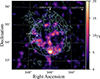 |
Fig. 1. TS map for events with energies above 2 GeV showing the emission from G107.7−5.1. The circle represents the uniform disk obtained in this work to model the morphology of the gamma-ray emission. The contours show the optical emission of the SNR shell taken from Fesen et al. (2024). The marks + and × indicate the center locations of the disk and the extended 4FGL source, respectively, while the boxes show the locations of the other 4FGL-DR4 sources in the region. |
The point source 4FGL J2309.0 + 5425 is seen in the direction of the shell of the SNR and according to Ballet et al. (2023) could be related to the X-ray source 1RXS J230852.2 + 542559. The source 4FGL J2303.9 + 5554 is seen just north of the SNR shell and is classified as a blazar candidate by Kerby et al. (2021). Both of these sources are clearly point-like in LAT data, and thus likely unrelated to the shell emission (see Appendix B); therefore, they were kept in the background model. Fig. 1 also shows contours from the optical [O III] emission of the SNR, obtained from Fesen et al. (2024). [O III] emission is associated with ionization, resulting for example from high-velocity shocks, and can be used to trace the remnant’s actual morphology. A consistency is seen between the extension and location of the gamma-ray emission and the SNR.
2.1.2. Gamma-ray spectrum
We collected all events in the energy range of 0.1–500 GeV to study the high-energy spectrum of G107.7−5.1. We used similar filtering parameters as in the previous section except for the maximum zenith angle, which was set to 90°. To account for the larger point spread function of low-energy events, we also increased the radius of the region of interest to 20° and added cataloged sources located up to a distance of 25° from the center of the region. We modeled the SNR using the disk obtained in the previous section and searched for new point source candidates to improve the background model (see Appendix A). After optimizing the spectral parameters of sources following the procedure of the previous section, we produced a spectral energy distribution (SED) of G107.7−5.1 dividing the data into 11 energy bins equally spaced on a logarithmic scale. In each bin, the spectrum of the SNR was modeled using a power law with a fixed spectral index of the form  and the normalization, N0, was fit. We did not significantly detect the source in any bin below ∼1 GeV or above ∼100 GeV and derived 95%-confidence level upper limits for those bins, as can be seen in Table 1.
SED measurements of SNR G107.7−5.1.
With the goal of constraining the spectral shape of the SNR, we compared two fits in the energy range of 0.1–500 GeV using a simple power law and a log-parabola. The log-parabola resulted in a better fit to the data, with a difference in TS values of Δ TS = 23. For an additional degree of freedom in the model, this corresponds to an improvement at the 4.8σ level, which demonstrates that the source spectrum is significantly curved. This is consistent with the results shown in the 4FGL catalog for the source 4FGL J2304.0 + 5406e, where its spectrum is modeled with a log-parabola, although the reported significance of curvature is lower. Adopting the morphology of the 4FGL catalog (2D Gaussian), however, does not provide an improvement in the fit, resulting in TS = 100.3, compared to TS = 98.8 obtained with the disk template found in the previous section. This result is consistent with the morphological study in this work.
A fit to the spectral function  in the energy range of 0.1–500 GeV produced the values
  MeV−1 s−1 cm−2, α = 1.67 ± 0.01 ± 0.12, and
  (the first errors are statistical, while the second are systematic) for a fixed parameter, Eb = 13 GeV. We considered two factors that affect the source modeling to estimate the systematic errors in the parameters, the source morphology, and the uncertainty in the effective area of the LAT. For the first, we calculated the difference between parameter values obtained using the 2D Gaussian template from the 4FGL catalog and those found with the disk template. For the second effect, we used a set of bracketing response functions following Ackermann et al. (2012), fixing the value of the pivot energy at Eb = 13 GeV for which the propagated error in the differential flux was minimal, to estimate the differences in the parameters obtained using the alternative and the nominal effective area models. For the combined systematic uncertainty, we added the errors from both effects in quadrature. The cause of the large error in the spectral normalization, N0, is the alternative Gaussian template, which predicts about twice the flux for the source. The gamma-ray energy flux of the source integrated above 1 GeV is ∼5.8 × 10⁻⁶ MeV cm−2 s−1, corresponding to a luminosity of ∼1.1 × 1033 dkpc2 erg s−1, where dkpc is the source distance in kiloparsecs.
2.2. GeV emission model
Nonthermal emission in SNRs can be produced by the relativistic particles accelerated at the shock. High-energy electrons are responsible for the synchrotron emission in the radio that is characteristic of many SNRs. These same electrons can produce gamma rays through inverse Compton (IC) scattering of low-energy ambient photons, or through bremsstrahlung emission resulting from interactions with ambient nuclei if the densities are high enough. These mechanisms are thus leptonic. In the hadronic scenario, the high-energy nuclei can produce π mesons in collisions with ambient matter if the density is high enough. The resulting neutral pions decay into gamma rays that can be detected. They are usually observed in regions where SNRs interact with molecular clouds.
The rotational J = 1 − 0 transition of the carbon monoxide molecule has been widely used as a tracer of molecular hydrogen in astronomy. We downloaded data from the CO survey by Dame et al. (2001) (individual survey DHT18) to look for emission line signals in the direction of G107.7−5.1. No significant emission is apparent at any velocities, and Fig. 2 shows the integrated emission in a region of the sky around the location of the SNR.
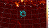 |
Fig. 2. Velocity-integrated CO (J = 1 − 0) emission line from Dame et al. (2001) with the optical contours of the SNR overlaid (cyan, same as Fig. 1). Map units are K km s−1 and grid coordinates are RA and Dec (°). |
Although more detailed observations should be carried out, it is possible as these data suggest that G107.7−5.1 is evolving in a low-density environment (see Section 3 for an estimate of the ambient densities). This seems reasonable given the location of the SNR 5° below the Galactic plane. In fact, as is shown in Fig. 1, the gamma-ray emission is more prominent in the south of the SNR, which is the region that is farthest from the Galactic plane.
We applied a simple one-zone leptonic model to account for the GeV flux from G107.7−5.1, to constrain the parameters of the particle distribution responsible for the emission. Given the likely low-density environment of the SNR, we did not consider a hadronic origin. We compared two functions for the underlying lepton distribution, a simple power law (PL) of the form  , and a power law with an exponential cutoff (EC),
  , where Ee is the electron energy, s and Ec are the spectral index and energy cutoff, respectively, and a is the normalization. We fit the observed fluxes from Table 1 with an inverse Compton model using the NAIMA package (Zabalza 2015). The IC calculations were implemented from Khangulyan et al. (2014).
For the seed photon fields, we included the cosmic microwave background radiation (CMB) and the local far-infrared (FIR) and optical (NIR) fields. While the first was modeled as a black body, the other two were modeled as black bodies with a dilution factor, and had densities and temperatures of 0.2 eV cm−3 and 30 K in the FIR, and 0.3 eV cm−3 and 3000 K in the NIR. These values were estimated by Tibaldo et al. (2018) using a model from Popescu et al. (2017). Comparing the Bayesian information criterion (BIC) from the fits, we obtained BICPL − BICEC = 2.07, and thus the particle distribution that has an exponential cutoff is a better model.
Although with the observations analyzed in this work we cannot constrain the synchrotron flux level from the source, modeling the GeV observations under the IC scenario allows us to determine the present particle slope and cutoff energy. However, future observations, particularly at the highest energies, should be carried out to better constrain Ec. The resulting values are  and
and  TeV, respectively. Assuming a source distance of 1 kpc, the total energy required in the particles is 8.6 × 1046 erg. If we fit the GeV spectrum with a particle distribution in the form of a broken power law, the values obtained for the spectral indices before and after the break are
  ,
,  , respectively, with a break energy of
  TeV; however, the fit does not represent an improvement with respect to the more simple exponential cutoff model, with an increase of ∼3.5 in the value of the BIC. Fig. 3 shows the GeV data from G107.7−5.1 and the leptonic model described in this section.
 |
Fig. 3. Simple one-zone leptonic model for the nonthermal GeV emission from G107.7−5.1 analyzed in this work. |
3. Discussion
The gamma-ray emission presented in this work shows a morphology that is consistent with that of the newly discovered SNR candidate G107.7−5.1 (the Nereides nebula), which we argue confirms the SNR nature of the object. It becomes a new example of an SNR at relatively high Galactic latitudes that is detected at GeV energies. Besides the seven objects listed by Burger-Scheidlin et al. (2024), other examples could include the Cygnus Loop, HB 21 (G89.0 + 4.7), G332.5 − 5.6, and the remnant of Kepler’s supernova (Katagiri et al. 2011; Pivato et al. 2013; Xiang & Jiang 2021; Luo et al. 2024).
The spectral slope measured for G107.7−5.1 is hard (α ∼ 1.67). A softer spectral index was recently found for the Ancora SNR (G288.8 − 6.3 with α ∼ 2.3, Burger-Scheidlin et al. 2024), which might indicate that G107.7−5.1 is in a younger evolutionary stage. Examples of SNRs with a spectral slope at GeV energies similar to that of G107.7−5.1 are Calvera’s SNR and G150.3 + 4.5 (Araya 2023; Devin et al. 2020). Both are radio-dim SNRs that likely expand in low-density environments, which could also be the case for the Nereides nebula. We note the GeV similarities between G107.7−5.1 and G150.3 + 4.5. Their photon spectral indices are very similar, and Devin et al. (2020) also found similar maximum electron energies of ∼5 TeV in a leptonic (IC) scenario for the gamma rays.
As we showed in Section 2.2, no molecular gas is seen in the region of the SNR. The WISE catalog of HII regions (Anderson et al. 2014) likewise shows no object close to the SNR. This would explain the low GeV luminosity of G107.7−5.1, ∼1033 erg s−1 (assuming a distance of 1 kpc) compared to those of SNRs interacting with molecular clouds (e.g., Acero et al. 2016).
We have shown a simple leptonic model that accounts for the GeV fluxes of the Nereides nebula. Although the particle spectral index of 2 found in the model is expected for a diffusive shock-accelerated electron spectrum, a relevant feature in the spectrum is its curvature, similar to that of G150.3 + 4.5 (Devin et al. 2020). This could naturally be explained by the cooling of the electrons responsible for the emission, which results in a spectral break. However, the estimated cooling times are relatively large. Assuming that electrons cool due to synchrotron and IC-CMB losses and that this causes the observed particle spectral turnover at ∼4 TeV, an age estimate can be obtained by calculating the corresponding cooling time as (Aharonian et al. 2006),
with Bμ the magnetic field in units of μG. Using Bμ = 3, the age is 160 kyr, which is not reasonable for an SNR with a well-defined shell. On the other hand, for an average field value, Bμ > 10, the corresponding age is < 28 kyr. We note that these estimates should be taken cautiously, since the magnetic field is a function of time and was likely larger in the past, making the particles cool faster. Future detailed observations in the radio and above ∼100 GeV should confirm or rule out a spectral break and better constrain any spectral turnover.
We estimated the SNR age from the ambient parameters. From optical observations, an angular radius of ∼1.2° is determined for the SNR shell. The physical sizes of SNRs with well-defined shells rarely exceed 100 pc (e.g., Badenes et al. 2010). Thus, the distance to G107.7−5.1 is likely to be d < 2.4 kpc. Using a column density calculator, employing the method by Willingale et al. (2013),3 we found that the atomic hydrogen contribution dominates over that of molecular hydrogen in the direction of the SNR. With data from the HI4PI atomic hydrogen survey (HI4PI Collaboration et al. 2016, spectral resolution ∼1.49 km s−1), we chose four ∼5 km s−1-wide local standard of rest velocity (vlsr) intervals and, assuming that the measured velocities arise from the differential Galactic rotation of the gas, we calculated the associated kinematic distances using the Galactic rotation model from Brand & Blitz (1993). We only selected velocities consistent with the constraint d < 2.4 kpc. Given the location of the SNR beyond the solar orbit, a value of vlsr uniquely determines the kinematic distance. In each velocity interval, we integrated the brightness temperature of the atomic emission and estimated the column density (NH) in the direction of the SNR in the optically thin limit (see, e.g., Dickey & Benson 1982). With an integration line-of-sight length of ∼0.5 kpc for each interval and the average value of NH, we estimated the atomic number density (n) of the interstellar medium. Finally, using the Sedov-Taylor (ST) solution, we calculated the SNR age (tST) from its radius (RSNR) and the ambient density, assuming an initial kinetic energy in the SNR of 1051 erg (note that for the densities obtained here the SNR is predicted to still be in the ST stage, see Cioffi et al. 1988). The results are shown in Table 2. The SNR age is constrained in the 10 − 50 kyr range under the assumption that the ST solution applies. For the different values of the SNR radii and ages, we also estimated the ST shock speed ( ), which is shown in Table 2.
SNR parameters.
If the downstream magnetic field in the SNR has a similar value to that found for G150.3 + 4.5 (∼5 μG), the cooling time is ∼87 kyr, which is larger than the ST age. In this case, no break is expected in the particle distribution and a spectral turnover appears, since the acceleration timescale is limited by the source age, tacc ≈ tST. The acceleration timescale is inversely proportional to the magnetic field and the square of the shock speed, and proportional to the maximum particle energy (here equal to 4 TeV) and the ratio between the mean free path and the gyroradius (Parizot et al. 2006), k. For evolved SNRs, we expect that k > 1. Adopting a shock compression ratio, r = 4, and the values of vsh with their corresponding ages tST = 52, 48, 28, 10 kyr from Table 2, we obtain k = 177, 215, 87, 12, respectively, which are plausible values. These estimates, however, assume a constant shock speed, which is a considerable simplification.
If, on the other hand, the maximum electron energy observed for this source is the result of the balance of synchrotron losses and acceleration in a slow shock, the condition τcool ≈ tacc < tST can be accomplished for the four cases, tST = 52, 48, 28, 10 kyr, if k ≲ 3.6 with B ≳ 7 μG, k ≲ 2.6 with B ≳ 7.3 μG, k ≲ 3 with B ≳ 10 μG, and k ≲ 4.8 with B ≳ 17 μG, respectively. These values for the parameters are also reasonable, making this scenario possible too. In summary, the estimated ST ages are consistent with the GeV spectrum of G107.7−5.1.
Finally, although we note that the kinematic distance determination likely suffers from high uncertainties (Wenger et al. 2018) and the SNR parameters derived here should be taken cautiously, it seems likely that G107.7−5.1 is one more example in a population consisting of relatively evolved and dim SNRs detected at GeV energies, possibly evolving in low-density environments, and for which a leptonic scenario is a reasonable explanation for the origin of the gamma rays. The existence of such a population has been proposed before (Araya 2020) and some examples of similar objects are given by Araya (2023). Future, more detailed observations of the Nereides nebula should be carried out to better constrain the source properties and contribute to the understanding of SNR evolution.
Acknowledgments
We thank Robert A. Fesen for providing us with the optical image of SNR G107.7−5.1 and the anonymous referee for comments and suggestions that helped improve the quality of this work. We thank funding from Universidad de Costa Rica under grant number C4228.
References
- Abdollahi, S., Acero, F., Ackermann, M., et al. 2020, ApJS, 247, 33 [Google Scholar]
- Acero, F., Ackermann, M., Ajello, M., et al. 2016, ApJS, 224, 8 [NASA ADS] [CrossRef] [Google Scholar]
- Ackermann, M., Ajello, M., Albert, A., et al. 2012, ApJS, 203, 4 [Google Scholar]
- Ackermann, M., Ajello, M., Baldini, L., et al. 2018, ApJS, 237, 32 [NASA ADS] [CrossRef] [Google Scholar]
- Aharonian, F., Akhperjanian, A. G., Bazer-Bachi, A. R., et al. 2006, A&A, 460, 365 [NASA ADS] [CrossRef] [EDP Sciences] [Google Scholar]
- Anderson, L. D., Bania, T. M., Balser, D. S., et al. 2014, ApJS, 212, 1 [Google Scholar]
- Anderson, L. D., Wang, Y., Bihr, S., et al. 2017, A&A, 605, A58 [NASA ADS] [CrossRef] [EDP Sciences] [Google Scholar]
- Araya, M. 2020, MNRAS, 492, 5980 [NASA ADS] [CrossRef] [Google Scholar]
- Araya, M. 2023, MNRAS, 518, 4132 [Google Scholar]
- Araya, M., Hurley-Walker, N., & Quirós-Araya, S. 2022, MNRAS, 510, 2920 [NASA ADS] [CrossRef] [Google Scholar]
- Arias, M., Botteon, A., Bassa, C. G., et al. 2022, A&A, 667, A71 [NASA ADS] [CrossRef] [EDP Sciences] [Google Scholar]
- Atwood, W. B., Abdo, A. A., Ackermann, M., et al. 2009, ApJ, 697, 1071 [CrossRef] [Google Scholar]
- Badenes, C., Maoz, D., & Draine, B. T. 2010, MNRAS, 407, 1301 [NASA ADS] [CrossRef] [Google Scholar]
- Ballet, J., et al. (The Fermi-LAT collaboration) 2023, ArXiv e-prints [arXiv:2307.12546] [Google Scholar]
- Becker, W., Hurley-Walker, N., Weinberger, C., et al. 2021, A&A, 648, A30 [NASA ADS] [CrossRef] [EDP Sciences] [Google Scholar]
- Brand, J., & Blitz, L. 1993, A&A, 275, 67 [NASA ADS] [Google Scholar]
- Burger-Scheidlin, C., Brose, R., Mackey, J., et al. 2024, A&A, 684, A150 [NASA ADS] [CrossRef] [EDP Sciences] [Google Scholar]
- Churazov, E. M., Khabibullin, I. I., Bykov, A. M., et al. 2021, MNRAS, 507, 971 [NASA ADS] [CrossRef] [Google Scholar]
- Cioffi, D. F., McKee, C. F., & Bertschinger, E. 1988, ApJ, 334, 252 [Google Scholar]
- Dame, T. M., Hartmann, D., & Thaddeus, P. 2001, ApJ, 547, 792 [Google Scholar]
- Devin, J., Lemoine-Goumard, M., Grondin, M. H., et al. 2020, A&A, 643, A28 [NASA ADS] [CrossRef] [EDP Sciences] [Google Scholar]
- Dickey, J. M., & Benson, J. M. 1982, AJ, 87, 278 [NASA ADS] [CrossRef] [Google Scholar]
- Ferrand, G., & Safi-Harb, S. 2012, Adv. Space Res., 49, 1313 [Google Scholar]
- Fesen, R. A., Weil, K. E., Raymond, J. C., et al. 2020, MNRAS, 498, 5194 [NASA ADS] [CrossRef] [Google Scholar]
- Fesen, R. A., Drechsler, M., Strottner, X., et al. 2024, ApJS, 272, 36 [NASA ADS] [CrossRef] [Google Scholar]
- Filipović, M. D., Dai, S., Arbutina, B., et al. 2023, AJ, 166, 149 [CrossRef] [Google Scholar]
- Gao, X. Y., Reich, P., Reich, W., Hou, L. G., & Han, J. L. 2020, MNRAS, 493, 2188 [NASA ADS] [CrossRef] [Google Scholar]
- Green, D. A. 2019, J. Astrophys. Astron., 40, 36 [Google Scholar]
- HI4PI Collaboration (Ben Bekhti, N., et al.) 2016, A&A, 594, A116 [NASA ADS] [CrossRef] [EDP Sciences] [Google Scholar]
- Katagiri, H., Tibaldo, L., Ballet, J., et al. 2011, ApJ, 741, 44 [NASA ADS] [CrossRef] [Google Scholar]
- Kerby, S., Kaur, A., Falcone, A. D., et al. 2021, ApJ, 923, 75 [NASA ADS] [CrossRef] [Google Scholar]
- Khabibullin, I. I., Churazov, E. M., Bykov, A. M., Chugai, N. N., & Sunyaev, R. A. 2023, MNRAS, 521, 5536 [NASA ADS] [CrossRef] [Google Scholar]
- Khangulyan, D., Aharonian, F. A., & Kelner, S. R. 2014, ApJ, 783, 100 [Google Scholar]
- Kothes, R., Reich, P., Foster, T. J., & Reich, W. 2017, A&A, 597, A116 [NASA ADS] [CrossRef] [EDP Sciences] [Google Scholar]
- Li, Z., Wheeler, J. C., Bash, F. N., & Jefferys, W. H. 1991, ApJ, 378, 93 [Google Scholar]
- Luo, M.-H., Tang, Q.-W., & Mo, X.-R. 2024, Res. Astron. Astrophys., 24, 045012 [CrossRef] [Google Scholar]
- Mattox, J. R., Bertsch, D. L., Chiang, J., et al. 1996, ApJ, 461, 396 [Google Scholar]
- Parizot, E., Marcowith, A., Ballet, J., & Gallant, Y. A. 2006, A&A, 453, 387 [NASA ADS] [CrossRef] [EDP Sciences] [Google Scholar]
- Pivato, G., Hewitt, J. W., Tibaldo, L., et al. 2013, ApJ, 779, 179 [NASA ADS] [CrossRef] [Google Scholar]
- Popescu, C. C., Yang, R., Tuffs, R. J., et al. 2017, MNRAS, 470, 2539 [NASA ADS] [CrossRef] [Google Scholar]
- Shelton, R. L. 1998, ApJ, 504, 785 [NASA ADS] [CrossRef] [Google Scholar]
- Tibaldo, L., Zanin, R., Faggioli, G., et al. 2018, A&A, 617, A78 [NASA ADS] [CrossRef] [EDP Sciences] [Google Scholar]
- Wenger, T. V., Balser, D. S., Anderson, L. D., & Bania, T. M. 2018, ApJ, 856, 52 [Google Scholar]
- Willingale, R., Starling, R. L. C., Beardmore, A. P., Tanvir, N. R., & O’Brien, P. T. 2013, MNRAS, 431, 394 [Google Scholar]
- Wood, M., Caputo, R., Charles, E., et al. 2017, Int. Cosmic R. Conf., 301, 824 [NASA ADS] [CrossRef] [Google Scholar]
- Xiang, Y., & Jiang, Z. 2021, ApJ, 908, 22 [NASA ADS] [CrossRef] [Google Scholar]
- Zabalza, V. 2015, Proc. of Int. Cosmic R. Conf., 2015, 922 [NASA ADS] [Google Scholar]
- Zhou, X., Su, Y., Yang, J., Chen, Y., & Jiang, Z. 2024, A&A, 683, A107 [NASA ADS] [CrossRef] [EDP Sciences] [Google Scholar]
Appendix A: Residual TS maps
This section presents residual TS maps of a 15° ×15°-region around the location of G107.7−5.1 obtained after subtracting all the background sources as well as the emission from the SNR. Fig. A.1 shows the maps for events with energies above 100 MeV and for events with energies above 2 GeV. The positions of the catalogued 4FGL sources and the new point sources added to the model during the optimization step are shown. The locations of the new point sources found above 2 GeV generally correspond with sources found at lower energies. However, more sources are found at lower energies, particularly towards the north of the SNR where the Galactic plane is located.
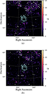 |
Fig. A.1. Residual TS maps obtained after subtracting all the background 4FGL sources (squares), additional excess emission modeled as point sources in this work (circles) and the SNR G107.7−5.1, in two analysis intervals: 0.1–500 GeV (a) and 2–500 GeV (b). The contours represent the optical emission from the SNR shell. |
Appendix B: On the background sources 4FGL J2309.0 + 5425 and 4FGL J2303.9 + 5554
Fig. B.1 is a TS map obtained with events having energies above 10 GeV showing the SNR emission as well as that of 4FGL J2309.0 + 5425 and 4FGL J2303.9 + 5554. The image clearly shows that these sources are point-like for the LAT and thus possibly associated to independent objects and not the shell of the SNR. As indicated previously, 4FGL J2309.0 + 5425, seen in the eastern side of the SNR, is believed to be associated with an X-ray source, while 4FGL J2303.9 + 5554, seen to the north was classified as a likely blazar by Kerby et al. (2021).
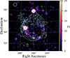 |
Fig. B.1. A TS map above 10 GeV obtained after removing the SNR and the sources 4FGL J2309.0 + 5425 and 4FGL J2303.9 + 5554 from the model (thus causing them to appear in the map). The large circle indicates the gamma-ray disk model for the SNR (whose optical contours are shown) and the squares are the catalogued positions of the 4FGL sources. The upper-left circle indicates the 68%-containment region of the LAT point spread function for both front- and back-converted events at 10 GeV. |
All Tables
All Figures
|
Fig. 1. TS map for events with energies above 2 GeV showing the emission from G107.7−5.1. The circle represents the uniform disk obtained in this work to model the morphology of the gamma-ray emission. The contours show the optical emission of the SNR shell taken from Fesen et al. (2024). The marks + and × indicate the center locations of the disk and the extended 4FGL source, respectively, while the boxes show the locations of the other 4FGL-DR4 sources in the region. |
| In the text | |
|
Fig. 2. Velocity-integrated CO (J = 1 − 0) emission line from Dame et al. (2001) with the optical contours of the SNR overlaid (cyan, same as Fig. 1). Map units are K km s−1 and grid coordinates are RA and Dec (°). |
| In the text | |
|
Fig. 3. Simple one-zone leptonic model for the nonthermal GeV emission from G107.7−5.1 analyzed in this work. |
| In the text | |
|
Fig. A.1. Residual TS maps obtained after subtracting all the background 4FGL sources (squares), additional excess emission modeled as point sources in this work (circles) and the SNR G107.7−5.1, in two analysis intervals: 0.1–500 GeV (a) and 2–500 GeV (b). The contours represent the optical emission from the SNR shell. |
| In the text | |
|
Fig. B.1. A TS map above 10 GeV obtained after removing the SNR and the sources 4FGL J2309.0 + 5425 and 4FGL J2303.9 + 5554 from the model (thus causing them to appear in the map). The large circle indicates the gamma-ray disk model for the SNR (whose optical contours are shown) and the squares are the catalogued positions of the 4FGL sources. The upper-left circle indicates the 68%-containment region of the LAT point spread function for both front- and back-converted events at 10 GeV. |
| In the text | |
Current usage metrics show cumulative count of Article Views (full-text article views including HTML views, PDF and ePub downloads, according to the available data) and Abstracts Views on Vision4Press platform.
Data correspond to usage on the plateform after 2015. The current usage metrics is available 48-96 hours after online publication and is updated daily on week days.
Initial download of the metrics may take a while.