| Issue |
A&A
Volume 694, February 2025
|
|
|---|---|---|
| Article Number | A211 | |
| Number of page(s) | 8 | |
| Section | The Sun and the Heliosphere | |
| DOI | https://doi.org/10.1051/0004-6361/202451436 | |
| Published online | 14 February 2025 | |
Dynamics of energetic electrons scattered in the solar wind
Magnetohydrodynamics and test-particle simulations
LESIA, Observatoire de Paris, Université PSL, CNRS, Sorbonne Université, Université Paris Cité, 5 place Jules Janssen, 92195 Meudon, France
⋆ Corresponding author; ahmed.houeibib@obspm.fr
Received:
9
July
2024
Accepted:
20
December
2024
We model the transport of solar energetic particles (SEPs) in the solar wind. We propagated relativistic test particles in the field of a steady three-dimensional magnetohydrodynamic simulation of the solar wind. We used the code MPI-AMRVAC for the wind simulations and integrated the relativistic guiding center equations using a new third-order-accurate predictor-corrector time-integration scheme. Turbulence-induced scattering of the particle trajectories in velocity space was taken into account through the inclusion of a constant field-aligned scattering mean free path λ∥. We considered mid-range SEP electrons of 81 keV injected into the solar wind at a heliocentric distance of 0.28 AU and a magnetic latitude of 24°. For λ∥ = 0.5 AU, the simulated velocity pitch angle distributions agree qualitatively well with in situ measurements at 1 AU. More generally, for λ∥ in the range 0.1–1 AU, an energy-loss rate associated with the velocity drift of about 10% per day is observed. The energy loss is attributable to the magnetic curvature and gradient-induced poleward drifts of the electrons against the dominant component of the electric field. In our case study, which is representative of the average solar wind conditions, the observed drift-induced energy-loss rate is fastest near a heliocentric distance of 1.2 AU. We emphasize that adiabatic cooling is the dominant mechanism during the first 1.5 hours of propagation. Only at later times does the drift-associated loss rate become dominant.
Key words: acceleration of particles / magnetohydrodynamics (MHD) / methods: numerical / solar wind
© The Authors 2025
 Open Access article, published by EDP Sciences, under the terms of the Creative Commons Attribution License (https://creativecommons.org/licenses/by/4.0), which permits unrestricted use, distribution, and reproduction in any medium, provided the original work is properly cited.
This article is published in open access under the Subscribe to Open model. Subscribe to A&A to support open access publication.
1. Introduction
Solar energetic particles (SEPs) have attracted attention since Forbush (1946) first imputed the sporadic increase in the cosmic-ray flux measured in ionization chambers to GeV protons ejected by the Sun during flares (see Cliver et al. 2009 for more details). In the same epoch, radio astronomers started to detect flare-associated radio bursts in the frequency range < 100 MHz (Payne-Scott et al. 1947). Some of these, in particular, the type II and type III bursts (see Wild & McCready (1950)), were later suggested to be produced by a plasma instability excited by a stream of fast particles (Ginzburg & Zhelezniakov 1958). By the beginning of the 1960s (see Wild et al. 1963), it was generally accepted that radio bursts are due to the interaction of energetic particles with interplanetary plasma. These particles are accelerated either impulsively at the sites of magnetic reconnection in the solar corona or gradually, at the shock ahead of a coronal mass ejection (CME) (Reames 1999; Desai & Giacalone 2016; Klein & Dalla 2017).
After it was established that solar flares and CMEs can accelerate ions and electrons to relativistic energies, the question of their propagation throughout the turbulent heliospheric plasma arose. To model this propagation, two approaches were attempted so far. The first approach is to consider that the particle diffusion is a Markovian process that is conveniently described by the Fokker-Planck equation, which describes the propagation and the diffusion in phase-space of an initial probability distribution of particles (Parker 1965). The linearity of the Fokker-Planck equation enables analytic solutions in some simple cases, such as the case of the diffusion of energetic particles in a constant and nonmagnetized solar wind (see Parker 1965). However, for more realistic wind models, the Fokker-Planck equation has to be solved numerically on a five-dimensional grid spanning three spatial and two velocity dimensions in phase space, which can be computationally very costly (e.g., Wijsen et al. 2020, 2022). The computational costs can be reduced by integrating the trajectory of N test particles on a three-dimensional spatial grid with prescribed electric and magnetic fields. The second approach consists of computing the trajectory of a large number of individual particles in a prescribed electromagnetic field. Scattering is then modeled by hard-sphere-type collisions given a prescribed collisional mean-free path λ along the magnetic field of the particle guiding center and a post-collision angular distribution law. We follow the second approach here. Our treatment is similar to but different from the one adopted by Marsh et al. (2013), Dalla et al. (2013, 2015), where the scattering events were Poisson distributed in time with an average scattering time λ/v, that is, the average time interval between successive scattering events is constant instead of the distance of the scattering centers along the field line. The underlying physical model differs from the classical quasi-linear Fokker-Planck model, which rests on the assumption that particles change their trajectory through a succession of small-angle deviations and on the assumption of quasi-isotropy of the velocity distribution function (see e.g. Jokipii 1966, 1968; Hasselmann & Wibberenz 1968; Schlickeiser 1989). The differences can be reduced by increasing the number of test particles N and decreasing the Knudsen number λ/LB (LB is the spatial scale of the variation in the magnetic field) and provided that the adopted post-collision angular distribution law drives the velocity distribution toward isotropy (see Sect. 2.3).
We considered the propagation of electrons as test particles in the electromagnetic field of a steady-state solar wind from a 3D magnetohydrodynamic (MHD) simulation, which conveniently describes the large scales. We considered solar energetic electrons of 81 keV, which are in the mid-range for SEP electrons (see Fig. 1 in Dröge et al. (2018)). For an 81 keV electron in a magnetic field B = 1 nT, the Larmor radius is rL = 678 km (2400 km for 1 MeV electrons). This is much smaller than the order AU scales of the MHD simulation, so that we consistently integrated the equations of motion in the relativistic guiding-center approximation (GCA). The structure of the GCA equations is far more complex than the full equations of motion, but it has the considerable advantage of removing the constraint of an integration time step that is smaller than the particle gyration period, which allowed us to follow the particles with higher precision over longer time periods and at substantially lower computational costs. We only considered scattering-induced parallel diffusion. We did not consider perpendicular diffusion, which for these energies is known to be smaller by a factor 10–100 near a heliocentric distance of 1 AU (Palmer 1982; Chhiber et al. 2017).
2. Model and numerical setup
2.1. 3D MHD simulation of the solar wind
To simulate the solar wind, the adiabatic ideal MHD equations were integrated numerically using the TVDLF scheme and the Woodward slope limiter of the code MPI-AMRVAC. The code has been widely used to simulate solar and astrophysical flows (see e.g. Xia et al. 2018). The simulation domain was a Sun-centered spherical grid of size 144 × 48 × 128 in [r, θ, φ], where r is the radial distance, extending from r = 0.139 AU to r = 13.95 AU, θ is the polar angle, ranging from 0 to π, and φ is the azimuthal angle, spanning from 0 to 2π. To prevent an excessive longitudinal and latitudinal stretching of the grid toward the outer boundary, we also adopted a constant grid-stretching factor of 1.02 in the radial direction. For the purpose of this paper, we assumed the internal magnetic field of the Sun to be a centered dipole of strength D = 10−4T R⊙3 (R⊙ is the radius of the Sun), whose axis is aligned with the rotation axis (the z-axis). The plasma between the Sun and the inner boundary of the simulation domain was assumed to rotate rigidly. Consequently, at the inner boundary, the components of the fluid velocity tangential to the surface are given by  , where
  is the unit vector along the z-axis, and Ω = 2(π/(30 d) is the angular rotation velocity of the Sun. The radial component of the fluid velocity obeys the free stream condition ∂ur/∂r = 0, while the plasma temperature and the mass density were kept at 2 MK and 1.2 × 10⁻²⁰ kg/m3, respectively. At the outer boundary, we adopted ∂/∂r = 0 for all quantities. As in the simulations of planetary magnetospheres of Griton et al. (2018), and more generally, in simulations in which the magnetic field varies by several orders throughout the simulation domain, we conveniently split the magnetic field B into a prescribed potential background field B0 (in this case, the unperturbed solar dipole field) and a residual field B1 (the advantages of the decomposition were discussed by Tanaka 1994).
With this setup, the wind emanating from the inner boundary rapidly reaches a steady and supersonic radial speed of about 400 km/s, and the magnetic field lines spiral away from the inner boundary, as shown in Fig. 1. The equatorial current sheet and a nonconstant wind speed cause the resulting field structure to be similar but not identical to the analytic Parker spiral field model. The density and the magnetic field in the simulated wind are lower than average values, but are still representative of the real wind. The wind parameters are given in Table 1, including the variation scale of the magnetic field strength LB ≡ −(dlnB/ds)−1, where s is the spatial coordinate along the magnetic field line.
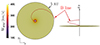 |
Fig. 1. Inner region of the MHD simulation. Top and side view of the heliographic equatorial plane, colored with the velocity of the solar wind usw after steady state has been reached. An anti-sunward magnetic field line emanating from the domain at 24° latitude is also shown in red. |
2.2. Particle dynamics: Guiding center approximation
In the GCA, the relativistic motion of a test particle of rest mass m and electric charge q is described by the following set of equations (see, e.g., Ripperda et al. 2017):
![$$ \begin{aligned} \frac{\mathrm{d}\boldsymbol{R}}{\mathrm{d}t}&= v_{\Vert }\boldsymbol{b} + \boldsymbol{v}_{E} + \frac{\gamma m}{qB}\boldsymbol{b} \nonumber \\&\times \left[ \frac{\mu _{B}}{\gamma ^2 m} \nabla B + \frac{v_{\Vert }}{\gamma }E_{\Vert }\boldsymbol{v}_{E} + v_{\Vert }^2\left(\boldsymbol{b}\cdot \nabla \right)\boldsymbol{b} \right. \nonumber \\&+\left. v_{\Vert }( \left(\boldsymbol{v}_{E}\cdot \nabla \right)\boldsymbol{b} + \left(\boldsymbol{b}\cdot \nabla \right)\boldsymbol{v}_{E}) + \left(\boldsymbol{v}_{E}\cdot \nabla \right)\boldsymbol{v}_{E} \right] \end{aligned} $$](/articles/aa/full_html/2025/02/aa51436-24/aa51436-24-eq4.gif)
![$$ \begin{aligned} \frac{\mathrm{d} (\gamma v_{\Vert })}{\mathrm{d}t}&= \frac{q}{m}E_{\Vert } - \frac{\mu _{B}}{\gamma m}\boldsymbol{b}\cdot \nabla B \nonumber \\&+ \gamma \boldsymbol{v}_{E}\cdot \left[ v_{\Vert }\left(\boldsymbol{b}\cdot \nabla \right)\boldsymbol{b}+ \left(\boldsymbol{v}_{E}\cdot \nabla \right)\boldsymbol{b} \right] \end{aligned} $$](/articles/aa/full_html/2025/02/aa51436-24/aa51436-24-eq5.gif)

In the above equations, the subscripts ∥ and ⊥ indicate projections parallel and perpendicular with respect to B. R is the position of the particle guiding center, and v the guiding center velocity,  is its Lorentz factor (with c the speed of light). Hence, hereafter, ℰ = (γ − 1)mc2 denotes the relativistic kinetic energy of the particle.
  is its magnetic moment, and vE ≡ E × b/B is the E-cross-B drift velocity, where b ≡ B/B is the unit vector along B. In ideal MHD, the electric field is given by E = −u × B (ideal Ohm’s law), where u is the velocity of the fluid. However, since the electric field enters the system of MHD equations through ∂B/∂t = −∇×E, an irrotational component can be added to the electric field without affecting the MHD flow. The contribution of the charge neutralizing electrostatic field due to the electron fluid −∇pe/(ene) can be considered and the nonideal two-fluid Ohm law E = −u × B − ∇pe/(ene) can be used, where e is the positive elementary charge, pe is the electron pressure, and ne is the electron number density. We assumed a fully ionized electron–proton plasma so that we can write ∇pe/ne = 2κ(1 + κ)−1∇p/n, where κ ≡ Te/Tp is the electron-to-proton temperature ratio, which we set to κ = 1. The expression for the electric field used in the particles simulations is therefore
The corrected field is not irrotational in general. However, since p = p0 and n = n0 over the whole inner boundary, since all fluid particles in the domain emanate from the inner boundary, and since p/nΓ is constant along streamlines (Γ is the adiabatic index), it follows that p = p(n) and therefore ∇ × (∇p/n) = 0, as required. The wind simulation was compatible with the two-fluid Ohm law, and we therefore used it to evaluate the electric field in the simulated wind. We note, however, that the large-scale electrostatic field is generally of minor importance for SEP particles as the difference of electrostatic potential between the corona and r = 1 AU is only about a few hundred Volt, which becomes relevant for SEP particles below a few keV. We note that the above GCA equations are for nonrelativistic flows with |u|≪c, a condition that is largely satisfied in the solar wind (relativistic flows were considered in Ripperda et al. (2017)).
The positions and velocity of test particles were advanced in time according to the GCA Equations (1)–(3) and the fields from the MHD simulation. We used a trilinear interpolation from the MHD grid to evaluate the fields at the particle position. Particles were advanced in time using the third-order prediction-correction time-integration scheme by Mignone et al. (2023), which we briefly outline below.
We set X ≡ {R, γv∥} and denote F to be the right-hand-side terms of the Equations (1)–(2). We then write the GCA equations as

Integration of Eq. (4) from a time level tn to tn + 1 = tn + Δtn was made by a predictor step followed by a corrector step,
![$$ \begin{aligned} \boldsymbol{X}^*&= \boldsymbol{X}^n \nonumber \\&+ \Delta t^n \left[ \left( 1 + \frac{\tau ^n}{2} \right) \boldsymbol{F}^n- \frac{\tau ^n}{2} \boldsymbol{F}^{n-1} \right] + \mathcal{O} (\Delta t^3) \end{aligned} $$](/articles/aa/full_html/2025/02/aa51436-24/aa51436-24-eq11.gif)
![$$ \begin{aligned} \boldsymbol{X}^{n+1}&= \boldsymbol{X}^n \nonumber \\&+ \frac{\Delta t^n}{6(1+\tau ^n)} \left[ 3 \left(\boldsymbol{F}^n + \boldsymbol{F}^{*}\right) + 4 \tau ^n \left(\boldsymbol{F}^{n}+\frac{\boldsymbol{F}^{*}}{2}\right) \right. \nonumber \\&+ (\tau ^n)^2 (\boldsymbol{F}^{n} - \boldsymbol{F}^{n-1}) \left. \right] + \mathcal{O} (\Delta t^4), \end{aligned} $$](/articles/aa/full_html/2025/02/aa51436-24/aa51436-24-eq12.gif)
where Xn = X(tn), Fn = F(Xn) and τn ≡ Δtn/Δtn − 1. We highlight that the factor 3 in Eq. (6) is missing in the corresponding Equation (15) of Mignone et al. (2023). At t = 0, or after a collision, the unknown quantities at tn − 1 were computed with a simple backward Euler step: Xn − 1 = Xn − ΔtnFn.
2.3. Pitch-angle scattering
In the solar wind, the mean free path for Coulomb collisions is about 1 AU for thermal ions and electrons. Since it grows as v4, Coulomb collisions are completely ineffective for energetic particles. However, energetic particles are diffused in velocity space by turbulent fluctuations of the electromagnetic field of the wind (Parker 1965). A quasi-linear theory of the pitch-angle diffusion of charged particles in a weak turbulent magnetic field superposed on a strong guiding field, based on the Fokker-Planck equation, was first developed by Jokipii (1966, 1968). For power-law turbulence and nearly isotropic distributions, the quasi-linear phase-space diffusion coefficient takes the general form
where μ ≡ cos α, and α is the angle between the particle velocity v and the magnetic field B, and h(μ) is a model-dependent function (see Schlickeiser (1989), Wijsen et al. (2019)). A parallel mean free path λ∥ can be computed from the diffusion coefficient (Jokipii 1966; Hasselmann & Wibberenz 1968; Bieber et al. 1994) via
For constant h(μ) = h0 in Eq. (7), h0 = v/λ∥, which can thus be interpreted as the collision frequency for μ = 1 (or α = 0°) particles. In Equation (8) the parallel mean free path depends on the velocity. However, since Dμμ(μ) is proportional to the collision frequency, v/⟨Dμμ⟩ can be interpreted as a measure of the distance between scattering centers, and λ∥ is expected to be only weakly dependent on the particle energy. At 1 AU, the observed mean free paths of protons and electrons are in the range 0.1–1 AU for a large interval of rigidities from 10−4 MV to 104 MV (Palmer 1982; Bieber et al. 1994).
Diffusion is generally thought to occur through the accumulation of small deviations. This can be simulated numerically by applying a Fokker-Planck diffusion operator to an initial distribution of particles. We adopted a different approach in which test particles underwent hard-sphere-type collisions as in Marsh et al. (2013) and Dalla et al. (2013, 2015). In practice, for a particle that covered a distance Δs = ∫0Δtv∥dt during the time step Δt, the collision probability is given by

At each time step, a random number a is generated in the interval [0, 1]. If a < p(Δs), the particle undergoes an elastic collision. In the case of a collision, the post-collision pitch angle α = arccos(μ) (in the frame of the scattering centers) is selected to give a uniform distribution in μ
![$$ \begin{aligned} \mu = 1-2a,\; {a:\,\mathrm{random number}}\in [0,1]. \end{aligned} $$](/articles/aa/full_html/2025/02/aa51436-24/aa51436-24-eq16.gif)
Given the scattering law (10), all directions in 3D space are equally probable. The law does not ensure isotropy, however. The reason is that since the particle guiding centers move along the magnetic field at an angle-dependent speed μv, the scattering centers do not receive an isotropic distribution while emitting an isotropic distribution under the action of the scattering law (10). As a result, collisions tend to overpopulate the directions perpendicular to the magnetic field. To force isotropy in the highly collisional limit, the post-collision angular distribution of the particles hitting the scattering centers must be equal to the pre-collision distribution. The latter is obviously proportional to the rate at which particles from an isotropic distribution hit the scattering centers during their one-dimensional displacement along the magnetic field. The number n of scattering events per time unit observed at a scattering center with a pitch angle α such that cos α > |μ| is given by (see Sect. II.C in Pantellini 2000)
where n0 is the cumulated number of events for μ in the range [ − 1, 1]. In this case, n varies linearly with respect to μ2 instead of μ, and the scattering law (10) has to be modified accordingly,
![$$ \begin{aligned} \mu = \pm \sqrt{a},\; {a:\,\mathrm{random number}}\in [0,1] , \end{aligned} $$](/articles/aa/full_html/2025/02/aa51436-24/aa51436-24-eq18.gif)
with the plus and minus sign being equally probable. The mean free path λ∥ is the distance between the scattering centers and is therefore identical for all particles, that is, λ∥ = v∥/ν(μ) = v/ν0, where ν(μ) = ν0μ is the particle collision frequency. From Eq. (8) and the general form of Dμμ Eq. (7), it follows that the corresponding Fokker-Planck diffusion coefficient is Dμμ = ν0(1 − μ2)/2, which is the form used by Zaslavsky et al. (2024). Hence, differences between our results and those of Zaslavsky et al. (2024) are expected for a scattering model other than Eq. (12). Since there are no stringent reasons for the distribution of test particles to be isotropized by the scattering, we adopt the scattering law (10) for which all post-scattering directions are equally probable in the following, but we retain that the diffusion in phase-space is not of the Fokker-Planck type.
3. Results and discussion
Initially, 103 mono-energetic electrons were impulsively injected with 81 keV energy and α = 0 at r = 0.28 AU (corresponding to 60 R⊙) and 24° latitude on the corotating magnetic field line shown in Fig. 1. The choice of α = 0 was arbitrary and did not significantly impact the results because the mirror force naturally drives the perpendicular velocity toward zero as particles propagate outward in the decreasing magnetic field. We set λ∥ to three different values {0.1, 0.5, and 1} AU in three different simulations, in conformity with the consensus on the mean free path of high-energy particles near 1 AU (Palmer 1982; Bieber et al. 1994). In the following, except in Sect. 3.3, we focus exclusively on the case of λ∥ = 0.5 AU. We adopted a constant time step Δt = 0.54 s to integrate the GCA equations and perform scattering in the inertial frame so that the particles did not experience adiabatic cooling (cf. Sect. 3.2). Particles that left the spherical shell [0.28, 5] AU1 were reinitialized (reborn) on the same magnetic line with the same initial velocity during 150 h, which was long enough for each particle to be reborn 20 times on average. To check for a steady state, we monitored the time evolution of the mean heliocentric distance of the particles. When this quantity stabilized, we considered the system to have reached steady state. This occurred around t = 8.3 h. We were primarily interested in the steady-state distribution of particles, so that in the following, we only consider particles that were injected after t = 8.3 h. To make statistics, we accumulated snapshots of the system every 100 time steps (=54 s, roughly one-tenth of the collision time), which is equivalent to an ensemble of some 9.4 106 electrons. As an example, a snapshot of the spatial distribution and the energy of the electrons at t ∼ 30 h is reported in Fig. 2. The figure shows that particles are dominated by a vE drift in the azimuthal direction (toward positive φ). Even if this drift, which scales with the solar wind velocity (∼400 km/s), is much faster than both the curvature and gradient drifts (see below), it does not contribute to the particle energy loss from 81 to 76 keV. The reason is that the vE drift is by definition transverse to the electric field and only displaces particles on equipotential lines. Particles may change their energy when they move along the magnetic field line (first term on the right-hand side of Eq. (1) because of the nonzero field-aligned electrostatic field E∥, but as already mentioned, this field is weak, especially at heliocentric distances beyond the sonic point. We considered the two dominant drifts (for particles with v ≫ usw) from the square brackets on the right-hand side of Eq. (1). These are the curvature drift velocity
![$$ \begin{aligned} \boldsymbol{v}_{\rm curv} = [\gamma m v_{\Vert }^2 /(q B)]\,\boldsymbol{b} \times (\boldsymbol{b}\cdot \nabla ) \boldsymbol{b}, \end{aligned} $$](/articles/aa/full_html/2025/02/aa51436-24/aa51436-24-eq19.gif)
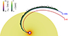 |
Fig. 2. Top view of the spatial distribution of the electrons at t = 30 h. In blue we plot the field line on which the particles were injected. In red we plot the same field line t = 30 h earlier, at the time of the injection of the oldest particles. |
and the gradient drift velocity
![$$ \begin{aligned} \boldsymbol{v}_{\nabla B} = [\gamma m v_{\perp }^2 /(2 q B)]\,\boldsymbol{b} \times \nabla \mathrm{ln} B. \end{aligned} $$](/articles/aa/full_html/2025/02/aa51436-24/aa51436-24-eq20.gif)
We anticipate that for a ℰ = 81 keV electron (or proton) in a B = 1 nT field and typical magnetic gradient scales of about LB = 1 AU, the expected drift velocities are low as vcurv ∼ v∇B ∼ ℰ/(eBLB)≈0.5 km/s. For a fixed kinetic energy (i.e., for a fixed v), both terms can be written in terms of sin2α as v⊥2 = v2sin2α and v∥2 = v2(1 − sin2α). Averages of sin2α as a function of heliocentric distance are reported in Fig. 3 for the λ∥ = 0.5 AU simulation. The figure shows that the pitch-angle distribution tends to evolve from beam-like to isotropic with increasing distance, indicating a decreasing efficiency of the magnetic focusing. The variations in the curvature and gradient drift with heliocentric distance clearly depend on the variation in α and both the variation in the magnetic curvature and the magnetic gradient in the plane perpendicular to B. The radial profiles of all components of vcurv(r) and v∇B(r) are plotted in Fig. 4 for a constant sin2α = 0.64 (average value from the curve in Fig. 3). The drifts are charge dependent (protons and electrons drift in opposite directions), and their main components along θ increase linearly for r ≲ 1.5 AU and become nearly constant for r ≳ 2 AU. In this configuration, both drifts correspond to a poleward motion of the electrons (toward decreasing θ) and an equatorward motion of the protons. Both drifts are slow but perpendicular to the fast vE drift. In Fig. 2, black particles have experienced greater drift in longitude and latitude, and their energy loss is consequently greater.
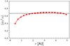 |
Fig. 3. Simulation with λ∥ = 0.5 AU. Pitch-angle distribution ⟨sin2α⟩ as a function of heliocentric distance. The dashed horizontal line corresponds to the isotropic distribution for which ⟨sin2α⟩ = 2/3. |
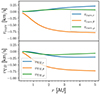 |
Fig. 4. Simulation with λ∥ = 0.5 AU. Radial variations in the components of the curvature drift (top panel) and magnetic gradient drift (bottom panel) for a 81 keV electron with a constant pitch sin2α = 0.64. |
3.1. Energy loss
From an order-of-magnitude estimate of the terms in Eq. (2), it is clear that for 81 keV electrons, energy changes are essentially caused by the field curvature and field gradient terms. Assuming time steadiness, we write Eq. (2) in terms of the time evolution of the kinetic energy of a particle,
In this configuration, vE is oriented opposite to the curvature vector (b⋅∇)b and to the magnetic field gradient ∇lnB, so that Eq. (13) describes a systematic loss of energy, regardless of whether the particle is moving away from or toward the Sun (also see Fig. 2 in Dalla et al. 2015).
Replacing vE with E × b/B, we write Eq. (13) as

where vd = vcurv + v∇B is the total drift velocity. Equation (14) shows that energy loss is due to the electrons that drift along the electric field, whose main component is in the −θ direction. Protons also lose energy, as they drift in the opposite direction. It is evident that particles lose energy independently of their charge because the charge does not appear in Eq. (13) (see also Dalla et al. 2015).
The loss rate computed from the right-hand side of Eq. (13) is reported in the bottom panel of Fig. 5 for the two values of sin2α that correspond to the extreme cases in Fig. 3. For the wind conditions in our simulation, the maximum loss rate occurs at r = 1.2 AU. Toward increasing r, the loss rate drops because the curvature and magnetic gradient scale of the magnetic field lines increase. Toward decreasing r, the loss rate drops because of the decreasing vE, as the fluid velocity and the magnetic field tend to align when they approach the inner boundary.
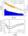 |
Fig. 5. Simulation with λ∥ = 0.5 AU. Top: energy vs. age (time since injection) for electrons near r = 1 AU. Linear fits of the decay rate for young (age < 4 h) and old (age ≥ 4 h) electrons are given. The normalized age distribution is also plotted. Bottom: Average energy-loss rate as a function of heliocentric distance r given by Eq. (13) for the extreme values of sin2α observed in Fig. 3. |
The loss of kinetic energy as a function of age (time since injection) for particles in the range r ∈ [0.9, 1.1] AU is shown in the top panel of Fig. 5. The difference between young (age < 4 h) and old (age ≥ 4 h) can be understood in the line of the energy loss rate in the bottom panel of Fig. 5. Young particles did not have the opportunity to spend long periods of time at large heliocentric distances where the energy loss rate is substantially lower than near 1.2 AU, so that they lost energy faster than the old particles on average. As the energy loss rate is proportional to v∥2 and because collisions tend to isotropize the pitch-angle distribution, the energy loss rate might be thought to depend on the mean free path λ∥. Figure 6 shows that the differences are relatively small for the λ∥ values {0.1, 0.5, and 1} AU. As we showed in the bottom panel of Fig. 5, the energy loss rate depends on the pitch-angle distribution. The smaller ⟨sin2α⟩, the higher the energy loss rate, as for this wind configuration near 1 AU the curvature term is a more efficient cooler than the magnetic gradient term in Eq. (13). This explains the fast energy loss for young particles that spent most of their lifetime near 1 AU, where sin2α is comparatively small. As particles grow older, the loss rate is reduced because old particles spent a significant fraction of their lives at large heliocentric distances, where sin2α is largest. The average displacement of a particle with respect to the observation point can be evaluated by assuming that the motion of the particle is a random walk. Its displacement with respect to the observation point at r = 1 AU might then be estimated to be about  , where N ∼ vt/λ∥ is the number of collisions during the time t. For particles aged ta = 9h (ta is the time since injection) moving at v = c/2, the displacement
  is about {1.8; 4.0; 5.7} AU for λ∥ = {0.1; 0.5; 1} AU, respectively. Hence, as loss rates decrease at more than 1 AU from the observation point (see the bottom panel of Fig. 5), loss rates are logically lower for old particles and a long collisional mean free path λ∥. For comparison, the displacement is three times weaker and the age effect is negligible for particles that are only 1h old.
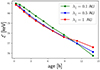 |
Fig. 6. Energy profiles as a function of age for electrons near r = 1 AU and different values of λ∥. |
3.2. Adiabatic cooling
To distinguish the energy losses caused by the drifts from the energy losses caused by the scattering, we so far considered the case in which the scattering centers do not move with respect to the fixed inertial frame attached to the Sun. In this frame, the particle energy is conserved during collisions. However, when we assume that the scattering is due to the turbulence in the solar wind plasma, the appropriate frame for the scattering is the solar wind frame. Because of the combined action of scattering and magnetic focusing, the magnitude of the particle momentum  in this case changes in time according to (see e.g. Ruffolo 1995)
where the tilde quantities refer to the moving frame. In a radial field B ∝ 1/r2 and in the limit of frequent scattering (i.e., λ∥ ≪ |LB|), the average particle position moves radially outward at a speed usw, so that it sees a decreasing magnetic field and an average ⟨LB⟩=r/2. In the extreme case of frequent scattering, the pitch-angle distribution is close to isotropic, in which case  and Eq. (15) reduces to
Equation (16) predicts a loss rate of −1.34% per hour, which in terms of kinetic energy loss rate corresponds to a loss rate of about −1 keV/h for a 81 keV electron. This is an upper estimate of the cooling rate, as for infrequent collisions, particles tend to accumulate near  , which reduces the loss rate to zero.
The energy loss that arises from the movement of the scattering center with the solar wind is shown in Fig. 7. The only other difference with respect to the simulation of Fig. 5 is that solely the drift parallel to B is retained in the GCA equations. The large dispersion in energy clearly arises because all pitch angles α in the range 0–180° are accessible, with each value of α giving a different cooling rate, as expressed by Eq. (15). Figure 7 shows that the adiabatic loss rate continuously decreases with age, for instance, from −1.8 keV/h for particles aged 0.3 h to −0.6 keV/h for particles aged 1 h and −0.3 keV/h for particles aged 4 h. The reason is that the average heliocentric position ⟨r⟩ of very young particles is about the r0 (observer’s position) and  for old particles aged ≫r02/(vswλ∥). Setting r = ⟨r⟩ in Eq. (16), we obtain a loss rate ∼vsw/r0 for young particles and an age-dependent loss rate
  for old particles.
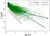 |
Fig. 7. Energy vs. age near r = 1 AU for electrons undergoing scattering in the solar wind frame with all drifts, except for v∥b, turned off. As in Fig. 5, the initial energy of the electrons is 81 keV, and the scattering mean free path is λ∥ = 0.5 AU. The black line shows the average evolution. The slopes corresponding to the theoretical loss rates from the expression (16) for a radial magnetic field and a wind velocity usw = 418 km/s are also shown. |
Figure 8 illustrates the contribution of the adiabatic cooling to the global energy loss rate for the case λ∥ = 0.5 AU. The orange dots are from Fig. 5 without adiabatic cooling particles (scattering in the fixed frame). The green dots correspond to the same simulation, except that the scattering centers are in the wind frame instead of the fixed frame. As already suggested by Fig. 7, the adiabatic cooling is the dominant cooling mechanism for young particles. For particles aged 0.3 h, it contributes −1.8 keV/h to the total loss rate of −2.1 keV/h. For particles older than −1.5 h, the contribution of the adiabatic cooling is small, which is confirmed by the fact that the energy versus age profile for the green dots is only marginally steeper than for the orange dots. As an example, at age 9 h, the cooling rates are about −0.4 keV/h and −0.3 keV/h, respectively.
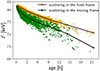 |
Fig. 8. Simulations with λ∥ = 0.5 AU. The energy as a function of age near r = 1 AU is shown considering only drift effects (orange dots) and considering both drifts and adiabatic cooling effects (green dots). The average profiles are also plotted for both cases. |
3.3. Pitch-angle distribution
In the case of a transient injection, for example, due to a solar particle event, the flux of 81 keV electrons at 1 AU reaches its peak ∼10 min after injection. As the peak intensity rapidly decreases on a timescale of about 10–20 minutes, only electrons younger than 20 min are representative of electrons from a solar particle event at the time of strongest particle flux at 1 AU. Retaining particles aged 20 minutes or less is equivalent to measuring the flux of particles from a solar event at 1 AU over a 10-minute interval.
The pitch-angle distribution of these young electrons is plotted in Fig. 9 and is compared with measurements from the Wind spacecraft during a 9-minute interval following the peak of the 20 October 2002 solar event. In order to temper the dependence on the initial condition (in our case, v⊥ = 0 and therefore μB = 0), only electrons that experienced at least one collision were retained in Fig. 9. This is the reason for the deficit of particles for α → 180°. Other parts of the distribution are likely slightly affected by choice of the initial condition, as the mean free path λ∥ = 0.5 AU is not much shorter than the distance between the injection point and the observation point at 1 AU. It is interesting to note that the differences with respect to the measurements of Dröge et al. (2018) are minor, despite the relative arbitrariness of the wind model, initial conditions, mean free path, and injection point adopted in the model. The angular distribution of young electrons is more strongly field aligned than the steady-state distribution, as expected, including electrons of all ages (see the inset in Fig. 9 for λ∥ = 0.5 AU). The latter is also shown in the middle panel of Fig. 10, where it is compared to the distribution Kexp(Kcos α)/(2sinh(K)) obtained by Zaslavsky et al. (2024) from a Fokker-Planck-type equation in the limit of a spatially constant Knudsen number K = λ∥/LB. The top and bottom panels of Fig. 10 display the results for the cases λ∥ = 0.1 AU and λ∥ = 1 AU, respectively. We note that as λ∥ decreases, the distribution becomes isotropic in the Fokker-Planck model, but not in our particle model. As already discussed thoroughly at the end of Sect. 3.3, this is a property of the scattering law (10) when it is applied to particles that aer constrained to move in one dimension.
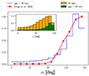 |
Fig. 9. Normalized pitch-angle distribution for 81 keV electrons younger than 20 min with λ∥ = 0.5 AU compared to electron measurements in the range 49–81 keV from the Wind 3DP SST instrument for the 20 October 2002 14:30 solar energetic particle event (adapted from Dröge et al. 2018). |
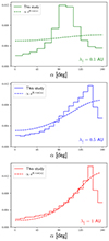 |
Fig. 10. Normalized steady-state (i.e., all ages) pitch-angle distribution for 81 keV electrons with λ∥ = 0.1 AU (top), λ∥ = 0.5 AU (middle), and λ∥ = 1 AU (bottom). The constant Knudsen predictions from a simple Fokker-Planck model are plotted as well (Zaslavsky et al. 2024), with the Knudsen numbers K = 0.11 (top), K = 0.54 (middle), and K = 1.08 (bottom) computed from the model values at 1 AU (see Table 1). |
4. Conclusion
The trajectories and the distribution of energetic test electrons propagating in the field of a simulated solar wind were obtained by integrating the relativistic GCA equations of motion using the 𝒪(Δt3) predictor-corrector scheme that was first proposed by Mignone et al. (2023). In order to mimic their interaction with small-scale plasma turbulence, which is not included in the solar wind simulation, particles were also scattered by hard-sphere type collisions. Following the consensus on the scattering mean free path of high-energy particles in the solar wind (Palmer 1982; Bieber et al. 1994), we adopted a mean free path λ∥ of the order of the astronomical unit.
In our case study, we computed the evolution of 81 keV test electrons continuously injected at r = 0.28 AU and 24° latitude on a corotating magnetic field line in a MHD simulation of a standard steady solar wind. For a parallel mean free path λ∥ = 0.5 AU, the flux of particles observed near 1 AU is roughly an exponential function of age, the flux of particles aged 30 h is lower by some 104 than the flux of particles aged 1h (see the top of Fig. 5). The main outcomes are summarized below.
-
The pitch-angle distribution of young electrons (younger than 20 min and representative of the electrons observed minutes after a solar particle event) compares well with the distribution of electrons in the energy range 49–81 keV observed by the WIND spacecraft after the 20 October 2002 14:30 SEP events. This confirms that λ∥ = 0.5 AU is a good estimate of the mean free path of 𝒪(102 keV) electrons near 1 AU (see, e.g., Palmer (1982), Bieber et al. (1994)).
-
Electrons systematically lose energy due to their slow poleward motion against the advection electric field because of the curvature drift and the gradient drift.
-
For electrons younger than 4 h, the drift-induced loss rate is a relatively fast rate of 0.7 keV/h.
-
For electrons older than 4 h, the drift-induced loss rate is lower by a factor 2.
-
Adiabatic cooling is dominant for particles younger than 1.5 h, for which it is about 1.8 keV/h given a total (drift + adiabatic) loss rate of 2.1 keV/h.
-
For particles aged 1.5 h, drift and adiabatic loss rates are comparable. For particles older than 1.5 h, the adiabatic loss rate is of secondary importance as its contribution decreases with age roughly as
 .
.
Our test-particle propagation method differs from the method introduced by Marsh et al. (2013) that was subsequently used by Dalla et al. (2013, 2015). In these works, particles were advanced in the electromagnetic field of an analytic wind model by integrating the general form of the equation of motion. Instead, we propagated particles in the electromagnetic field of a simulated solar wind, with the possibility to include dynamical effects such as CMEs. Instead of integrating the full equations of motion, we also integrated the equations in the guiding-center approximation, which allowed us to remove the extremely restrictive requirement of having to use a time step much shorter than the gyration period. This allowed us to use time steps that were longer by several orders and resulted in substantially faster simulations and smaller accumulated numerical errors.
This work is a first step of a work in progress. Taking advantage of the unprecedentedly large number of spacecraft that currently travel through the inner heliosphere, our next step is to apply our method to the case of relativistic electrons or protons in the field of a nonstationary solar wind that is traversed by one or several CMEs.
Acknowledgments
The authors wish to thank Arnaud Zaslavsky for fruitful discussions. Ahmed Houeibib is supported by the CNES (Centre National d’Études Spatiales). This work has been financially supported by the PLAS@PAR project and by the National Institute of Sciences of the Universe (INSU).
References
- Bieber, J. W., Matthaeus, W. H., Smith, C. W., et al. 1994, ApJ, 420, 294 [Google Scholar]
- Chhiber, R., Subedi, P., Usmanov, A. V., et al. 2017, The Astrophysical Journal Supplement Series, 230, 21 [NASA ADS] [CrossRef] [Google Scholar]
- Cliver, E. W. 2009, in Universal Heliophysical Processes, eds. N. Gopalswamy, & D. F. Webb, IAU Symposium, 257, 401 [NASA ADS] [Google Scholar]
- Dalla, S., Marsh, M. S., Kelly, J., & Laitinen, T. 2013, Journal of Geophysical Research (Space Physics), 118, 5979 [NASA ADS] [CrossRef] [Google Scholar]
- Dalla, S., Marsh, M. S., & Laitinen, T. 2015, ApJ, 808, 62 [NASA ADS] [CrossRef] [Google Scholar]
- Desai, M., & Giacalone, J. 2016, Living Reviews in Solar Physics, 13, 3 [NASA ADS] [CrossRef] [Google Scholar]
- Dröge, W., Kartavykh, Y. Y., Wang, L., Telloni, D., & Bruno, R. 2018, The Astrophysical Journal, 869, 168 [CrossRef] [Google Scholar]
- Forbush, S. E. 1946, Phys. Rev., 70, 771 [Google Scholar]
- Ginzburg, V. L., & Zhelezniakov, V. V. 1958, Sov. Astron., 2, 653 [Google Scholar]
- Griton, L., Pantellini, F., & Meliani, Z. 2018, Journal of Geophysical Research (Space Physics), 123, 5394 [NASA ADS] [CrossRef] [Google Scholar]
- Hasselmann, K., & Wibberenz, G. 1968, Zeitschrift für Geophysik, 34, 353 [Google Scholar]
- Jokipii, J. R. 1966, ApJ, 146, 480 [Google Scholar]
- Jokipii, J. R. 1968, ApJ, 152, 671 [NASA ADS] [CrossRef] [Google Scholar]
- Klein, K.-L., & Dalla, S. 2017, Space Science Reviews, 212, 1107 [NASA ADS] [CrossRef] [Google Scholar]
- Marsh, M. S., Dalla, S., Kelly, J., & Laitinen, T. 2013, The Astrophysical Journal, 774, 4 [NASA ADS] [CrossRef] [Google Scholar]
- Mignone, A., Haudemand, H., & Puzzoni, E. 2023, Computer Physics Communications, 285, 108625 [NASA ADS] [CrossRef] [Google Scholar]
- Palmer, I. D. 1982, Reviews of Geophysics and Space Physics, 20, 335 [NASA ADS] [CrossRef] [Google Scholar]
- Pantellini, F. G. E. 2000, American Journal of Physics, 68, 61 [NASA ADS] [CrossRef] [Google Scholar]
- Parker, E. 1965, Planetary and Space Science, 13, 9 [NASA ADS] [CrossRef] [Google Scholar]
- Payne-Scott, R., Yabsley, D. E., & Bolton, J. G. 1947, Nature, 160, 256 [NASA ADS] [CrossRef] [Google Scholar]
- Reames, D. V. 1999, Space Science Reviews, 90, 413 [NASA ADS] [CrossRef] [Google Scholar]
- Ripperda, B., Porth, O., Xia, C., & Keppens, R. 2017, MNRAS, 467, 3279 [NASA ADS] [Google Scholar]
- Ruffolo, D. 1995, ApJ, 442, 861 [Google Scholar]
- Schlickeiser, R. 1989, ApJ, 336, 243 [NASA ADS] [CrossRef] [Google Scholar]
- Tanaka, T. 1994, Journal of Computational Physics, 111, 381 [CrossRef] [Google Scholar]
- Wijsen, N., Aran, A., Pomoell, J., & Poedts, S. 2019, A&A, 622, A28 [NASA ADS] [CrossRef] [EDP Sciences] [Google Scholar]
- Wijsen, N., Aran, A., Sanahuja, B., Pomoell, J., & Poedts, S. 2020, A&A, 634, A82 [NASA ADS] [CrossRef] [EDP Sciences] [Google Scholar]
- Wijsen, N., Aran, A., Scolini, C., et al. 2022, A&A, 659, A187 [NASA ADS] [CrossRef] [EDP Sciences] [Google Scholar]
- Wild, J. P., & McCready, L. L. 1950, Australian Journal of Chemistry, 3, 387 [CrossRef] [Google Scholar]
- Wild, J. P., Smerd, S. F., & Weiss, A. A. 1963, Annual Review of Astronomy and Astrophysics, 1, 291 [NASA ADS] [CrossRef] [Google Scholar]
- Xia, C., Teunissen, J., El Mellah, I., Chané, E., & Keppens, R. 2018, ApJS, 234, 30 [Google Scholar]
- Zaslavsky, A., Kasper, J. C., Kontar, E. P., et al. 2024, The Astrophysical Journal, 966, 60 [NASA ADS] [CrossRef] [Google Scholar]
All Tables
All Figures
|
Fig. 1. Inner region of the MHD simulation. Top and side view of the heliographic equatorial plane, colored with the velocity of the solar wind usw after steady state has been reached. An anti-sunward magnetic field line emanating from the domain at 24° latitude is also shown in red. |
| In the text | |
|
Fig. 2. Top view of the spatial distribution of the electrons at t = 30 h. In blue we plot the field line on which the particles were injected. In red we plot the same field line t = 30 h earlier, at the time of the injection of the oldest particles. |
| In the text | |
|
Fig. 3. Simulation with λ∥ = 0.5 AU. Pitch-angle distribution ⟨sin2α⟩ as a function of heliocentric distance. The dashed horizontal line corresponds to the isotropic distribution for which ⟨sin2α⟩ = 2/3. |
| In the text | |
|
Fig. 4. Simulation with λ∥ = 0.5 AU. Radial variations in the components of the curvature drift (top panel) and magnetic gradient drift (bottom panel) for a 81 keV electron with a constant pitch sin2α = 0.64. |
| In the text | |
|
Fig. 5. Simulation with λ∥ = 0.5 AU. Top: energy vs. age (time since injection) for electrons near r = 1 AU. Linear fits of the decay rate for young (age < 4 h) and old (age ≥ 4 h) electrons are given. The normalized age distribution is also plotted. Bottom: Average energy-loss rate as a function of heliocentric distance r given by Eq. (13) for the extreme values of sin2α observed in Fig. 3. |
| In the text | |
|
Fig. 6. Energy profiles as a function of age for electrons near r = 1 AU and different values of λ∥. |
| In the text | |
|
Fig. 7. Energy vs. age near r = 1 AU for electrons undergoing scattering in the solar wind frame with all drifts, except for v∥b, turned off. As in Fig. 5, the initial energy of the electrons is 81 keV, and the scattering mean free path is λ∥ = 0.5 AU. The black line shows the average evolution. The slopes corresponding to the theoretical loss rates from the expression (16) for a radial magnetic field and a wind velocity usw = 418 km/s are also shown. |
| In the text | |
|
Fig. 8. Simulations with λ∥ = 0.5 AU. The energy as a function of age near r = 1 AU is shown considering only drift effects (orange dots) and considering both drifts and adiabatic cooling effects (green dots). The average profiles are also plotted for both cases. |
| In the text | |
|
Fig. 9. Normalized pitch-angle distribution for 81 keV electrons younger than 20 min with λ∥ = 0.5 AU compared to electron measurements in the range 49–81 keV from the Wind 3DP SST instrument for the 20 October 2002 14:30 solar energetic particle event (adapted from Dröge et al. 2018). |
| In the text | |
|
Fig. 10. Normalized steady-state (i.e., all ages) pitch-angle distribution for 81 keV electrons with λ∥ = 0.1 AU (top), λ∥ = 0.5 AU (middle), and λ∥ = 1 AU (bottom). The constant Knudsen predictions from a simple Fokker-Planck model are plotted as well (Zaslavsky et al. 2024), with the Knudsen numbers K = 0.11 (top), K = 0.54 (middle), and K = 1.08 (bottom) computed from the model values at 1 AU (see Table 1). |
| In the text | |
Current usage metrics show cumulative count of Article Views (full-text article views including HTML views, PDF and ePub downloads, according to the available data) and Abstracts Views on Vision4Press platform.
Data correspond to usage on the plateform after 2015. The current usage metrics is available 48-96 hours after online publication and is updated daily on week days.
Initial download of the metrics may take a while.