| Issue |
A&A
Volume 682, February 2024
|
|
|---|---|---|
| Article Number | A82 | |
| Number of page(s) | 14 | |
| Section | The Sun and the Heliosphere | |
| DOI | https://doi.org/10.1051/0004-6361/202347248 | |
| Published online | 02 February 2024 | |
Modeling energetic proton transport in a corotating interaction region
An energetic particle event observed by STEREO-A from 21 to 24 August 2016
1
State Key Laboratory of Space Weather, National Space Scinece Center, Chinese Academy of Sicences, Beijing, PR China
e-mail: fshen@spaceweather.ac.cn
2
Shangdong Institute of Advanced Technology, Jinan, PR China
3
College of Earth and Planetary Sciences, University of Chinese Academy of Scineces, Beijing, PR China
4
Key Laboratory of Solar Activity and Space Weather, National Space Scinece Center, Chinese Academy of Sicences, Beijing, PR China
5
Key Laboratory of Space Weather, National Satellite Meteorological Center (National Center for Space Weather), China Meteorological Adminstration, Bejing, PR China
Received:
21
June
2023
Accepted:
14
November
2023
Aims. An energetic particle event related to a corotating interaction region (CIR) structure was observed by the Solar-Terrestrial Relations Observatory-A (STEREO-A) from 21 to 24 August 2016. Based on an analysis of measurement data, we suggest that instead of being accelerated by distant shocks, a local mechanism similar to diffusive shock acceleration (DSA) acting in the compression region could explain the flux enhancements of 1.8–10.0 MeV nucleon−1 protons. We created simulations to verify our hypothesis.
Methods. We developed a coupled model composed of a data-driven analytical background model providing solar wind configuration and a particle transport model represented by the focused transport equation (FTE). We simulated particle transport in the CIR region of interest in order to obtain the evolution of proton fluxes and derive the spectra.
Results. We find that the simulation is well correlated with the observation. The mechanism of particle scattering back and forth between the trap-like structure of interplanetary magnetic field (IMF) in the compression region is the major factor responsible for the flux enhancements in this energetic particle event, and perpendicular diffusion identified by a ratio of κ⊥/κ|| ∼ 10−2 plays an important role in the temporal evolution of proton fluxes.
Key words: methods: numerical / Sun: magnetic fields / Sun: particle emission / solar-terrestrial relations / solar wind
© The Authors 2024
 Open Access article, published by EDP Sciences, under the terms of the Creative Commons Attribution License (https://creativecommons.org/licenses/by/4.0), which permits unrestricted use, distribution, and reproduction in any medium, provided the original work is properly cited.
This article is published in open access under the Subscribe to Open model. Subscribe to A&A to support open access publication.
1. Introduction
Stream interaction regions (SIRs) are formed when fast and tenuous streams originating from coronal holes overtake slow and dense ones ahead. If the flow pattern emanating from the Sun is roughly stationary, SIRs corotating with the Sun can persist for at least one solar rotation cycle and are commonly called corotating interaction regions (CIRs; Jian et al. 2006). Most CIRs are usually bounded by forward and reverse shocks at ∼3 − 4 AU; however, the study by Jian et al. (2006) showed that the occurrence rate of shocks in CIRs at 1 AU is about 31% on average.
The flux enhancements of energetic particles related to CIRs are often observed by multiple spacecraft during solar minimum (Richardson et al. 1993). In the model of Fisk & Lee (1980), particles are energized via the first-Fermi acceleration mechanism at distant shocks and then propagate back along the interplanetary magnetic field (IMF) before being measured. Due to the particle energy losses caused by adiabatic deceleration on the way to the inner heliosphere, the modulation effects at low energies are significant and the observed energy spectra exhibit rollovers. Desai et al. (2020) found the energy spectra of two strong SIR-He ion events observed by Parker Solar Probe (PSP) were modulated by exponential rollovers between ∼0.4 and 3 MeV nucleon−1, indicating that the accelerated He ions originated from sources or shocks beyond the location of PSP.
The observations from WIND and the Advanced Composition Explorer (ACE) showed that the energy spectra of heavy ions accelerated in CIRs could exhibit power laws down to ∼30 keV nucleon−1 (Mason et al. 1997, 2008), indicating that the modulation of low-energy particles was not effective in theses events. Ebert et al. (2012) presented evidence for sub-MeV He ions accelerated locally at the trailing edge of the compression region. Allen et al. (2020) showed that the suprathermal ions were accelerated near the SIR interface at ∼0.3 AU. CIR-associated energetic particle events have shown that the suprathermal ions can be accelerated locally by a stochastic mechanism (Chotoo et al. 2000), by compressional waves (Zhang 2010), by a mechanism acting in the compression region (Chotoo et al. 2000; Giacalone et al. 2002), or by a magnetic reconnection exhaust-associated process (Khabarova et al. 2016).
A connection cannot always be established between particle flux enhancements and obvious sources. Such events are described as atypical energetic particle events (AEPEs) (Khabarova et al. 2015, 2016; Adhikari et al. 2019). Recent studies suggest AEPEs might be related to local acceleration in numerous active magnetic islands confined by strong current sheets that dynamically contract or merge and experience multiple magnetic reconnections (Zank et al. 2014, 2015; Khabarova et al. 2015, 2016; Khabarova & Zank 2017; Zhao et al. 2018; Le Roux et al. 2019). The occurrence of small-scale magnetic islands near reconnecting current sheets paves the way for pre-accelerated particles being trapped and repeatedly accelerated when they are transported from island to island. Adhikari et al. (2019) described an AEPE observed before the crossing of the CIR leading edge in which ∼MeV nucleon−1 particles were accelerated locally in a strong current sheet–magnetic island system. Giacalone et al. (2002) proposed a local mechanism – similar to that described by diffusive shock acceleration (DSA) theory – acting in a gradual compression region, which can accelerate particles up to ∼10 MeV. A trap-like structure of IMF modifies the energetic particle fluxes, energy spectra, and anisotropies (Kocharov et al. 2003). The analysis presented by Joyce et al. (2021) of an SIR-associated energetic proton event observed by PSP illustrates that the weak and pre-shock compression region likely plays an important role in the inner heliosphere.
The effect of perpendicular diffusion is important for particle transport in interplanetary space. Perpendicular diffusion is one of the factors forming the spatial invariance in solar energetic particle spectra (Wang & Qin 2015). Wijsen et al. (2019a) illustrated that perpendicular diffusion could enable particles to cross the forward shock, resulting in the formation of an accelerated particle population centered on the forward shock. Kóta & Jokipii (2000) found an interaction between parallel and perpendicular diffusion and Matthaeus et al. (2003) developed the nonlinear guiding center theory that includes the influence of parallel diffusion to describe the perpendicular diffusion. The ratio between the perpendicular to parallel diffusion coefficients is variable in different situations and values κ⊥/κ|| from ∼10−5 to ∼1 have been reported (Dwyer et al. 1997; Dröge et al. 2010; Qin & Shalchi 2012; Wang et al. 2012; Wang & Qin 2015; Wijsen et al. 2019a,b).
In general, the studies of propagation and acceleration of energetic particles in SIR and CIR regions are usually based on simple structured solar wind configuration (Giacalone et al. 2002; Kocharov et al. 2003; Chen et al. 2015) or magnetohydrodynamic (MHD) modeling of real solar wind conditions (Kocharov et al. 2009; Wijsen et al. 2019a,b, 2023; Wei et al. 2019). In the present work, we developed a model combing the data-driven analytical solar wind background model with a particle transport model to examine a CIR-associated energetic particle event observed by the Solar-Terrestrial Relations Observatory-A (STEREO-A) from 21 to 24 August 2016. The background model driven by spacecraft observation near 1 AU provides the solar wind density, velocity, and magnetic field as functions of r and ϕ, which is simple but can present a more complete description of the solar wind (Tasnim et al. 2018). We simulated proton transport in the CIR region of interest in order to obtain the evolution of proton fluxes and derive the spectra. We find that the effects of particle propagation are important for the gradual flux enhancements of 1.8–10 MeV nucleon−1 protons in this event. Meanwhile, the simulated results are well correlated with the observational data.
The paper is structured as follows. In Sect. 2, we present the STEREO-A observation of the energetic particle event from 21 to 24 August 2016. Section 3 describes our model. The simulated results and a discussion are presented in Sect. 4 and we outline our conclusions in Sect. 5.
2. Event analysis
The STEREO program consists of two nearly identical spacecraft around the Sun, with STEREO-A ahead of and STEREO-B trailing behind the Earth at a radial distance of approximately 1 AU. During the period when the energetic particle event studied here was observed by STEREO-A, this spacecraft was about 150° in longitudinal separation from the Earth and the data from STEREO-B were unavailable, indicating that the event was unlikely to be observed by multiple spacecraft simultaneously.
The hourly energetic particle measurements we present here are from the Low Energy Telescope (LET; Mewaldt et al. 2008) on board the In-Situ Measurements of Particles and CME Transients (IMPACT) suite (Luhmann et al. 2008). The one-minute-averaged solar wind plasma data, including bulk speed, solar wind proton number density, temperature, and east-west flow angle, were obtained from the Plasma and Suprathermal Ion Composition (PLASTIC; Galvin et al. 2008), while the magnetic field data and suprathermal electron pitch angle distributions (PADs) in one-minute cadence are from the Magnetic Field Experiment (MAG) instrument (Acuña et al. 2008) and the Solar Wind Electron Analyzer (SWEA; Sauvaud et al. 2008). The total pressure P = B2/2μ0 + ∑inikTperp, i (Jian et al. 2006) is the sum of magnetic pressure and perpendicular thermal pressure.
Figure 1 provides an overview of the energetic particle event characterized by gradual enhancements in 1.8–10.0 MeV nucleon−1 proton fluxes with peak values at 23 August 03:00 UT marked by the magenta vertical line. As large-scale solar eruption events are not systematically observed, this event is thought to be related to a CIR, because of the measured increases in solar wind bulk speed Vp, proton number density Np, strength of IMF B, and total pressure Pt in conjunction with the rise in proton temperature Tp. The CIR recorded in the STEREO SIR list1 is from 21 August 14:00 UT to 24 August 10:30 UT (marked by two blue vertical lines). An abrupt drop in Np accompanied by the sudden increase in Vp, Tp, and B is marked by the red vertical line, while a maximum value in Pt and a large flow shear were also observed, indicating the passage of the stream interface (SI) at 22 August 10:09 UT (Jian et al. 2006).
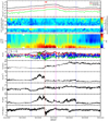 |
Fig. 1. CIR-related proton flux enhancements identified at STEREO-A from 21 to 24 August 2016. Shown from top to bottom are the hourly 1.8–10.0 MeV nucleon−1 proton fluxes, a proton anisotropy plot composed of 1.8–3.6 MeV nucleon−1 proton intensities from 16 different viewing directions of the LET instrument, suprathermal electron PADs, one-minute-averaged magnetic field B, solar wind bulk speed Vp, proton number density Np, proton temperature Tp, total pressure Pt and east–west flow angle. The CIR is highlighted by two blue vertical lines (14:00 UT on 21 August and 10:30 UT on 24 August). The red vertical dashed line presents the passage of the SI (10:09 UT on 22 August) and the magenta vertical line shows the peak values of proton fluxes (03:00 UT on August 23). |
Figure 1 illustrates that the forward and reverse shock were not observed locally and the energetic proton fluxes with different energies peak in the vicinity of the SI. The proton anisotropy plot between the two blue vertical lines shows the approximate isotropic distribution of 1.8–3.6 MeV nucleon−1 protons. It is generally believed that the protons accelerated by distant corotating shocks then propagating back to 1 AU exhibit strong anisotropy, and particles with low energy are modulated significantly by adiabatic deceleration. Therefore, instead of protons being accelerated by the shock at a distance of several astronomical units (AU), there are some mechanisms for local acceleration.
It is generally recognized that the presence of close magnetic structures, such as reconnecting current sheets, magnetic islands, or flux ropes produced by turbulence and large- or small-scale turbulent magnetic reconnection, manifests as IMF directional changes and the formation of two “stripes” in the electron PADs, which is a signature of the strahl electrons propagating along a closed magnetic structure not necessarily connected to a coronal source (Khabarova et al. 2016; Khabarova & Zank 2017; Adhikari et al. 2019). However, there are not two obvious stripes in the PAD of electrons from Fig. 1, which means that the “sea” of magnetic islands may not have formed to trap and accelerate energetic protons that are pre-accelerated at reconnecting current sheets. In addition, the theoretical model and event analysis (Zank et al. 2015; Khabarova & Zank 2017; Zhao et al. 2018; Adhikari et al. 2019; Le Roux et al. 2019) of local particle acceleration related to magnetic islands in the solar wind confirm that the order of the flux amplification factor relative to the reconnection exhausts increases with increasing energy. However, the fact that the evolution of proton fluxes with different energies in Fig. 1 behaves similarly illustrates that the event does not follow the rule, which also demonstrates that the local acceleration mechanism associated with magnetic islands may not be able to explain the flux enhancements. Therefore, we focus on the mechanism acting in the gradual compression region and create simulations in order to verify whether or not this mechanism could be responsible for flux enhancements of 1.8–10.0 MeV nucleon−1 protons.
3. Model description
In this section, we present our model. We combine a data-driven analytical background model providing solar wind configuration with a particle transport model in order to simulate energetic particle propagation in the interplanetary medium.
3.1. Data-driven background model
Based on the model of Tasnim et al. (2018), we constructed the solar wind configuration. In the model, we restrict attention to the (r, ϕ) plane of a spherical coordinate system and assume θ = 90°. Assuming that θ components are negligible in the (r, ϕ) plane, the fluid motion V and magnetic field B only have nonzero r and ϕ components, which is typical of analytical models (Florens et al. 2007; Schulte in den Bäumen et al. 2011, 2012; Tasnim & Cairns 2016). However, this assumption is not always appropriate; for example, the north–south component of B or Bθ is important for studying the effect of the Earth’s magnetic field on the solar wind and Vθ is often large in coronal mass ejection (CME) events.
The model combines ideal MHD equations for conservation of mass and angular momentum, Gauss’s law for magnetism, and Faraday’s law with an accelerating Vr profile for an isothermal wind. These equations can be expressed as follows:
![$$ \begin{aligned}&\frac{\partial \boldsymbol{L}}{\partial {t}}+\boldsymbol{r}\times \nabla \cdot \left[\left(p+\frac{B^2}{2\mu _0}\right)\boldsymbol{I}+\rho \boldsymbol{V}\boldsymbol{V}-\frac{\boldsymbol{B}\boldsymbol{B}}{\mu _0}\right] =\rho \boldsymbol{r}\times \frac{GM_\odot \boldsymbol{r}}{r^2} ,\end{aligned} $$](/articles/aa/full_html/2024/02/aa47248-23/aa47248-23-eq2.gif)

Equation (1) describes the conservation of mass, where ρ = Nm is the proton mass density, N is the proton number density, and m is the proton mass. In Eq. (2), L = ρr × V is the angular momentum and we assume that the thermal and magnetic pressure (p + B2/(2μ0))I are radially symmetric. Equation (3) represents Gauss’s law for magnetism. Equation (4) shows Faraday’s law with frozen-in approximation. Equation (5) (Parker 1958) is a time-independent equation of fluid motion in view of approximately isothermal solar wind and unimportant magnetic terms of solar wind acceleration, where Cs represents the sound speed.
In our model, we make the assumption that the sources of solar wind are constant over a solar rotation period T = 2π/Ω = 27 days, where Ω is the angular speed of solar rotation, which means that the solar wind quantities are spatially variable but time-stationary in the rotating frame. In other words, there is no intrinsic time variation for an observer rotating with the Sun, but for the noncorotating observers, such as the Earth or STEREO, the observed quantities are time-dependent. We assume that the solar wind quantities depend on r and ϕ in general and are constant for limited ϕ. According to Eqs. (1)–(4), we can derive the expressions of Br(r, ϕ), Bϕ(r, ϕ), Vϕ(r, ϕ), N(r, ϕ) in the inertial frame (more details can be found in Appendix A and Tasnim et al. 2018):
![$$ \begin{aligned}&B_\phi (r,\phi )=\frac{[V_\phi (r,\phi )-\Omega {r}]B_{\rm r}(r,\phi )}{V_{\rm r}(r,\phi )} ,\end{aligned} $$](/articles/aa/full_html/2024/02/aa47248-23/aa47248-23-eq7.gif)
![$$ \begin{aligned}&V_\phi (r,\phi ) =\frac{[\Omega {r}^2-R_{\rm s}V_\phi (R_{\rm s},\phi _{\rm s})]{M_{\rm A}}^2(r,\phi )}{r[1-{M_{\rm A}}^2(r,\phi )]} \nonumber \\&\qquad \qquad +\frac{R_{\rm s}V_{\rm r}(r,\phi )B_\phi (R_{\rm s},\phi _{\rm s})}{rB_{\rm r}(r,\phi )[1-{M_{\rm A}}^2(r,\phi )]}+\Omega {r} ,\end{aligned} $$](/articles/aa/full_html/2024/02/aa47248-23/aa47248-23-eq8.gif)
where (Rs, ϕs) is a point of inner boundary and  is the square of the radial Alfvénic Mach number. With the application of measurement data obtained at the specific position (Rob, ϕob), the quantities at (Rs, ϕs) of the inner boundary can be derived as follows:
![$$ \begin{aligned}&B_\phi (R_{\rm s},\phi _{\rm s})=\frac{[V_\phi (R_{\rm s},\phi _{\rm s})-\Omega {R_{\rm s}}]B_{\rm r}(R_{\rm s},\phi _{\rm s})}{V_{\rm r}(R_{\rm s},\phi _{\rm s})} ,\end{aligned} $$](/articles/aa/full_html/2024/02/aa47248-23/aa47248-23-eq12.gif)
![$$ \begin{aligned}&V_\phi (R_{\rm s},\phi _{\rm s})=\frac{(\Omega {{R_{\rm A}}^2}-\Omega {{R_{\rm s}}^2})B_{\rm r}(R_{\rm A},\phi _{\rm A})V_{\rm r}(R_{\rm s},\phi _{\rm s})}{R_{\rm s}[V_{\rm r}(R_{\rm s},\phi _{\rm s})B_{\rm r}(R_{\rm A},\phi _{\rm A})-V_{\rm r}(R_{\rm A},\phi _{\rm A})B_{\rm r}(R_{\rm s},\phi _{\rm s})]} ,\end{aligned} $$](/articles/aa/full_html/2024/02/aa47248-23/aa47248-23-eq13.gif)
where MA(RA, ϕA) = 1 at the position (RA, ϕA) and RA is the Alfvénic critical radius.
According to Eq. (5), the accelerating solar wind solution can be expressed as (Cranmer 2004)
![$$ \begin{aligned} {V_{\rm r}}^2(r,\phi )=\left\{ \begin{array}{ll} -{C_{\rm s}}^2(\phi )W_0[-D(r,\phi )],&r\le {R_{\rm so}(\phi ),} \\ -{C_{\rm s}}^2(\phi )W_{-1}[-D(r,\phi )],&r>R_{\rm so}(\phi ), \\ \end{array} \right. \end{aligned} $$](/articles/aa/full_html/2024/02/aa47248-23/aa47248-23-eq15.gif)
where D(r, ϕ) = [r/Rso(ϕ)]−4exp[4(1 − Rso(ϕ)/r)−1]; Vr(Rso, ϕ) = Cs(ϕ) at the sonic point ![$ R_{\rm so}(\phi)=GM_\odot/[2{C_{\rm s}}^2(\phi)] $](/articles/aa/full_html/2024/02/aa47248-23/aa47248-23-eq16.gif) ; and W0(x) and W−1(x) are two real branches of the Lambert W function (more details can be found in Appendix B).
; and W0(x) and W−1(x) are two real branches of the Lambert W function (more details can be found in Appendix B).
As solar rotation causes the ϕ coordinate to vary with r and time t, the quantities r, Rs, ϕ, ϕs, t and start time t0 of the period [t0, t0 + T] when the longitude meridian ϕs = 0 faces the spacecraft are related by (Florens et al. 2007)


where Vav is the average radial solar wind speed Vr(r, ϕ) over R and T, which is used in order to prevent the streamlines from crossing and R = Rob − Rs.
For the present study, we used the hourly measurement data in a heliocentric radial-tangential-normal (RTN) system obtained by STEREO-A from 31 July to 26 August 2016 in order to construct the 2D solar wind background. In order to reduce the variabilities in the measurements, we performed an 11 hour sliding average of the plasma and magnetic field data. We chose the inner boundary Rs = 10 R⊙, where R⊙ is the solar radius, and Rob ≈ 1 AU. Figure 2 shows the distribution of Vr and N* = N(r/Rob)2 as functions of r and ϕ within 1 AU (panels a and b) and within 5 AU (panels c and d) at 31 July 00:00 UT. The solar wind background rotates counterclockwise over time. The stationary observer (STEREO-A) shown by a red filled circle is at (X, Y) ≈ (1 AU,0). The magnetic field lines shown by solid black lines with arrows illustrate non-Parker spiral behavior and the CIR region concerned is constructed and identified by a magenta line in Fig. 2. The 2D data-driven model can predict the large-scale stable solar wind structure, but the magnetic field evolution and solar wind physics are not included in the model (Tasnim et al. 2019).
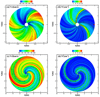 |
Fig. 2. 2D constructed solar wind configuration at 31 July 00:00 UT obtained by the data-driven background model. The Sun is at (X, Y) = (r cos ϕ, r sin ϕ) = (0, 0) and the stationary observer (STEREO-A) marked by a red filled circle is at (X, Y)≈(1, 0). The solar wind background rotates counterclockwise over time. Panels a and b: Vr(r, ϕ) and N*(r, ϕ) = N(r, ϕ)(r/Rob)2 within 1 AU and the studied CIR region identified by the magenta line. Panels c and d: Vr(r, ϕ) and N*(r, ϕ) within 5 AU. |
Figure 3 shows the results at 1 AU from the background model (red lines) and hourly measurement data accessed from STEREO-A (black lines) from 31 July to 26 August 2016 (648 h in total). With the application of the measurement data mentioned in the expressions of solar wind quantities, the predicted data agree well with the actual solar wind parameter values. The physical variables in the blue shaded region are related to the CIR structure being studied here. Because the measurement data entered into the model are a sliding average, there is no obvious current sheet or shock structure in the simulated CIR region related to the energetic particle event, and so we pay attention to the effect of the mechanism acting in the compression region on the flux enhancements.
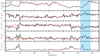 |
Fig. 3. Results at 1 AU from the background model (red lines) and hourly measurement data obtained by STEREO-A (black lines) from 31 July to 26 August 2016 (648 h in total). From top to bottom: radial component of solar wind velocity Vr, magnetic field component Br, Bϕ, magnetic field strength B, and proton number density N. The solar wind variables related to the CIR structure being studied are marked by the blue shaded region. |
3.2. Particle transport model
The transport of energetic particles in the interplanetary medium can be expressed by the focused transport equation (FTE) written in mixed frames (Skilling 1971; Qin et al. 2006; Zhang et al. 2009):

with

![$$ \begin{aligned}&\frac{\mathrm{d} p}{\mathrm{d} t}=-p \left[\frac{(1-\mu ^2)}{2}(\nabla \cdot \boldsymbol{V}-\boldsymbol{b}\boldsymbol{b}:\nabla \boldsymbol{V})+\mu ^2\boldsymbol{b}\boldsymbol{b}:\nabla \boldsymbol{V}\right]-\frac{\mu {p}}{v}\boldsymbol{b}\cdot \frac{\mathrm{d} \boldsymbol{V}}{\mathrm{d} t} , \end{aligned} $$](/articles/aa/full_html/2024/02/aa47248-23/aa47248-23-eq21.gif)
where f(x, μ, p, t) is the gyrophase-averaged distributed function; x is the position in a heliographic inertial coordinate; μ, p, and v are the particle pitch-angle cosine, momentum, and speed, respectively, in the solar wind frame; t is the time; b is the unit magnetic field vector; V is the solar wind velocity; LB = −(b ⋅ ∇lnB)−1 is the magnetic field focusing length in the nonuniform ambient interplanetary magnetic field B; Dμμ is the pitch angle diffusion coefficient; and κ⊥ is the spatial perpendicular diffusion tensor. The FTE includes important particle transport effects, such as particle streaming along the magnetic field lines, adiabatic cooling in the expanding solar wind, magnetic focusing in the diverging IMF, and spatial diffusion caused by magnetic turbulence with respect to the IMF.
Here, the pitch angle diffusion coefficient is set as (Beeck & Wibberenz 1986; Qin et al. 2005)
\cos ^2\psi ,\end{aligned} $$](/articles/aa/full_html/2024/02/aa47248-23/aa47248-23-eq22.gif)
where the constant D0 represents the magnetic field fluctuation level and is obtained by setting the radial mean free path of 100 MeV nucleon−1 proton λ0 as a constant (Bieber et al. 1994); the constant q = 5/3 indicates a Kolmogorov spectrum of magnetic field turbulence in the inertial range; the constant h = 0.2 is added to describe the nonlinear effect of scattering through μ = 0; and ψ denotes the angle between the radial and the IMF direction.
To describe the motion of particles perpendicular to the IMF, the diffusion tensor is chosen as (Wijsen et al. 2019a,b)
where λ|| is the particle parallel mean free path; the relation between the radial mean free path λr and λ|| is λr = λ||cos2ψ; α is a free parameter that denotes the ratio of perpendicular to parallel diffusion coefficient κ⊥/κ|| at a reference magnetic strength B0, and κ|| = vλ||/3. The parallel free path is defined as (Jokipii 1966; Earl 1974)
We use a time-backward method of simulating stochastic processes to solve Eq. (17) numerically (Qin et al. 2006; Zhang et al. 2009). We assume that source particles with a power-law spectrum γ0 = 5.0 are injected at the inner boundary Rin. The inner boundary condition of Eq. (17) can be expressed as

where Ek is source particle’s kinetic energy; τc and τl are time constants controlling the time profile of released particles. We adopt the scenario where the origin of the seed particles occurs in multiple micro- and nanoflares, and assume that they are uniformly distributed at the inner boundary Rin (Wijsen et al. 2023), which means a(ϕ) = 1 in Eq. (23). The FTE (Eq. (17)) can be derived from the guiding center theory and the motion of particles can be considered as the motion of guiding center along the magnetic field line plus the pitch angle diffusion and perpendicular diffusion (Zhao et al. 2016). Based on the 2D solar wind model in Sect. 3.1, we are mainly concerned with the transport of particles on the (r, ϕ) plane of a spherical coordinate system, and so we add δ(θ − 90° ) into Eq. (23) to restrict the injection of particles to the (r, ϕ) plane. Moreover, we assume Eq. (23) is independent of time and fb(x, μ, p, t)|r = Rin can be considered as fb(x, μ, p)|r = Rin, which is more compatible with the scenario where the population of seed particles originates from multiple micro- and nanoflares (Wijsen et al. 2023).
With the outer boundary as an absorptive boundary at Rout, the exact solution of Eq. (17) is the expectation value of the inner boundary at the exit point (xe, μe, pe; Zhang et al. 2009):
where xe, μe, and pe are parameters when the stochastic trajectories hit the inner boundary and N is the total number of injected particles.
3.3. Model coupling
The data-driven background model provides the 2D interplanetary solar wind configuration that is then used by the particle model to simulate energetic particle propagation in the interplanetary space. Here we present a brief description of how the models are coupled.
The solar wind quantities are time-dependent in the inertial frame and the trajectories of particles also depend on time; therefore, we need the background at each time step to coincide with the particle transport model. For example, if we define the solar wind pattern in Fig. 2 as the solar wind configuration at the moment t = 0, where t is time, and the initial backward time s = 0 at the moment t = t1, the solar wind background should rotate counterclockwise with time until t = t1 − Δt when particles run backward with backward time s = Δt (Zhang et al. 2009; Wei et al. 2019).
The simulated domain in the background model is 10 R⊙ ≤ r ≤ 5.5 AU and 0 ≤ ϕ < 2π on a numerical grid. For the particle transport model, we set the inner boundary at Rin = 0.1 AU and the outer boundary at Rout = 5 AU, which is far enough for calculating the particle intensity near 1 AU. Noting that particles propagate in a grid-free numerical scheme, we interpolate the solar wind quantities to the locations of particles at each time step by use of bilinear interpolation.
4. Results and discussion
In this section, we discuss the enhancements in 1.8–10 MeV nucleon−1 proton fluxes observed from 21 to 24 August 2016 by STEREO-A. First, we set the free parameter α = 0, which means the perpendicular diffusion is not included. For our simulation, we injected N0 = 107 protons at the location of the stationary observer with an initial pitch angle cosine μ uniformly distributed between −1 and 1. The proton energy channels were chosen as 1, 5, and 10 MeV nucleon−1. We set λ0 = 1.0 AU, which meant the radial mean paths λr of 1, 5, and 10 MeV nucleon−1 protons were 0.212, 0.362, and 0.457 AU, respectively. In Fig. 4, we plot the flux  and the anisotropy
  . We see that for three energy channels, the fluxes begin to rise obviously at 538 h and maintain a maximum between 543 h and 549 h, while the anisotropies approaching zero indicates that the distribution of protons is nearly isotropic. The red vertical line shows the passage of the SI and the peaks of flux are in the vicinity of the SI.
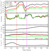 |
Fig. 4. Temporal evolution of different energy proton fluxes, anisotropies, solar wind velocity, magnetic field, and proton number density. The fluxes and anisotropies of protons are from the simulation without perpendicular diffusion and the solar wind parameters are derived from the CIR structure. The red vertical line shows the passage of the SI and the moment of measured flux maximum represented by the magenta vertical line. |
Without perpendicular diffusion, it is generally believed that particles move and diffuse along magnetic field lines. As there is no shock structure in the generated solar wind configuration, and no other accelerating sources are included in the model, we focus our discussion on the transport effects of protons in the compression region. Previous studies showed that the adiabatic cooling effect could change the total fluxes rather than alter the enhancement pattern in the compression region (Wei et al. 2019) and our simulation results (not shown here) confirm this conclusion. The distribution of protons tends to be isotropic during the period related to simulated flux maximum in Fig. 4, which illustrates that the mechanisms associated with the variation of the pitch angle μ are notable. The variation of μ over backward time s is described as follows:
![$$ \begin{aligned}&\mathrm{d} \mu (s)=\sqrt{2\max (D_{\mu \mu },0)}\mathrm{d} w(s)+\left[\frac{\partial {D_{\mu \mu }}}{\partial {\mu }}-\frac{\left(1-\mu ^2(s)\right)v}{2L_{\rm B}}\right.\nonumber \\&\ \ \qquad -\frac{\mu (s)(1-\mu ^2(s))}{2}(\nabla \cdot \boldsymbol{V}-3\boldsymbol{b}\boldsymbol{b}:\nabla \boldsymbol{V}) \nonumber \\&\ \ \qquad \left.+\frac{(1-\mu ^2(s))}{v}\boldsymbol{b}\cdot \frac{\mathrm{d} \boldsymbol{V}}{\mathrm{d} t}\right]\mathrm{d} s. \end{aligned} $$](/articles/aa/full_html/2024/02/aa47248-23/aa47248-23-eq29.gif)
In Eq. (25), dw(s) is a Wiener process and the final term is much smaller than other transport effects. We now discuss the magnetic focusing effect related with LB and the effect of pitch-angle diffusion –represented by Dμμ– on the flux enhancements. We present protons with energies of 5 MeV nucleon−1 as an example in Fig. 5. The variation in reciprocal magnetic focusing length (LB)−1 can describe the strength of the magnetic focusing effect (Giacalone et al. 2002). Panel a shows the results obtained by altering the variation of (LB)−1 compared to the original (LB)−1, where (LB)−1 ∼ 547 and (LB)−1 ∼ 560 demonstrate that the strength of the magnetic focusing effect for particles propagating along different magnetic field lines is the same as that for the field line magnetically connected to the observer at 547 h and 560 h, respectively. Panel b shows the effect of pitch-angle diffusion by setting different values of λ0, where λ0 = 0.5, 1.5, and 3.0 AU, corresponding to the radial mean free paths λr of 5 MeV nucleon−1 protons are 0.181, 0.554, and 1.087 AU, respectively. This indicates that the variation in the strength of the magnetic focusing effect is responsible for the evolution of proton fluxes and the effect of pitch-angle diffusion influences the total flux.
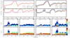 |
Fig. 5. Effect of magnetic focusing and pitch-angle diffusion of 5 MeV nucleon−1 proton propagation on flux enhancements. Panel a: results obtained by altering the strength of the magnetic focusing effect described by the variation of (LB)−1. Panel b: effect of pitch-angle diffusion by setting different values of λ0. Panels c–f: contour plots of log[G(pe; x, μ, p, t)] and log[G(pe; x, μ, p, t)fb(xe, pe, μe)/f(x, μ, p, t)] as functions of source particle momentum pe/p and observation time. |
If we bin the values inside Eq. (24) by source particle momentum pe, then the solution to the FTE can be expressed as follows (Zhang et al. 2009):
where G(pe; x, μ, p, t) can be considered as a backward Green’s function. In Eq. (26), the product G(pe; x, μ, p, t)fb(xe, pe, μe) is the true distribution of source particles for those observed at (x, μ, p, t) and G(pe; x, μ, p, t)fb(xe, pe, μe)/f(x, μ, p, t) represents the contribution of different momentum source particles to the solution. Panels c–f in Fig. 5 show the contour plots of log[G(pe; x, μ, p, t)] and log[G(pe; x, μ, p, t)fb (xe, pe, μe)/f(x, μ, p, t)] as functions of source particle momentum pe/p and observation time.
Panel c shows that the backward Green’s function is bigger and the momentum distribution of source particles is wider during the period related to maximum flux, which illustrates that the magnetic field structure can trap more protons that then undergo multiple acceleration and deceleration. As shown in panel d, the backward Green’s function and the momentum distribution of source particles corresponding to different observation time are close to each other when the variation in the strength of the magnetic focusing effect for particle propagating along different magnetic field lines is the same as that for the field line magnetically connected to the observer at 560 h, which brings a gently varying flux profile. On the other hand, the occurrence of small or even negative (LB)−1 values in the compression region emphasizes the local focusing or mirroring effect (Kocharov et al. 2003; Wei et al. 2019) and more particles will be scattered back and forth when they encounter strong magnetic mirrors. Figure 6 provides radial variations of [LB(r, ϕ)]−1 for field lines magnetically connected to the observer at 547 h and 560 h. It is obvious that smaller (LB)−1 – especially within 1 AU – associated with 547 h demonstrates that the strength of the magnetic mirroring effect is stronger, which leads to more protons being trapped and is related to a larger flux. Panels e and f suggest that more protons will be confined by the trap-like structures of IMF when the free paths of protons get larger. The competition between the effect of pitch-angle diffusion and the magnetic focusing effect can be expressed by the ratio of mean free path to magnetic focusing length λ||/LB (Kocharov et al. 2003; Wei et al. 2019). For the constructed solar wind background, the increase in free path λ|| is equivalent to the increase in ratio λ||/LB, indicating the reduction in effect of pitch-angle diffusion and the promotion in magnetic focusing effect of proton transport.
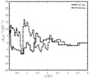 |
Fig. 6. Radial variations of reciprocal magnetic focusing length [LB(r, ϕ)]−1 for the field lines magnetically connected to the observer at 547 h and 560 h. |
However, the simulated proton flux profiles present drastic variation, which is at odds with the measurement data shown in Fig. 1. Therefore, we now consider the effect of perpendicular diffusion. We set λ0 = 1.0 AU and the free parameter α = 0.025, 0.02, and 0.018 for 1, 5, and 10 MeV nucleon−1 protons, respectively. Figure 7 shows the relative fluxes of different energy channels and solar wind quantities from the measurement data (dashed lines) and simulated results (solid lines). In order to examine the temporal evolution of flux, we normalized the fluxes of different energy channels so that they have a relative flux of 1 on 20 August 19:00 UT. The simulated particle fluxes are enhanced gradually by an order of magnitude to reach the maximum values in the vicinity of the SI; they then decay at a similar rate, which is well correlated with the actual flux evolution. With perpendicular diffusion, it is known that there are two phenomena: the gain of particles arriving at the magnetic field line connected to the observer from nearby field lines and the loss of particles from the observer’s magnetic field line (Wang et al. 2012). Due to higher particle speeds and typically larger parallel mean free paths, it is intelligible that high-energy particles are able to diffuse further normal to magnetic field lines with the same ratio α of perpendicular to parallel diffusion coefficient (Wang et al. 2014). Therefore, with the ratio α being larger for the lower energy protons, the flux profiles show a similar trend of gradual variation for different energy protons.
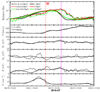 |
Fig. 7. Temporal evolution of relative fluxes and solar wind quantities from measurement data (dashed lines) and simulated results (solid lines). The red vertical line shows the passage of the SI and the magenta vertical line presents the measured flux peaks. |
As shown in Figs. 4 and 7, there is a time difference between the maximum values of fluxes from the simulation and the measurement, where the measured flux peaks are represented by a magenta vertical line. On the other hand, due to the sliding average of measurement data input into the data-driven background model, discontinuous structures in the solar wind, such as the SI, are smoothed and its role as a diffusion barrier is weakened (Wijsen et al. 2019a,b), which causes the simulated flux to be enhanced earlier than that obtained by STEREO-A.
Figure 8 presents the flux peak energy spectra and the event-integrated energy spectra calculated by integrating proton fluxes from 21 August 05:00 UT to 24 August 10:00 UT. The solid and dashed lines illustrate the power-law fit to the spectra. It is noticeable that the estimated spectrum indexes from the simulation are in good agreement with those from measurements, regardless of whether they are deduced from the peak or event-integrated spectra. Although there are some distinctions between the characteristics of the simulated flux profiles and the measured ones, we believe that the magnetic focusing effect of particle propagation in the compression region plays an important role in the energetic particle event. In other words, the mechanism of particle scattering back and forth between the trap-like structure of the IMF in the compression region is the major driver of the flux enhancements of 1.8–10.0 MeV nucleon−1 protons.
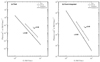 |
Fig. 8. Measured (circles) and simulated (asterisks) energy spectra of energetic protons. The solid and dashed lines illustrate the power-law fit to the spectra. Panel a: flux peak energy spectra, where the estimated spectrum indexes are 3.68 from the simulation and 3.38 from the measurement. Panel b: event-integrated energy spectra calculated by integrating proton fluxes from 21 August 05:00 UT to 24 August 10:00 UT and the spectrum indexes are 3.62 and 3.45, respectively. |
5. Conclusion
In this paper, we examined a CIR-related energetic particle event measure by STEREO-A from 21 to 24 August 2016. From the analysis of measurement data, we suggest that certain mechanisms of local acceleration drive the flux enhancements of 1.8–10.0 MeV nucleon−1 protons rather than distant shock acceleration. In order to validate our hypothesis that a local mechanism acting in the gradual compression region plays a crucial role in the energetic particle event, we developed a coupled model to simulate energetic proton transport in a simple but more realistic solar wind background.
The coupled model is composed of a data-driven 2D analytical solar wind model and a particle transport model. The background model driven by plasma and magnetic field data from STEREO-A provides the solar wind density, velocity, and magnetic field as functions of r and ϕ in a spherical polar coordinate system. Also, a time-backward Markov stochastic method is used to solve the FTE that describes particle transport in the interplanetary space.
First, we did not include the effect of perpendicular diffusion and restricted attention to the transport effects of protons in the compression region without any other accelerating sources. We find that the variation in the strength of the local mirroring effect can alter the flux pattern, while the effect of pitch-angle diffusion influences the flux level. These findings are consistent with the conclusions of Wei et al. (2019). The simulated results illustrate that the magnetic field configuration in the vicinity of SI can trap more particles – that undergo multiple acceleration and deceleration –, which brings an obvious rise in flux.
Subsequently, we set the ratio of perpendicular to parallel diffusion coefficient κ⊥/κ|| = α ∼ 10−2, similar to Dröge et al. (2010), in order to calculate the relative fluxes and derive the energy spectra. With perpendicular diffusion, the temporal evolution of simulated fluxes is consistent with that of measurement data. Although the occurrence of simulated flux peaks and the enhancements of simulated fluxes are earlier than those from STEREO-A, the estimated spectrum indexes from simulations are in good agreement with those from measurements, regardless of whether they are deduced from the peak or event-integrated spectra.
From our analysis of simulated results, we believe that the local mechanism of particle scattering back and forth within the trap-like structure of the IMF in the gradual compression region is the main driver of the energetic particle event, and that perpendicular diffusion plays an important role in the temporal evolution of proton fluxes. Our simulation results are well correlated with the measurement data.
It should be pointed out that the measurement data required to initialize the solar wind model are not limited to those that come from STEREO or other spacecraft near 1 AU, such as WIND and ACE. The solar wind background and energetic particle distribution predicted using the coupled model above with data from Parker Solar Probe, Beppi-Colombo, and Solar Orbiter inside 1 AU or from Mars Atmosphere and Volatile Evolution (MAVEN) and Tianwen-1 outside 1 AU will help us to understand the transport and acceleration of energetic particles and the evolution of the solar wind configuration more comprehensively, and this will be the focus of our future work.
Acknowledgments
The data for this work are provided by the STEREO Science Center (https://stereo-ssc.nascom.nasa.gov/data.shtml) and this research has made use of NASA’s Astrophysics Data System. The work is jointly supported by National Key RD Program of China (Grant Nos. 2022YFF0503800 and 2021YFA0718600), the National Natural Science Foundation of China (42330210, 41974202, 42004146, 42030204 and 42004144), the Strategic Priority Research Program of the Chinese Academy of Sciences, Grant No. XDB 41000000, and the Specialized Research Fund for State Key Laboratories.
References
- Acuña, M. H., Curtis, D., Scheifele, J. L., et al. 2008, Space. Sci. Rev., 136, 203 [CrossRef] [Google Scholar]
- Adhikari, L., Khabarova, O., Zank, G. P., & Zhao, L. L. 2019, ApJ, 873, 72 [Google Scholar]
- Allen, R. C., Lario, D., Odstrcil, D., et al. 2020, ApJS, 246, 36 [Google Scholar]
- Beeck, J., & Wibberenz, G. 1986, ApJ, 311, 437 [NASA ADS] [CrossRef] [Google Scholar]
- Bieber, J. W., Matthaeus, W. H., Smith, C. W., et al. 1994, ApJ, 420, 294 [Google Scholar]
- Chen, J. H., Schwadron, N. A., Möbius, E., & Gorby, M. 2015, J. Geophys. Res. Space Phys., 120, 9269 [Google Scholar]
- Chotoo, K., Schwadron, N. A., Mason, G. M., et al. 2000, J. Geophys. Res., 105, 23107 [Google Scholar]
- Cranmer, S. R. 2004, Am. J. Phys., 72, 1397 [NASA ADS] [CrossRef] [Google Scholar]
- Desai, M. I., Mitchell, D. G., Szalay, J. R., et al. 2020, ApJS, 246, 56 [Google Scholar]
- Dröge, W., Kartavykh, Y. Y., Klecker, B., & Kovaltsov, G. A. 2010, ApJ, 709, 912 [CrossRef] [Google Scholar]
- Dwyer, J. R., Mason, G. M., Mazur, J. E., et al. 1997, ApJ, 490, L115 [NASA ADS] [CrossRef] [Google Scholar]
- Earl, J. A. 1974, ApJ, 193, 231 [NASA ADS] [CrossRef] [Google Scholar]
- Ebert, R. W., Dayeh, M. A., Desai, M. I., & Mason, G. M. 2012, ApJ, 749, 73 [Google Scholar]
- Fisk, L. A., & Lee, M. A. 1980, ApJ, 237, 620 [Google Scholar]
- Florens, M. S. L., Cairns, I. H., Knock, S. A., & Robinson, P. A. 2007, Geophys. Res. Lett., 34, L04104 [NASA ADS] [CrossRef] [Google Scholar]
- Galvin, A. B., Kistler, L. M., Popecki, M. A., et al. 2008, Space. Sci. Rev., 136, 437 [NASA ADS] [CrossRef] [Google Scholar]
- Giacalone, J., Jokipii, J. R., & Kóta, J. 2002, ApJ, 573, 845 [Google Scholar]
- Jian, L., Russell, C. T., Luhmann, J. G., & Skoug, R. M. 2006, Sol. Phys., 239, 337 [NASA ADS] [CrossRef] [Google Scholar]
- Jokipii, J. R. 1966, ApJ, 146, 480 [Google Scholar]
- Joyce, C. J., McComas, D. J., Schwadron, N. A., et al. 2021, A&A, 650, L5 [EDP Sciences] [Google Scholar]
- Khabarova, O. V., & Zank, G. P. 2017, ApJ, 843, 4 [NASA ADS] [CrossRef] [Google Scholar]
- Khabarova, O., Zank, G. P., Li, G., et al. 2015, ApJ, 808, 181 [Google Scholar]
- Khabarova, O. V., Zank, G. P., Li, G., et al. 2016, ApJ, 827, 122 [Google Scholar]
- Kocharov, L., Kovaltsov, G. A., Torsti, J., Anttila, A., & Sahla, T. 2003, J. Geophys. Res. Space Phys., 108, 1404 [NASA ADS] [CrossRef] [Google Scholar]
- Kocharov, L., Pizzo, V. J., Odstrcil, D., & Zwickl, R. D. 2009, J. Geophys. Res. Space Phys., 114, A05102 [NASA ADS] [CrossRef] [Google Scholar]
- Kóta, J., & Jokipii, J. R. 2000, ApJ, 531, 1067 [Google Scholar]
- Le Roux, J. A., Webb, G. M., Khabarova, O. V., Zhao, L. L., & Adhikari, L. 2019, ApJ, 887, 77 [NASA ADS] [CrossRef] [Google Scholar]
- Luhmann, J. G., Curtis, D. W., Schroeder, P., et al. 2008, Space. Sci. Rev., 136, 117 [NASA ADS] [CrossRef] [Google Scholar]
- Mason, G. M., Mazur, J. E., Dwyer, J. R., Reames, D. V., & von Rosenvinge, T. T. 1997, ApJ, 486, L149 [NASA ADS] [CrossRef] [Google Scholar]
- Mason, G. M., Leske, R. A., Desai, M. I., et al. 2008, ApJ, 678, 1458 [Google Scholar]
- Matthaeus, W. H., Qin, G., Bieber, J. W., & Zank, G. P. 2003, ApJ, 590, L53 [Google Scholar]
- Mewaldt, R. A., Cohen, C. M. S., Cook, W. R., et al. 2008, Space. Sci. Rev., 136, 285 [NASA ADS] [CrossRef] [Google Scholar]
- Parker, E. N. 1958, ApJ, 128, 664 [Google Scholar]
- Qin, G., & Shalchi, A. 2012, Adv. Space Res., 49, 1643 [NASA ADS] [CrossRef] [Google Scholar]
- Qin, G., Zhang, M., Dwyer, J. R., Rassoul, H. K., & Mason, G. M. 2005, ApJ, 627, 562 [NASA ADS] [CrossRef] [Google Scholar]
- Qin, G., Zhang, M., & Dwyer, J. R. 2006, J. Geophys. Res. Space Phys., 111, A08101 [NASA ADS] [CrossRef] [Google Scholar]
- Richardson, I. G., Barbier, L. M., Reames, D. V., & von Rosenvinge, T. T. 1993, J. Geophys. Res., 98, 13 [NASA ADS] [CrossRef] [Google Scholar]
- Sauvaud, J. A., Larson, D., Aoustin, C., et al. 2008, Space. Sci. Rev., 136, 227 [NASA ADS] [CrossRef] [Google Scholar]
- Schulte in den Bäumen, H., Cairns, I. H., & Robinson, P. A. 2011, Geophys. Res. Lett., 38, L24101 [Google Scholar]
- Schulte in den Bäumen, H., Cairns, I. H., & Robinson, P. A. 2012, J. Geophys. Res. Space Phys., 117, A10104 [CrossRef] [Google Scholar]
- Skilling, J. 1971, ApJ, 170, 265 [NASA ADS] [CrossRef] [Google Scholar]
- Tasnim, S., & Cairns, I. H. 2016, J. Geophys. Res. Space Phys., 121, 4966 [NASA ADS] [CrossRef] [Google Scholar]
- Tasnim, S., Cairns, I. H., & Wheatland, M. S. 2018, J. Geophys. Res. Space Phys., 123, 1061 [NASA ADS] [CrossRef] [Google Scholar]
- Tasnim, S., Cairns, I. H., Li, B., & Wheatland, M. S. 2019, Sol. Phys., 294, 155 [NASA ADS] [CrossRef] [Google Scholar]
- Wang, Y., & Qin, G. 2015, ApJ, 806, 252 [NASA ADS] [CrossRef] [Google Scholar]
- Wang, Y., Qin, G., & Zhang, M. 2012, ApJ, 752, 37 [CrossRef] [Google Scholar]
- Wang, Y., Qin, G., Zhang, M., & Dalla, S. 2014, ApJ, 789, 157 [NASA ADS] [CrossRef] [Google Scholar]
- Wei, W., Shen, F., Yang, Z., et al. 2019, J. Atm. Sol.-Terr. Phys., 182, 155 [NASA ADS] [CrossRef] [Google Scholar]
- Wijsen, N., Aran, A., Pomoell, J., & Poedts, S. 2019a, A&A, 624, A47 [NASA ADS] [CrossRef] [EDP Sciences] [Google Scholar]
- Wijsen, N., Aran, A., Pomoell, J., & Poedts, S. 2019b, A&A, 622, A28 [NASA ADS] [CrossRef] [EDP Sciences] [Google Scholar]
- Wijsen, N., Li, G., Ding, Z., et al. 2023, J. Geophys. Res. Space Phys., 128, e2022JA031203 [NASA ADS] [CrossRef] [Google Scholar]
- Zank, G. P., le Roux, J. A., Webb, G. M., Dosch, A., & Khabarova, O. 2014, ApJ, 797, 28 [Google Scholar]
- Zank, G. P., Hunana, P., Mostafavi, P., et al. 2015, ApJ, 814, 137 [Google Scholar]
- Zhang, M. 2010, J. Geophys. Res. Space Phys., 115, A12102 [NASA ADS] [Google Scholar]
- Zhang, M., Qin, G., & Rassoul, H. 2009, ApJ, 692, 109 [NASA ADS] [CrossRef] [Google Scholar]
- Zhao, L., Li, G., Ebert, R. W., et al. 2016, J. Geophys. Res. Space Phys., 121, 77 [NASA ADS] [CrossRef] [Google Scholar]
- Zhao, L. L., Zank, G. P., Khabarova, O., et al. 2018, ApJ, 864, L34 [NASA ADS] [CrossRef] [Google Scholar]
Appendix A: Derivation of the data-driven background model
In the inertial frame, the ideal MHD equations can be expressed by Eq.1-Eq.4; we now transform these equations from the 2D inertial frame into a 2D rotating frame. The standard relations between the inertial frame and rotating frame are ϕ′=ϕ − Ωt and r′=r, where the superscript ‘′’ denotes the rotating frame. In the non-relativistic regime, these quantities in the rotating frame and inertial frame are related to:
For simplicity, we omit the superscript representation in the rotating frame, and the following physical quantities are represented in the rotating frame. The MHD equations can be written in the rotating frame as follows:

![$$ \begin{aligned}&\frac{\partial \boldsymbol{L}}{\partial {t}}+\boldsymbol{r}\times \nabla \cdot [(p+\frac{B^2}{2\mu _0})\boldsymbol{I}+\rho \boldsymbol{V}\boldsymbol{V}-\frac{\boldsymbol{B}\boldsymbol{B}}{\mu _0}]\nonumber \\&=\rho \boldsymbol{r}\times \{\frac{GM_\odot \boldsymbol{r}}{r^2}-[\boldsymbol{\Omega }\times (\boldsymbol{\Omega }\times {\boldsymbol{r}})+2\boldsymbol{\Omega }\times {\boldsymbol{V}}]\} , \end{aligned} $$](/articles/aa/full_html/2024/02/aa47248-23/aa47248-23-eq37.gif)

In Eq.A.7, the last term is centrifugal force. We assume the quantities are time-stationary in the rotating frame and θ = 90° in the spherical coordinate system. Moreover, the electric conductivity of plasma is considered to be infinite, which means that Eq.A.9 can be reduced to E = −V × B = 0 with frozen-in approximation. With the assumptions that V and B only have non-zero Vr, Vϕ, Br, and Bϕ components and the solar wind quantities depend on r and ϕ, in a spherical polar coordinate system, Eq.A.6-Eq.A.9 can be written as

We also assume that the quantities are constant for limited ϕ, which means that ∂/∂ϕ = 0 locally. We integrate Eq.A.10-Eq.A.13 to get the following expressions:


where C1(ϕ), C2(ϕ) and C3(ϕ) are integration constants and are functions of ϕ due to the integration over r.
The integration constants in Eq.A.14-Eq.A.17 are applied at the inner boundary (Rs, ϕs), and then Eq.A.14-Eq.A.17 become


We can find the expressions of Br(r, ϕ) and N(r, ϕ) from Eq.A.18 and Eq.A.20:


and we can deduce the expression of Bϕ(r, ϕ) from Eq.A.19 as follows:
![$$ \begin{aligned} B_\phi (r,\phi )&=\frac{[rV_\phi (r,\phi )+\Omega {r^2}-R_sV_\phi (R_s,\phi _s)-\Omega {R_s}^2]{M_A}^2(r,\phi )B_r(r,\phi )}{rV_r(r,\phi )}\nonumber \\&+\frac{R_s}{r}B_\phi (R_s,\phi _s) , \end{aligned} $$](/articles/aa/full_html/2024/02/aa47248-23/aa47248-23-eq54.gif)
where  is the square of the radial Alfvénic Mach number MA(r, ϕ). The expression of Bϕ(r, ϕ) can also be deduced from Eq.A.21, as follows:
Making Eq.A.24 equal to Eq.A.25, we can get the expression of Vϕ(r, ϕ):
where ![$ d_1=\{[\Omega{r^2}-R_sV_\phi(R_s,\phi_s)-\Omega{R_s}^2]{M_A}^2(r,\phi)B_r(r,\phi)+R_sV_r(r,\phi)B_\phi(R_s,\phi_s)\}/[rB_r(r,\phi)] $](/articles/aa/full_html/2024/02/aa47248-23/aa47248-23-eq58.gif) and
and  .
.
A singularity problem arises in Eq.A.26 at the Alfvénic critical radius RA where the radial Alfvénic number MA(RA, ϕA) = 1. To remove the singularity, the denominator d2 and numerator d1 must both vanish at (RA, ϕA) so that we can deduce the expressions of Bϕ(Rs, ϕs) and Vϕ(Rs, ϕs) with Eq.A.25 and Eq.A.26:
![$$ \begin{aligned} V_\phi (R_s,\phi _s)=\frac{(\Omega {R_A}^2-\Omega {R_s}^2)B_r(R_A,\phi _A)V_r(R_s,\phi _s)}{R_s[V_r(R_s,\phi _s)B_r(R_A,\phi _A)-V_r(R_A,\phi _A)B_r(R_s,\phi _s)]} .\end{aligned} $$](/articles/aa/full_html/2024/02/aa47248-23/aa47248-23-eq61.gif)
Simultaneous use of Eq.A.18 and Eq.A.20 with the application of observational data at a specific location (Rob, ϕob) allows us to derive the following expressions:

The above quantities are expressed in the rotating frame, but the actual measurement data are usually given in the inertial frame. With the application of Eq.A.1-Eq.A.5, we can transform Eq.A.22, Eq.A.23, and Eq.A.25-Eq.A.30 into the following in the inertial frame:
![$$ \begin{aligned} B_\phi (r,\phi )=\frac{[V_\phi (r,\phi )-\Omega {r}]B_r(r,\phi )}{V_r(r,\phi )} ,\end{aligned} $$](/articles/aa/full_html/2024/02/aa47248-23/aa47248-23-eq66.gif)
![$$ \begin{aligned} V_\phi (r,\phi )&=\frac{[\Omega {r}^2-R_sV_\phi (R_s,\phi _s)]{M_A}^2(r,\phi )}{r[1-{M_A}^2(r,\phi )]}\nonumber \\&+\frac{R_sV_r(r,\phi )B_\phi (R_s,\phi _s)}{rB_r(r,\phi )[1-{M_A}^2(r,\phi )]}+\Omega {r} , \end{aligned} $$](/articles/aa/full_html/2024/02/aa47248-23/aa47248-23-eq67.gif)
![$$ \begin{aligned} B_\phi (R_s,\phi _s)=\frac{[V_\phi (R_s,\phi _s)-\Omega {R_s}]B_r(R_s,\phi _s)}{V_r(R_s,\phi _s)} ,\end{aligned} $$](/articles/aa/full_html/2024/02/aa47248-23/aa47248-23-eq68.gif)
![$$ \begin{aligned} V_\phi (R_s,\phi _s)=\frac{(\Omega {{R_A}^2}-\Omega {{R_s}^2})B_r(R_A,\phi _A)V_r(R_s,\phi _s)}{R_s[V_r(R_s,\phi _s)B_r(R_A,\phi _A)-V_r(R_A,\phi _A)B_r(R_s,\phi _s)]} ,\end{aligned} $$](/articles/aa/full_html/2024/02/aa47248-23/aa47248-23-eq69.gif)
Appendix B: Solution for the accelerating solar wind
For the accelerating Vr profile of an isothermal solar wind, the time-independent equation of fluid motion is chosen as (Parker 1958):

with the assumption mentioned in Sect.3.1, integrating Eq.B.1 yields Bernoulli integral (Parker 1958):

where C4(ϕ) is the integration constant. Equation B.2 has a transonic solution Vr(r, ϕ) = Cs(ϕ) at the sonic critical radius ![$ R_{so}(\phi)=GM_\odot/[2{C_s}^2(\phi)] $](/articles/aa/full_html/2024/02/aa47248-23/aa47248-23-eq74.gif) , so we can get C4(ϕ) = − 3.
, so we can get C4(ϕ) = − 3.
From Cranmer (2004), the accelerating solar wind solution of Eq.B.2 can be expressed as:
![$$ \begin{aligned} {V_r}^2(r,\phi )=\left\{ \begin{array}{ll} -{C_s}^2(\phi )W_0[-D(r,\phi )],&r\le {R_{so}(\phi )} \\ -{C_s}^2(\phi )W_{-1}[-D(r,\phi )],&r>R_{so}(\phi ) \\ \end{array} \right. ,\end{aligned} $$](/articles/aa/full_html/2024/02/aa47248-23/aa47248-23-eq75.gif)
where D(r, ϕ) = [r/Rso(ϕ)]−4exp[4(1 − Rso(ϕ)/r)−1], W0(x) and W−1(x) are two real branches of Lambert W function.
The crux of acquiring Vr(r, ϕ) profile is the magnitude of Rso(ϕ) or Cs(ϕ). An isothermal wind of ionized hydrogen has constant sound speed Cs(ϕ) for each ϕ. The relation between the radial solar wind speed Vr(Rob, ϕ) at specific location of spacecraft and the sound speed Cs(ϕ) can be obtained empirically (Tasnim et al. 2018):

where k(ϕ) is a free parameter for each ϕ, and usually takes a value of between 3 and 5 for the Vr(Rob, ϕ) at 1 AU. Given that Cs(ϕ) = Vr(Rob, ϕ)/k(ϕ), we can substitute it into Eq.B.3 to obtain the Vr(r, ϕ) profile. In order to minimize the difference between the predicted values of Vr(r, ϕ) at the observation point and the actual observed data Vr(Rob, ϕ), we vary the value of k(ϕ) for each ϕ in each trial to get the best results. The longitudinal variations of k(ϕ) for the period 31 July to 26 August, 2016, which represents 648 hours in total, are presented in Fig.B.1, while the radial variations of Vr are shown in Fig.B.2.
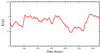 |
Fig. B.1. Temporal or longitudinal variations of k(ϕ) for the period 31 July to 26 August 2016 (648 hours in total). |
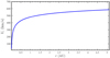 |
Fig. B.2. Radial variations of Vr. |
All Figures
|
Fig. 1. CIR-related proton flux enhancements identified at STEREO-A from 21 to 24 August 2016. Shown from top to bottom are the hourly 1.8–10.0 MeV nucleon−1 proton fluxes, a proton anisotropy plot composed of 1.8–3.6 MeV nucleon−1 proton intensities from 16 different viewing directions of the LET instrument, suprathermal electron PADs, one-minute-averaged magnetic field B, solar wind bulk speed Vp, proton number density Np, proton temperature Tp, total pressure Pt and east–west flow angle. The CIR is highlighted by two blue vertical lines (14:00 UT on 21 August and 10:30 UT on 24 August). The red vertical dashed line presents the passage of the SI (10:09 UT on 22 August) and the magenta vertical line shows the peak values of proton fluxes (03:00 UT on August 23). |
| In the text | |
|
Fig. 2. 2D constructed solar wind configuration at 31 July 00:00 UT obtained by the data-driven background model. The Sun is at (X, Y) = (r cos ϕ, r sin ϕ) = (0, 0) and the stationary observer (STEREO-A) marked by a red filled circle is at (X, Y)≈(1, 0). The solar wind background rotates counterclockwise over time. Panels a and b: Vr(r, ϕ) and N*(r, ϕ) = N(r, ϕ)(r/Rob)2 within 1 AU and the studied CIR region identified by the magenta line. Panels c and d: Vr(r, ϕ) and N*(r, ϕ) within 5 AU. |
| In the text | |
|
Fig. 3. Results at 1 AU from the background model (red lines) and hourly measurement data obtained by STEREO-A (black lines) from 31 July to 26 August 2016 (648 h in total). From top to bottom: radial component of solar wind velocity Vr, magnetic field component Br, Bϕ, magnetic field strength B, and proton number density N. The solar wind variables related to the CIR structure being studied are marked by the blue shaded region. |
| In the text | |
|
Fig. 4. Temporal evolution of different energy proton fluxes, anisotropies, solar wind velocity, magnetic field, and proton number density. The fluxes and anisotropies of protons are from the simulation without perpendicular diffusion and the solar wind parameters are derived from the CIR structure. The red vertical line shows the passage of the SI and the moment of measured flux maximum represented by the magenta vertical line. |
| In the text | |
|
Fig. 5. Effect of magnetic focusing and pitch-angle diffusion of 5 MeV nucleon−1 proton propagation on flux enhancements. Panel a: results obtained by altering the strength of the magnetic focusing effect described by the variation of (LB)−1. Panel b: effect of pitch-angle diffusion by setting different values of λ0. Panels c–f: contour plots of log[G(pe; x, μ, p, t)] and log[G(pe; x, μ, p, t)fb(xe, pe, μe)/f(x, μ, p, t)] as functions of source particle momentum pe/p and observation time. |
| In the text | |
|
Fig. 6. Radial variations of reciprocal magnetic focusing length [LB(r, ϕ)]−1 for the field lines magnetically connected to the observer at 547 h and 560 h. |
| In the text | |
|
Fig. 7. Temporal evolution of relative fluxes and solar wind quantities from measurement data (dashed lines) and simulated results (solid lines). The red vertical line shows the passage of the SI and the magenta vertical line presents the measured flux peaks. |
| In the text | |
|
Fig. 8. Measured (circles) and simulated (asterisks) energy spectra of energetic protons. The solid and dashed lines illustrate the power-law fit to the spectra. Panel a: flux peak energy spectra, where the estimated spectrum indexes are 3.68 from the simulation and 3.38 from the measurement. Panel b: event-integrated energy spectra calculated by integrating proton fluxes from 21 August 05:00 UT to 24 August 10:00 UT and the spectrum indexes are 3.62 and 3.45, respectively. |
| In the text | |
|
Fig. B.1. Temporal or longitudinal variations of k(ϕ) for the period 31 July to 26 August 2016 (648 hours in total). |
| In the text | |
|
Fig. B.2. Radial variations of Vr. |
| In the text | |
Current usage metrics show cumulative count of Article Views (full-text article views including HTML views, PDF and ePub downloads, according to the available data) and Abstracts Views on Vision4Press platform.
Data correspond to usage on the plateform after 2015. The current usage metrics is available 48-96 hours after online publication and is updated daily on week days.
Initial download of the metrics may take a while.