| Issue |
A&A
Volume 690, October 2024
|
|
|---|---|---|
| Article Number | A239 | |
| Number of page(s) | 10 | |
| Section | Astrophysical processes | |
| DOI | https://doi.org/10.1051/0004-6361/202450545 | |
| Published online | 14 October 2024 | |
Fast X-ray/IR observations of the black hole transient Swift J1753.5–0127: From an IR lead to a very long jet lag
1
INAF - IASF Palermo, Via Ugo La Malfa, 153, I-90146 Palermo, Italy
2
Università degli Studi di Palermo, Dipartimento di Fisica e Chimica, Via Archirafi 36, I-90123 Palermo, Italy
3
Instituto de Astrofísica de Canarias, E-38205 La Laguna, Tenerife, Spain
4
Departamento de Astrofísica, Universidad de La Laguna, E-38206 La Laguna, Tenerife, Spain
5
INAF – Osservatorio Astronomico di Roma, Via Frascati 33, I-00078 Monteporzio Catone, Italy
6
Department of Physics and Astronomy, FI-20014 University of Turku, Finland
7
Nordita, Stockholm University and KTH Royal Institute of Technology, Hannes Alfvéns väg 12, SE-10691 Stockholm, Sweden
8
Department of Physics & Astronomy, Texas Tech University, Box 41051 Lubbock, TX 79409-1051, USA
9
Center for Astrophysics and Space Science (CASS), New York University Abu Dhabi, P.O. Box 129188 Abu Dhabi, UAE
10
Anton Pannekoek Institute, University of Amsterdam, Science Park 904, 1098 XH Amsterdam, The Netherlands
11
INAF, Osservatorio Astronomico di Brera, Via E. Bianchi 46, I-23807 Merate (LC), Italy
12
Dipartimento di Fisica, Universita degli Studi di Roma “Tor Vergata”, Via della Ricerca Scientifica 1, I-00133 Rome, Italy
13
University of Oxford, Department of Physics, Astrophysics, Denys Wilkinson Building, Keble Road, OX1 3RH Oxford, UK
14
Centre for Advanced Instrumentation, Department of Physics, Durham University, Durham, UK
15
Dipartimento di Fisica, Università degli Studi di Cagliari, SP Monserrato-Sestu km 0.7, 09042 Monserrato, Italy
16
School of Physics and Astronomy, University of Southampton, Southampton, Hampshire SO17 1BJ, UK
17
Department of Physics and Astronomy, Wheaton College, Norton, MA 02766, USA
18
IRAP, Université de Toulouse, CNRS, UPS, CNES, Toulouse, France
Received:
29
April
2024
Accepted:
28
June
2024
Abstract
We report two epochs of simultaneous near-infrared (IR) and X-ray observations of the low-mass X-ray binary black hole candidate Swift J1753.5–0127 with a subsecond time resolution during its long 2005–2016 outburst. Data were collected strictly simultaneously with VLT/ISAAC (KS band, 2.2 μm) and RXTE (2–15 keV) or XMM-Newton (0.7–10 keV). A clear correlation between the X-ray and the IR variable emission is found during both epochs but with very different properties. In the first epoch, the near-IR variability leads the X-ray by ∼130 ms, which is the opposite of what is usually observed in similar systems. The correlation is more complex in the second epoch, with both anti-correlation and correlations at negative and positive lags. Frequency-resolved Fourier analysis allows us to identify two main components in the complex structure of the phase lags: the first component, characterised by a near-IR lag of a few seconds at low frequencies, is consistent with a combination of disc reprocessing and a magnetised hot flow; the second component is identified at high frequencies by a near-IR lag of ≈0.7 s. Given the similarities of this second component with the well-known constant optical/near-IR jet lag observed in other black hole transients, we tentatively interpret this feature as a signature of a longer-than-usual jet lag. We discuss the possible implications of measuring such a long jet lag in a radio-quiet black hole transient.
Key words: stars: activity / stars: black holes / stars: evolution / stars: jets
Corresponding author; This email address is being protected from spambots. You need JavaScript enabled to view it.
© The Authors 2024
 Open Access article, published by EDP Sciences, under the terms of the Creative Commons Attribution License (https://creativecommons.org/licenses/by/4.0), which permits unrestricted use, distribution, and reproduction in any medium, provided the original work is properly cited.
This article is published in open access under the Subscribe to Open model. This email address is being protected from spambots. You need JavaScript enabled to view it. to support open access publication.
1. Introduction
Black hole transients (BHTs) are low-mass X-ray binaries (LMXBs) that show long periods of quiescence interrupted by shorter periods of activity (weeks to years) called outbursts (Remillard & McClintock 2006). During such events, these systems show strong and variable emission over a large part of the electromagnetic spectrum, from the radio to the hard X-rays. Three main components have been found to contribute to this multi-wavelength emission. Thermal emission from an irradiated accretion disc is believed to be responsible for the emission from soft X-rays to the optical-infrared (O-IR) band. (Shakura & Sunyaev 1973). Hard X-ray photons are associated with inverse Compton scattering by a population of energetic electrons often referred to as the corona (Esin et al. 1997; Poutanen et al. 1997). Arguments involving the energetics of the corona indicate that it must be located in the innermost regions of the accretion flow, although its actual geometry is still a matter of debate (Done et al. 2007; Poutanen et al. 2018; Bambi et al. 2021). Some models assume the corona is magnetised; this causes further emission at lower energy, for example in the optical or even infrared band, via synchrotron emission (Merloni et al. 2000). Finally, steady, compact jets –collimated streams of matter ejected in the direction orthogonal to the accretion plane at nearly relativistic speeds (Blandford & Königl 1979; Fender 2001)– are also observed with a typical flat synchrotron spectrum that extends from radio to O-IR wavelengths (Hjellming & Johnston 1988; Corbel & Fender 2002).
During their outbursts, BHTs show two main spectral states: an X-ray hard state, where the highly variable emission is dominated by the high-energy X-ray photons emitted by the corona, and an X-ray soft state, where the stable low-energy X-ray thermal emission from the disc dominates the X-ray spectrum (Belloni et al. 2011). A jet is always observed when a source is in its hard state, while no compact radio source has ever been detected in the soft state (Maccarone et al. 2020), suggesting that the jet is quenched, unless it has drastically changed its emissivity properties (Casella & Pe’er 2009; Drappeau et al. 2017; but see Koljonen et al. 2018)
Most BHTs show a similar evolution: they begin their outburst in the hard state (Belloni et al. 2005), and keep roughly the same hardness as the luminosity increases. They then undergo a transition from hard to soft state. During this transition, the source goes through a so-called hard-intermediate state, in which most of the characteristic timescales of the X-ray variability decrease, and the emission from the steady compact jet is observed to quench. Subsequently, the source goes through a short-lived soft-intermediate state to which discrete, powerful ejections are often associated, right before entering the soft state (e.g. Fender et al. 2009). When in the soft state, the source luminosity declines almost steadily until a transition back to the hard state is observed, during which the emission from the compact jet reappears and increases until eventually the source returns to quiescence at all wavelengths (Corbel et al. 2013). While this pattern is observed regularly in most BHTs, some outbursts do not go through the complete cycle, as they never reach the soft state (or even leave their hard state), before starting their decline towards quiescence (the so-called ‘failed-transition outbursts’; see e.g. Brocksopp et al. 2004; Alabarta et al. 2021, and references therein).
Large-amplitude variability can be observed at all wavelengths on different timescales, depending on the state. The different emitting components are necessarily interconnected through the inflowing and outflowing matter itself and through irradiation; therefore, studying the correlation between the variability at different wavelengths can help us to understand the emission mechanisms, measure the physical parameters of the system, and investigate the links between the various emitting regions. In particular, studying the correlation between the multi-wavelength emissions at high time resolution allows us to probe the regions in the immediate vicinity of the compact object (Zdziarski & Gierliński 2004; Gilfanov 2009; Remillard & McClintock 2006; Belloni & Stella 2014; Poutanen & Veledina 2014).
The development of high-quantum-efficiency fast optical–infrared photometers opened the possibility to study the fast variability from these systems at lower energies and to link it to the behaviour in X-rays. After a handful of pioneering works in the 1980s (Motch et al. 1982, 1983), the first X-ray–optical cross-correlation study of XTE J1118+480 revealed the presence of a complex connection between the two bands (Kanbach et al. 2001). The shape of the cross-correlation function showed an anti-correlation at negative lags (the so-called precognition dip) followed by a long response at ∼8 s, which was interpreted as being due to the presence of a common energy reservoir between the (X-ray emitting) corona and the (optical) jet (Malzac et al. 2004). The presence of an anti-correlation between X-ray and O-IR has been observed in a handful of other sources together with long optical responses (∼few seconds); for example, Swift J1753.5–0127 (Durant et al. 2008, 2011), MAXI J1535–571 (Vincentelli et al. 2021), and MAXI J1820+070 (Paice et al. 2021). Alternative models have been proposed to explain this behaviour. One of the most successful is the so-called extended hot flow model, which assumes that the optical arises from synchrotron radiation from the external regions of a magnetised corona, while the X-rays arise from synchrotron self-Compton emission (Veledina et al. 2011).
Another common feature observed in these systems is a narrow, symmetric ≈0.1 s lag between the X-ray and the O-IR emission (Casella et al. 2010; Gandhi et al. 2010, 2017). Given its properties, it is commonly accepted that such a feature is the result of mass-accretion-rate fluctuations (emitted in X-ray) injected in the jet and re-emitted as synchrotron radiation, possibly through the formation of shocks (Malzac 2014; Malzac et al. 2018; Vincentelli et al. 2018, 2019; Paice et al. 2019; Tetarenko et al. 2021).
High-cadence, evenly sampled data permit Fourier domain (cross-)spectral analysis of these systems, leading to the discovery of O-IR quasi-periodic oscillations (QPOs, Motch et al. 1983; Gandhi et al. 2010; Kalamkar et al. 2016; Vincentelli et al. 2019). QPOs from LMXBs have been studied in X-rays for decades, but their origin is still debated (see e.g. Ingram & Motta 2019, and references therein). The properties of the most commonly observed QPOs (also known as type C; see Casella et al. 2005, and references therein) have been found to depend on binary inclination (Motta et al. 2015). This supports their interpretation in terms of a precessing inflow. In this scenario, the O-IR counterparts of type-C QPOs have been described in terms of synchrotron emission from a jet precessing together with the hot flow, or from the (magnetised) hot flow itself.
So far, most of the interpretative efforts regarding the observed O-IR/X-ray fast variability of LMXBs have been based on single observing epochs given the scarcity of multi-epoch campaigns. This has limited the possibility of linking together the different observed behaviours in a single interpretative scenario. One of the best exceptions to this is represented by Swift J1753.5–0127. This transient was discovered in June 2005 when it started its first outburst, lasting about 10 years (Soleri et al. 2010, 2013; Plotkin et al. 2017; Debnath et al. 2017; Bu et al. 2019, and references therein; Fig. 1). The source remained in the hard state most of the time, with occasional excursions into the hard-intermediate state, and a short-lived reported excursion into the soft state (Shaw et al. 2016, Fig. 1, left panel). The discovery of a 3.24hr likely superhump modulation (Zurita et al. 2008) suggests that the system has one of the shortest orbital periods among BHTs (Corral-Santana et al. 2016; Tetarenko et al. 2016).
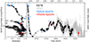 |
Fig. 1. Hardness-intensity diagram (left) and light curve (right) of the BHT Swift J1753.5–0127 during its ∼10 year-long outburst that started in 2005. The black points represent the RXTE/PCA data: the count rate is in the energy range 2 − 15 keV, while the hardness is the ratio between the rates in the 4 − 9 keV and the rates in the 2 − 4 keV energy ranges. The grey points represent the MAXI data (2 − 15 keV). The blue points indicate the five epochs of optical fast photometry considered in Veledina et al. (2017), while the red triangles indicate the two epochs of IR fast photometry reported in this work. The position of the second IR epoch in the HID and its error bars were estimated from the MAXI scaled count rate and from the ratio (not reported here) between the Swift/BAT and the MAXI scaled count rates and should only be considered as indicative of the approximate position of the source in the HID in that epoch, given the low signal-to-noise ratio of both the MAXI and BAT data. We note that the soft excursions of the source in the HID (reaching values as low as 0.3) have not been plotted for clarity of visualization (see Bu et al. 2019, for a full-scale representation of the HID). |
Infrared and X-rays observations of SWIFT J1753.5–0127
Given its long and peculiar outburst, this system has been the target of several O-IR and X-ray observations (Veledina et al. 2017, and references therein), which permitted the study of the evolution of the X-ray/optical fast variability. Such evolution was well reproduced by the aforementioned hot-inflow model, suggesting an evolution of the flow structure during the outburst (Veledina et al. 2017). In this work, we report two epochs of simultaneous X-ray/IR photometry for this source at high temporal resolution (i.e. subsecond).
2. Observations
2.1. Infrared data
We observed Swift J1753.5-0127 in the IR band for ∼10 ks using the ESO Very Large Telescope at Paranal Observatory on 15 August 2008 (ESO program 281.D-5034) and during the night between the 10 and 11 September 2012 (ESO program 089.C-0996): we refer to these dates as the first and second epoch, respectively. The data were acquired using the KS filter with the Infrared Spectrometer And Array Camera (ISAAC) (Moorwood et al. 1998) mounted on the 8.2 m UT1/Antu telescope. The detector was windowed to 256 × 256 pixels to reduce the time resolution to 62.5 ms. The data acquired by the instrument were stored in cubes, that is, groups of frames (Nframes = 995) collected consecutively over a given time interval (i.e. ∼62 s), with ∼3 s gaps in between. The weather conditions of both observations were similar, with an average seeing of around 0.7″. The absolute time accuracy is of the order of 10 milliseconds (the readout time of the detector).
The chosen 38″ × 38″ field of view contains the target, a brighter ‘reference’ star (KS = 13.19 ± 0.03), located 28.2″ south of our target (which we used to reduce the impact of atmospheric turbulence on our light curves), and two faint ‘comparison’ stars (KS = 16.12 ± 0.07 and KS = 16.68 ± 0.11) located about 15″ southwest and southeast of our target, respectively, which we used to optimise the extraction parameters. The ULTRACAM pipeline1 was used for the data reduction.
We found an average magnitude for our target during the first (second) epoch of KS = 14.95 ± 0.05 mag (15.05 ± 0.06 mag), corresponding to a flux of F = 0.70 ± 0.03 (0.64 ± 0.04) mJy. We did not correct these values for interstellar absorption.
Before performing the timing analysis, the IR light curves were barycentred to the Solar System barycentre using custom-developed MATLAB software (Ambrosino et al., in prep.). Given the relevance of this correction and the possible impact on our results of any inaccuracy, we cross-checked our barycentric correction with another software package 2 and found no significant differences.
2.2. X-ray data
We observed Swift J1753.5–0127 in the X-ray band simultaneously with the IR data in both epochs. The total exposure of the first observation obtained with the Proportional Counter Array (PCA) on board the Rossi X-ray Timing Explorer (RXTE) satellite was ∼3.5 ks (ObsIds: 93105-01-57-00, 93105-01-57-01). Spectral fitting with a simple power-law model results in a 2–10 keV unabsorbed flux of FX ∼ 10−9 ergs/s/cm2 (corresponding to a luminosity of LX ∼ 7.7 × 1036 ergs/s at 8 kpc). A light curve was extracted in the 2 − 15 keV energy range with a time resolution of 15.625 ms (1/64 s) using standard HEADAS 6.5.1 tools.
In the second epoch, the source was observed for 36 ks with the Epic-pn (PN in the following) camera on board the XMM-Newton satellite operated in TIMING mode (ObsID: 0691740201). We filtered and screened the PN data using the Science Analysis Software (SAS, Gabriel et al. 2004) v. 19.0.0 with the up-to-date calibration files. We searched for possible intervals of flaring particle background by extracting the single event (pattern = 0) high-energy (10.0–12.0 keV) light curve, but found none. We then filtered the PN data by retaining only events with pattern ≤4 (single and double pixel pattern only) and falling in the region RAWX range [30:46]. Finally, we barycentred the PN photon-arrival times using the barycen tool and adopting DE-405 Solar System ephemeris. Spectral fitting with a simple power-law model results in a 2–10 keV unabsorbed flux of FX ∼ 4 × 10⁻¹⁰ ergs/s/cm2 (corresponding to a luminosity of LX ∼ 3 × 1036 ergs/s at 8 kpc). A light curve was extracted with a time resolution of 1 ms in the 0.5 − 10 keV energy range. We verified that extracting the light curve only above 2 keV does not significantly affect the results, and therefore we decided to retain the full energy selection to optimise the throughput.
Both X-ray light curves were barycentred to the Solar System barycentre using standard HEASOFT tools. The resulting curves were then rebinned to match and align to the simultaneous IR time series. The absolute time accuracy of RXTE and XMM-Newton is 2.5 and 48 μs, respectively (Jahoda et al. 2006; Martin-Carrillo et al. 2012).
3. Analysis
3.1. Cross-correlation function
To quantify the correlation between the X-ray and IR bands, we computed the cross-correlation function (CCF) between the two time series –normalized by the product of standard deviation in each band– using the procedure described in Gandhi et al. (2010) at the maximum available time resolution of 62.5 ms. The instruments and the barycentre-correction method used for this work allow us to measure lags with a timing accuracy of a few tens of milliseconds. The two CCFs (Fig. 2) reveal a clear difference between the two epochs. The first epoch has a single peak structure that is similar to that observed in other sources (e.g. Casella et al. 2010), except for the fact that it peaks at slightly negative lags, indicating an IR lead. We quantify the position of the peak of the lag fitting a single Lorenztian function to the CCF between −2 s and 2 s, obtaining a peak lag of −0.13±0.03 s. The second CCF instead has a more complex structure: an anti-correlation dip at negative lags between about −6 s and 0 s is followed by a peak of correlation between ∼0 s and ∼10 s. Both the dip and the peak are structured in what appear to be multiple subpeaks. Closer inspection reveals that these subpeaks are consistent with being equally spaced, with a periodicity of 4 s. We tested this by fitting a sinusoidal function to the CCF, shown in Fig. 2. This is consistent with the presence in the two bands of a correlated quasi-periodic oscillation at about 0.25 Hz, which is confirmed by the power spectral analysis of the IR time series (see the following subsection). In both epochs, we assessed stationarity by dividing each exposure into two halves. The CCFs calculated independently for the two halves of each epoch do not reveal any significant difference, confirming that the time series are stationary.
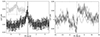 |
Fig. 2. Infrared/X-ray cross-correlation functions for the first (left) and second (right) epoch, both calculated and plotted with a 62.5 ms time resolution. Positive lags mean that IR lag X-rays. A clear correlation is detected in the first epoch, with a peak at ≈ − 0.13 s. The CCF of the second epoch shows a complex structure, with multiple anti-correlation and correlation features. As shown by the sinusoidal wave (with a period of 4 s), most of the peaks seem to be associated with the QPO at 0.25 Hz visible in the IR PDS (Fig. 3) |
3.2. Power spectral analysis
To evaluate the Fourier cross-spectral products, we followed the procedure described by Uttley et al. (2014). For both epochs, we computed the discrete Fourier transform using 512 bins per segment and a rebinning logarithmic factor of 1.2 (each bin is 20% longer than the previous one).
The X-ray and IR power density spectra (PDSs) in fractional squared root-mean-square units (Miyamoto et al. 1991) are shown in Fig. 3. Counting noise was subtracted from the X-ray PDSs but not from the IR PDSs. This is because we found a blue noise component in the PDS of both the target and comparison star, along with spurious instrumental spikes, at frequencies higher than ≈1 Hz (see Fig. A.1 and the discussion in the Appendix A). Because of this, and also owing to their low statistics, we do not model the PDSs. Nevertheless, we note that an uncorrelated noise component will not affect the measurement of the lags, only the amplitude of the CCF (or equivalently the Fourier cross-spectral coherence). We note however that the IR PDS of the second epoch (Fig. 3 top right panel) shows an excess at 0.25 Hz. This frequency is consistent with the periodicity observed in the CCF (Fig. 2, right panel). We quantify this feature by fitting it with a Lorentzian and modelling the surrounding continuum with a simple power law. We find that the QPO is significant at the ≈2.5σ level, with a fractional rms of 2.0 ± 0.4%. We note the possible presence of a modulation in the CCF that would be consistent with being associated with the QPO. We did not perform any deeper statistical analysis of the significance of this feature, as this is beyond the scope of this work.
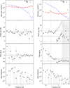 |
Fig. 3. Fourier domain analysis for the first (left) and second (right) epochs. Top Panels: X-ray (blue) and IR (red) PDS. Counting noise was subtracted from the X-ray PDSs but not from the IR, owing to the instrumental features present in the IR PDS (see Appendix A). Evidence for a quasi-periodic oscillation can be seen at ≈0.25 Hz in the PDS of the second epoch, marked by the vertical dotted line. Second Panels: Phase-lag spectrum. Positive lags mean that IR lags X-rays. While the first epoch generally has a negative lag, the second is dominated by a strong positive lag component. A clear discontinuity caused by phase wrapping is seen in the second epoch. The correction for phase wrapping is shown with grey points. The curved lines mark the estimated constant time lag (with and without phase-wrapping correction). It is apparent that at ∼2 Hz, further phase wrapping occurs, randomising the lags at higher frequencies (grey area). Third Panels: Time lags as a function of Fourier frequency. The horizontal dotted line marks the estimated constant time lag of ∼0.7 seconds between 0.4 and 2 Hz, after correcting for phase wrapping (grey points). Bottom Panels: Raw coherence as a function of the Fourier frequency. |
3.3. Cross-spectral analysis
We computed the cross-spectrum for both epochs using the recipe reported in Uttley et al. (2014), keeping the same number of segments and rebinning factor as for the PDS described in the previous section. We then extracted the time-lags, phase-lags, and raw coherence for the two epochs, shown in Fig. 3. Positive lags imply that the IR band lags the X-rays. We did not attempt to compute the intrinsic coherence owing to the presence of a blue component in the PDS, which prevents a reliable estimate of the overall noise. The strong differences observed in the CCFs of the two epochs are also reflected in the frequency domain.
During the first epoch (Fig. 3, left panel), the phase lags are negative over almost the entire frequency range, albeit with large uncertainties that make almost all data points compatible with zero lag. However, we note that the centroid and width of the CCF peak are roughly consistent with the IR lead that is observable at ν ∼ 1 Hz, as expected.
During the second epoch (Fig. 3, right panel), the phase lag spectrum instead has a different structure. The lags are nearly constant at ∼2 rad at low frequencies, up to ∼0.7 Hz where the lags change sign abruptly. Such a discontinuity suggests that the signal underwent phase wrapping. This is confirmed by shifting the phase lags above 0.7 Hz by 2π (grey points in the figure), which reveals a smooth evolution up to at least 2 Hz, where further phase wrapping probably appears and randomises the lags.
4. Discussion
We analysed two epochs of simultaneous IR and X-ray fast photometry of the black-hole transient Swift J1753.5–0127 during the late stages of its very long 2005 discovery outburst. In both epochs we detect correlated variability between the two time series, but with remarkably different properties. During the first epoch, we find that the IR variability leads the X-ray variability by ∼130 ms, as evident both in the CCF and in the frequency-dependent lags. In the second epoch, the correlation between the time series is more complex, with different lags appearing at different frequencies, suggesting the presence of multiple components.
Multiple epochs of simultaneous optical and X-ray fast photometry of Swift J1753–0127 were reported by several authors (Durant et al. 2008; Hynes et al. 2009; Durant et al. 2009, 2011), and their complex behaviour is summarised and discussed in Veledina et al. (2017) in the context of a self-consistent physical scenario with multiple components and several parameters: an expanding hot accretion flow with multiple synchrotron and Comptonization components, a variable contribution from thermal disc reprocessing and –whenever present– a contribution from a QPO. The five epochs discussed by these authors are shown in Fig. 1. In the following, we discuss possible interpretations of the newly found behaviour and test the hot-flow scenario against the new data.
4.1. First epoch
We find the IR variability to lead over the X-ray variability, and therefore we can safely rule out a jet and a reprocessing origin for the IR variable emission in this epoch, as in both cases an IR lag would be expected. Our first epoch occurred only five days after the fifth epoch considered in Veledina et al. (2017). The position of the source in the hardness-intensity diagram in the two epochs did not change significantly between the two epochs (see Fig. 1, left panel), and therefore we can safely assume the physical and geometrical conditions did not change substantially. However, the CCF found by these latter authors is very different from ours (see Fig. 4, bottom panel): they measure an anti-correlation at negative lags and a correlation at positive lags, while we observe a correlation at negative lags. Veledina et al. (2017) interpret the correlation at positive lags in terms of disc reprocessing, while the anti-correlation at negative lags is interpreted in terms of a synchrotron (optical) self-Compton (X-ray) scenario from a magnetised corona. In this scenario, the anti-correlation between synchrotron and self-Compton emission originates in fluctuations in the magnetic field causing a pivot in the spectrum around the energy that divides the two physical processes (Veledina et al. 2011). We do not observe any sign of disc reprocessing in the IR, which is perhaps not surprising given the different wavelengths (the IR-emitting region of the disc is expected to be much further away than the optical-emitting region). Also, we do not observe any of the anti-correlation predicted by the magnetised corona scenario because of the pivoting of the spectrum. However, in that scenario, another pivot is predicted (see Fig. 1 in Poutanen & Vurm 2009): below the self-absorption break, the synchrotron emission from the corona is expected to correlate with the self-Compton emission. Thus, a positive correlation between IR and X-ray emission could be expected as long as the self-absorption break is at a shorter wavelength than IR (thus λ ≲ 2 μm, as we performed our observations with the KS filter). This is in principle feasible, although it requires a surprising fine-tuning: the break must also be at a longer wavelength than optical (thus λ ≳ 0.7 μm, as the observation in the fifth optical epoch was performed with the r filter) in order to explain the anti-correlation found in Veledina et al. (2017) only five days earlier. This leaves a very narrow wavelength range. Breaks are often observed in the spectral energy distributions in the O-IR wavelength range, and existing models for the magnetised inflow do predict a break at least around those wavelengths. On the other hand, the O-IR spectral energy distribution of Swift J1753.5-0127 (or at least its non-variable component) has been well fitted by a (non-irradiated) disc thermal spectrum, with evidence for an IR excess component that takes over at longer wavelengths than the H-band (Froning et al. 2014; Wang & Wang 2014). Given the lack of perfect simultaneity between our observations and those of Veledina et al. (2017), it is difficult to draw more definite conclusions.
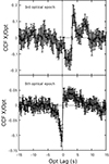 |
Fig. 4. Optical/X-ray cross-correlation functions for the third (top) and fifth (bottom) optical epoch (from Veledina et al. 2017). |
4.2. Second epoch
The CCF in our second epoch has a complex shape, which is more difficult to interpret. We observe multiple anti-correlations at negative lags and an equally structured correlation at positive lags. The CCF is somewhat similar to the CCF observed in the third and fifth optical epochs by Veledina et al. (2017) (see Fig. 4), about seven and four years earlier, respectively. Both CCFs were modelled by Veledina et al. (2017) in the context of the expanding hot flow model described above. Thus, it is natural to expect that the same model might succeed in describing our CCF. However, some of the complex structures we observe are most probably caused by the presence of a QPO (Fig. 2), which was not present in the fifth optical epoch. A QPO at a very similar frequency was instead present in the third epoch and apparent in the CCF, which is surprisingly similar in appearance to the one we measured in our second epoch, albeit shifted by 2 seconds towards positive (optical) lags. As a result of these and further differences (including the X-ray brightness), the two epochs were modelled with two rather different sets of parameters. The phase lags of those two epochs are completely different from each other, demonstrating that the CCFs alone are not always sufficiently informative. A QPO at lower frequencies was present in the fourth optical epoch, and apparent in the CCF (Veledina et al. 2015).
Given the limitation of the technique and the complexity of our CCF, cross-spectral analysis here can help us separate different components at different timescales, revealing the possible roles of the alternative processes. Looking at Fig. 3, we can identify two different behaviours or regimes in the lags: at low frequencies, the phase lags are consistent with being constant at around ∼2 radians, corresponding to a lag of a few seconds, which decreases with frequency. The amplitude of these lags and the frequency intervals in which they appear suggest they could be consistent with the model proposed by Veledina et al. (2017). At high frequencies, on the other hand, above ∼0.4 Hz, the phase lags increase with frequency, corresponding to a constant lag at ∼0.7 s. By integrating the phase lag between 0.4 and 0.9 Hz (i.e. where the phase-wrapping effect is still not dominant) we obtain an IR lag of 0.72 ± 0.16s. A constant lag at these frequencies –albeit at a shorter value of the order of 0.1 s– has been observed in other BHTs and associated with the jet (see the following subsection). For frequencies above ∼2 Hz, there is evidence for intense phase wrapping, which makes it impossible to extract useful information. No clear feature can be seen in the lags at the frequency of the QPO (≃0.25 Hz) owing to the low significance of the QPO in the PDSs. For the same reason, we cannot quantify the QPO lag from the modulation apparent in the CCF, considering also the complexity of the CCF itself. We note however that, qualitatively, the modulation in the CCF suggests that the lag is small, perhaps consistent with the zero QPO lag measured by Veledina et al. (2015) in the optical band.
4.3. A jet in a radio-quiet source?
The most evident property of the correlated variability in Swift J1753.5–0127 is its complex evolution. Only two of the five epochs of X-ray/optical variability reported by Durant et al. (2008), Hynes et al. (2009), Durant et al. (2009), and Durant et al. (2011), and discussed by Veledina et al. (2017), are similar to each other, while the others show remarkably different features. This complexity is confirmed by our results. Not only do our two epochs of X-ray/IR variability differ enormously from each other, but they are also rather different from all the optical epochs, even when they are very close in time. Even when the CCFs show some similarities, the time lags reveal important differences.
While there is no evidence of any jet contribution to the IR emission in our first epoch, our second epoch shows time lags somewhat similar to those observed in other BHTs, where they were interpreted as a jet signature. If we compare the time lags from our second epoch (Fig. 5) with those reported for GX 339–4 in Gandhi et al. (2010, Fig. 18) and Vincentelli et al. (2019, Fig. 2), for V404 Cyg in Gandhi et al. (2017, Fig. S2), and for MAXI J1820+070 in Paice et al. (2019, Fig. 2), the similarities are striking. In all cases, a clear component with a constant lag at ∼0.1 − 0.2 seconds can be identified at frequencies around 1 Hz. This component has been associated –very securely in some cases, and by analogy in others– with a compact jet. Thus, it is natural to consider the possibility that we have also detected variable jet emission in Swift J1753.5–0127. If this is the case, questions remain as to why we measured lag 0.7 s instead of the ‘usual’ 0.1–0.2 s, and why no jet contribution is detected in our first epoch, despite the very similar X-ray hardness. We note that the X-ray luminosity during our second epoch was very similar to (a factor of ∼2 brighter than) the X-ray luminosity at which the 0.1 s lag was measured in GX 339-4 (Casella et al. 2010).
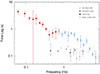 |
Fig. 5. X-ray/IR time lags for Epoch 2. The red-filled points are the original data points, while the empty blue circles are the time lags computed assuming a 2π shift, i.e. after taking into account the phase wrapping effect. Two components are evident, with a transition at around 0.4 Hz. In dark grey, we report previous measurements of a constant time lag at frequencies around 1 Hz (see text). |
The longer jet lag in Swift J1753.5–0127 might be related to the well-known peculiar properties of the jet in this source, which is one of the so-called radio-quiet BHTs (Soleri & Fender 2011; Gallo et al. 2012; Espinasse & Fender 2018; Motta et al. 2018). This definition comes from the behaviour of this source in the radio/X-ray plane, where it lies below the ‘standard’ track (Soleri et al. 2010), and suggests that the jets in these sources have different radiative properties, and are perhaps weaker than in ‘standard’ sources. Thus, it would not be too surprising if the jet in Swift J1753.5–0127 were also found to have different variability properties. This could be somewhat confirmed by the fact that, in at least one case, the jet break in Swift J1753.5-0127 has been constrained to be at frequencies lower than 3.6 × 10¹² Hz (Tomsick et al. 2015), at least an order of magnitude lower than in GX 339-4 (Gandhi et al. 2011) and in several other BHTs (Russell et al. 2013). The differences between the two epochs could be due to two different factors: On the one hand, the second epoch has a lower count rate than the first epoch. The jet could have appeared as the source was heading towards quiescence, while it was not present years earlier in a brighter state. Several radio-quiet BHTs have shown a transition back from the radio-quiet branch to the standard branch in the radio/X-ray plane when heading towards quiescence (e.g. Coriat et al. 2011), suggesting that the jet becomes stronger at low accretion rates. Evidence for this happening also in Swift J1753.5–0127 was reported (Kolehmainen et al. 2016). On the other hand, the X-ray variability in the two epochs differs substantially (Fig. 6), with a clear change in the slope of the power spectrum below the high-frequency break. The two shapes are consistent with the typical PDS observed in the hard states (Belloni et al. 2005). A link between the shape of the X-ray PDS and the radio properties has recently been suggested for GRS 1915+105 (Méndez et al. 2022) and GX 339-4 (Zhang et al. 2024). In the context of the jet internal-shock model (Malzac et al. 2018), such a difference in the slope of the PDS has been shown to correspond to different jet spectral properties in the two epochs, with the self-absorption break shifting by as much as four orders of magnitude in wavelength (Malzac 2014). Thus, again it would not be too surprising to find that, in the second epoch, the jet is much brighter in the IR than in the first epoch. This could in principle also be related to a variable jet speed with luminosity, as suggested by Russell et al. (2015) to explain the peculiar behaviour in the radio/X-ray plane of MAXI J1836-194 (although this system most probably has a lower inclination than Swift J1753.5-0127). As the IR flux was similar in the two epochs, a different jet brightness in the IR would also imply a variable contribution from a different component.
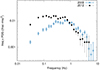 |
Fig. 6. Comparison between the X-ray PDSs measured during our 2008 and 2012 observations. A clear change of the slope is observed below the high-frequency break. |
5. Conclusions
We observed a complex behaviour in the correlated IR/X-ray fast variability of the BHT Swift J1753.5-0127 during its ten-year 2005 discovery outburst. In the first of our two epochs, the data can be interpreted in terms of synchrotron-self-Compton emission from a magnetised hot flow. In the second epoch, the data reveal a more complex context. The low-frequency behaviour is consistent with a combination of disc reprocessing and a magnetised hot flow. However, the constant lags at ∼0.7 s at high frequencies are reminiscent of the constant lags observed in a similar frequency range at ∼0.1 s in other sources. These constant lags are usually considered a signature of O-IR synchrotron emission from a compact jet lagging behind the X-ray emission from the inflow by 0.1 seconds, which suggests a similar interpretation for SWIFT J1753.5-0127. The longer lag we measure could be due to the different radiative properties of the jet in this source. The complexity of the behaviour, the lack of broader multi-wavelength data, and the overall paucity of datasets make these interpretations only tentative. These results underline the need for denser campaigns of strictly simultaneous multi-wavelength fast photometry to reach a broader and deeper understanding of the complex variable spectral properties of black-hole transients.
Acknowledgments
Based on observations collected at the European Southern Observatory under ESO programmes 281.D-5034 and 089.C-0996. PC, FMV and all the Authors acknowledge the long-term contribution of Tomaso Belloni to this project. Tomaso sadly passed away in August 2023 and will be sorely missed. The Authors thank the Team Meeting at the International Space Science Institute (Bern) for fruitful discussions and were supported by the ISSI International Team project #440. FMV acknowledges support from the grant FJC2020-043334-I financed by MCIN/AEI/10.13039/501100011033 and Next Generation EU/PRTR, as well as from the grant PID2020-114822GB-I00. PC acknowledges financial support from the Italian Space Agency and National Institute for Astrophysics, ASI/INAF, under agreement ASI-INAF n.2017-14-H.0. AV acknowledges support from the Research Council of Finland grant 355672. Nordita is supported in part by NordForsk. MI is supported by the AASS Ph.D. joint research programme between the University of Rome “Sapienza” and the University of Rome “Tor Vergata”, with the collaboration of the National Institute of Astrophysics (INAF). The ISAAC data are available from the ESO Data Archive (https://archive.eso.org/eso/eso_archive_main.html). The RXTE data are available from the HEASARC Data Archive (https://heasarc.gsfc.nasa.gov/docs/archive.html). The XMM-Newton data are available from the XMM-Newton Science Archive (https://nxsa.esac.esa.int/nxsa-web/). The MAXI data used in Fig.1 are available from the MAXI website (http://maxi.riken.jp/top/index.html). The BAT data used to estimate the hardness of the source during the second epoch are available from the Neil Gehrels Swift Observatory archive (https://swift.gsfc.nasa.gov/results/transients/).
References
- Alabarta, K., Altamirano, D., Méndez, M., et al. 2021, MNRAS, 507, 5507 [NASA ADS] [CrossRef] [Google Scholar]
- Bambi, C., Brenneman, L. W., Dauser, T., et al. 2021, Space Sci. Rev., 217, 65 [CrossRef] [Google Scholar]
- Belloni, T. M., & Stella, L. 2014, Space Sci. Rev., 183, 43 [NASA ADS] [CrossRef] [Google Scholar]
- Belloni, T., Homan, J., Casella, P., et al. 2005, A&A, 440, 207 [NASA ADS] [CrossRef] [EDP Sciences] [Google Scholar]
- Belloni, T. M., Motta, S. E., & Muñoz-Darias, T. 2011, Bull. Astron. Soc. India, 39, 409 [Google Scholar]
- Blandford, R. D., & Königl, A. 1979, ApJ, 232, 34 [Google Scholar]
- Brocksopp, C., Bandyopadhyay, R. M., & Fender, R. P. 2004, New Astron., 9, 249 [CrossRef] [Google Scholar]
- Bu, Q., Tao, L., Lu, Y., et al. 2019, MNRAS, 487, 1439 [NASA ADS] [CrossRef] [Google Scholar]
- Casella, P., & Pe’er, A. 2009, ApJ, 703, L63 [Google Scholar]
- Casella, P., Belloni, T., & Stella, L. 2005, ApJ, 629, 403 [Google Scholar]
- Casella, P., Maccarone, T. J., O’Brien, K., et al. 2010, MNRAS, 404, L21 [NASA ADS] [Google Scholar]
- Corbel, S., & Fender, R. P. 2002, ApJ, 573, L35 [NASA ADS] [CrossRef] [Google Scholar]
- Corbel, S., Aussel, H., Broderick, J. W., et al. 2013, MNRAS, 431, L107 [NASA ADS] [CrossRef] [Google Scholar]
- Coriat, M., Corbel, S., Prat, L., et al. 2011, MNRAS, 414, 677 [Google Scholar]
- Corral-Santana, J. M., Casares, J., Muñoz-Darias, T., et al. 2016, A&A, 587, A61 [NASA ADS] [CrossRef] [EDP Sciences] [Google Scholar]
- Debnath, D., Jana, A., Chakrabarti, S. K., Chatterjee, D., & Mondal, S. 2017, ApJ, 850, 92 [NASA ADS] [CrossRef] [Google Scholar]
- Done, C., Gierliński, M., & Kubota, A. 2007, A&ARv, 15, 1 [Google Scholar]
- Drappeau, S., Malzac, J., Coriat, M., et al. 2017, MNRAS, 466, 4272 [NASA ADS] [Google Scholar]
- Durant, M., Gandhi, P., Shahbaz, T., et al. 2008, ApJ, 682, L45 [NASA ADS] [CrossRef] [Google Scholar]
- Durant, M., Gandhi, P., Shahbaz, T., Peralta, H. H., & Dhillon, V. S. 2009, MNRAS, 392, 309 [NASA ADS] [CrossRef] [Google Scholar]
- Durant, M., Shahbaz, T., Gandhi, P., et al. 2011, MNRAS, 410, 2329 [NASA ADS] [CrossRef] [Google Scholar]
- Esin, A. A., McClintock, J. E., & Narayan, R. 1997, ApJ, 489, 865 [NASA ADS] [CrossRef] [Google Scholar]
- Espinasse, M., & Fender, R. 2018, MNRAS, 473, 4122 [Google Scholar]
- Fender, R. P. 2001, MNRAS, 322, 31 [NASA ADS] [CrossRef] [Google Scholar]
- Fender, R. P., Homan, J., & Belloni, T. M. 2009, MNRAS, 396, 1370 [NASA ADS] [CrossRef] [Google Scholar]
- Froning, C. S., Maccarone, T. J., France, K., et al. 2014, ApJ, 780, 48 [Google Scholar]
- Gabriel, C., Denby, M., Fyfe, D. J., et al. 2004, ASP Conf. Ser., 314, 759 [Google Scholar]
- Gallo, E., Miller, B. P., & Fender, R. 2012, MNRAS, 423, 590 [Google Scholar]
- Gandhi, P., Dhillon, V. S., Durant, M., et al. 2010, MNRAS, 407, 2166 [NASA ADS] [CrossRef] [Google Scholar]
- Gandhi, P., Blain, A. W., Russell, D. M., et al. 2011, ApJ, 740, L13 [NASA ADS] [CrossRef] [Google Scholar]
- Gandhi, P., Bachetti, M., Dhillon, V. S., et al. 2017, Nat. Astron., 1, 859 [NASA ADS] [CrossRef] [Google Scholar]
- Gilfanov, M. 2009, Lecture Notes Phys., 794, 17 [NASA ADS] [CrossRef] [Google Scholar]
- Hjellming, R. M., & Johnston, K. J. 1988, ApJ, 328, 600 [NASA ADS] [CrossRef] [Google Scholar]
- Hynes, R. I., Brien, K. O., Mullally, F., & Ashcraft, T. 2009, MNRAS, 399, 281 [CrossRef] [Google Scholar]
- Ingram, A. R., & Motta, S. E. 2019, New Astron. Rev., 85, 101524 [Google Scholar]
- Jahoda, K., Markwardt, C. B., Radeva, Y., et al. 2006, ApJS, 163, 401 [NASA ADS] [CrossRef] [Google Scholar]
- Kalamkar, M., Casella, P., Uttley, P., et al. 2016, MNRAS, 460, 3284 [NASA ADS] [CrossRef] [Google Scholar]
- Kanbach, G., Straubmeier, C., Spruit, H. C., & Belloni, T. 2001, Nature, 414, 180 [NASA ADS] [CrossRef] [Google Scholar]
- Kolehmainen, M., Fender, R., Jonker, P. G., et al. 2016, Astron. Nachr., 337, 485 [NASA ADS] [CrossRef] [Google Scholar]
- Koljonen, K. I. I., Maccarone, T., McCollough, M. L., et al. 2018, A&A, 612, A27 [NASA ADS] [CrossRef] [EDP Sciences] [Google Scholar]
- Maccarone, T. J., Osler, A., Miller-Jones, J. C. A., et al. 2020, MNRAS, 498, L40 [NASA ADS] [CrossRef] [Google Scholar]
- Malzac, J. 2014, MNRAS, 443, 299 [NASA ADS] [CrossRef] [Google Scholar]
- Malzac, J., Merloni, A., & Fabian, A. C. 2004, MNRAS, 351, 253 [NASA ADS] [CrossRef] [Google Scholar]
- Malzac, J., Kalamkar, M., Vincentelli, F., et al. 2018, MNRAS, 480, 2054 [NASA ADS] [CrossRef] [Google Scholar]
- Martin-Carrillo, A., Kirsch, M. G. F., Caballero, I., et al. 2012, A&A, 545, A126 [NASA ADS] [CrossRef] [EDP Sciences] [Google Scholar]
- Méndez, M., Karpouzas, K., García, F., et al. 2022, Nat. Astron., 6, 577 [CrossRef] [Google Scholar]
- Merloni, A., Di Matteo, T., & Fabian, A. C. 2000, MNRAS, 318, L15 [NASA ADS] [CrossRef] [Google Scholar]
- Miyamoto, S., Kimura, K., Kitamoto, S., Dotani, T., & Ebisawa, K. 1991, ApJ, 383, 784 [NASA ADS] [CrossRef] [Google Scholar]
- Moorwood, A., Cuby, J. G., Biereichel, P., et al. 1998, Messenger, 94, 7 [Google Scholar]
- Motch, C., Ilovaisky, S. A., & Chevalier, C. 1982, A&A, 109, L1 [Google Scholar]
- Motch, C., Ricketts, M. J., Page, C. G., Ilovaisky, S. A., & Chevalier, C. 1983, A&A, 119, 171 [Google Scholar]
- Motta, S. E., Casella, P., Henze, M., et al. 2015, MNRAS, 447, 2059 [NASA ADS] [CrossRef] [Google Scholar]
- Motta, S. E., Casella, P., & Fender, R. P. 2018, MNRAS, 478, 5159 [Google Scholar]
- Paice, J. A., Gandhi, P., Shahbaz, T., et al. 2019, MNRAS, 490, L62 [NASA ADS] [CrossRef] [Google Scholar]
- Paice, J. A., Gandhi, P., Shahbaz, T., et al. 2021, MNRAS, 505, 3452 [NASA ADS] [CrossRef] [Google Scholar]
- Plotkin, R. M., Bright, J., Miller-Jones, J. C. A., et al. 2017, ApJ, 848, 92 [NASA ADS] [CrossRef] [Google Scholar]
- Poutanen, J., & Veledina, A. 2014, Space Sci. Rev., 183, 61 [CrossRef] [Google Scholar]
- Poutanen, J., & Vurm, I. 2009, ApJ, 690, L97 [NASA ADS] [CrossRef] [Google Scholar]
- Poutanen, J., Krolik, J. H., & Ryde, F. 1997, MNRAS, 292, L21 [NASA ADS] [Google Scholar]
- Poutanen, J., Veledina, A., & Zdziarski, A. A. 2018, A&A, 614, A79 [NASA ADS] [CrossRef] [EDP Sciences] [Google Scholar]
- Remillard, R. A., & McClintock, J. E. 2006, ARA&A, 44, 49 [Google Scholar]
- Russell, D. M., Markoff, S., Casella, P., et al. 2013, MNRAS, 429, 815 [NASA ADS] [CrossRef] [Google Scholar]
- Russell, T. D., Miller-Jones, J. C. A., Curran, P. A., et al. 2015, MNRAS, 450, 1745 [Google Scholar]
- Shakura, N. I., & Sunyaev, R. A. 1973, A&A, 500, 33 [NASA ADS] [Google Scholar]
- Shaw, A. W., Gandhi, P., Altamirano, D., et al. 2016, MNRAS, 458, 1636 [NASA ADS] [CrossRef] [Google Scholar]
- Soleri, P., & Fender, R. 2011, MNRAS, 413, 2269 [Google Scholar]
- Soleri, P., Fender, R., Tudose, V., et al. 2010, MNRAS, 406, 1471 [NASA ADS] [Google Scholar]
- Soleri, P., Muñoz-Darias, T., Motta, S., et al. 2013, MNRAS, 429, 1244 [NASA ADS] [CrossRef] [Google Scholar]
- Tetarenko, B. E., Sivakoff, G. R., Heinke, C. O., & Gladstone, J. C. 2016, ApJS, 222, 15 [Google Scholar]
- Tetarenko, A. J., Casella, P., Miller-Jones, J. C. A., et al. 2021, MNRAS, 504, 3862 [NASA ADS] [CrossRef] [Google Scholar]
- Tomsick, J. A., Rahoui, F., Kolehmainen, M., et al. 2015, ApJ, 808, 85 [NASA ADS] [CrossRef] [Google Scholar]
- Uttley, P., Cackett, E. M., Fabian, A. C., Kara, E., & Wilkins, D. R. 2014, A&ARv., 22, 72 [NASA ADS] [CrossRef] [Google Scholar]
- Veledina, A., Poutanen, J., & Vurm, I. 2011, ApJ, 737, L17 [NASA ADS] [CrossRef] [Google Scholar]
- Veledina, A., Revnivtsev, M. G., Durant, M., Gandhi, P., & Poutanen, J. 2015, MNRAS, 454, 2855 [NASA ADS] [CrossRef] [Google Scholar]
- Veledina, A., Gandhi, P., Hynes, R., et al. 2017, MNRAS, 470, 48 [CrossRef] [Google Scholar]
- Vincentelli, F. M., Casella, P., Maccarone, T. J., et al. 2018, MNRAS, 477, 4524 [NASA ADS] [CrossRef] [Google Scholar]
- Vincentelli, F. M., Casella, P., Petrucci, P., et al. 2019, ApJ, 887, L19 [NASA ADS] [CrossRef] [Google Scholar]
- Vincentelli, F. M., Casella, P., Russell, D. M., et al. 2021, MNRAS, 503, 614 [NASA ADS] [CrossRef] [Google Scholar]
- Wang, X., & Wang, Z. 2014, ApJ, 788, 184 [NASA ADS] [CrossRef] [Google Scholar]
- Zdziarski, A. A., & Gierliński, M. 2004, Prog. Theor. Phys. Suppl., 155, 99 [CrossRef] [Google Scholar]
- Zhang, Y., Méndez, M., Motta, S. E., et al. 2024, MNRAS, 527, 5638 [Google Scholar]
- Zurita, C., Durant, M., Torres, M. A. P., et al. 2008, ApJ, 681, 1458 [NASA ADS] [CrossRef] [Google Scholar]
Appendix A: Comparison star’s power spectrum
To understand the nature of the blue noise present in the IR power spectrum of our target, we also checked the power spectrum obtained from the comparison star. The results for both epochs are shown in Fig. A.1. It is clear that in both cases there is a source of blue noise which starts dominating above a few Hz. We also notice the presence of spurious peaks at around 4 and 6 Hz (somewhat visible also in the target PDSs in Fig.3, top panels). Similar features had already been detected in ISAAC data (Casella et al. 2010; Vincentelli et al. 2018). These peaks are clearly instrumental, while the blue noise is most probably caused by readout noise. No additional feature is observed at lower frequencies, indicating that power measurements below ∼ 1 Hz are safe.
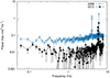 |
Fig. A.1. Infrared power spectral density of the brighter comparison star during the two epochs of observation. |
All Tables
All Figures
|
Fig. 1. Hardness-intensity diagram (left) and light curve (right) of the BHT Swift J1753.5–0127 during its ∼10 year-long outburst that started in 2005. The black points represent the RXTE/PCA data: the count rate is in the energy range 2 − 15 keV, while the hardness is the ratio between the rates in the 4 − 9 keV and the rates in the 2 − 4 keV energy ranges. The grey points represent the MAXI data (2 − 15 keV). The blue points indicate the five epochs of optical fast photometry considered in Veledina et al. (2017), while the red triangles indicate the two epochs of IR fast photometry reported in this work. The position of the second IR epoch in the HID and its error bars were estimated from the MAXI scaled count rate and from the ratio (not reported here) between the Swift/BAT and the MAXI scaled count rates and should only be considered as indicative of the approximate position of the source in the HID in that epoch, given the low signal-to-noise ratio of both the MAXI and BAT data. We note that the soft excursions of the source in the HID (reaching values as low as 0.3) have not been plotted for clarity of visualization (see Bu et al. 2019, for a full-scale representation of the HID). |
| In the text | |
|
Fig. 2. Infrared/X-ray cross-correlation functions for the first (left) and second (right) epoch, both calculated and plotted with a 62.5 ms time resolution. Positive lags mean that IR lag X-rays. A clear correlation is detected in the first epoch, with a peak at ≈ − 0.13 s. The CCF of the second epoch shows a complex structure, with multiple anti-correlation and correlation features. As shown by the sinusoidal wave (with a period of 4 s), most of the peaks seem to be associated with the QPO at 0.25 Hz visible in the IR PDS (Fig. 3) |
| In the text | |
|
Fig. 3. Fourier domain analysis for the first (left) and second (right) epochs. Top Panels: X-ray (blue) and IR (red) PDS. Counting noise was subtracted from the X-ray PDSs but not from the IR, owing to the instrumental features present in the IR PDS (see Appendix A). Evidence for a quasi-periodic oscillation can be seen at ≈0.25 Hz in the PDS of the second epoch, marked by the vertical dotted line. Second Panels: Phase-lag spectrum. Positive lags mean that IR lags X-rays. While the first epoch generally has a negative lag, the second is dominated by a strong positive lag component. A clear discontinuity caused by phase wrapping is seen in the second epoch. The correction for phase wrapping is shown with grey points. The curved lines mark the estimated constant time lag (with and without phase-wrapping correction). It is apparent that at ∼2 Hz, further phase wrapping occurs, randomising the lags at higher frequencies (grey area). Third Panels: Time lags as a function of Fourier frequency. The horizontal dotted line marks the estimated constant time lag of ∼0.7 seconds between 0.4 and 2 Hz, after correcting for phase wrapping (grey points). Bottom Panels: Raw coherence as a function of the Fourier frequency. |
| In the text | |
|
Fig. 4. Optical/X-ray cross-correlation functions for the third (top) and fifth (bottom) optical epoch (from Veledina et al. 2017). |
| In the text | |
|
Fig. 5. X-ray/IR time lags for Epoch 2. The red-filled points are the original data points, while the empty blue circles are the time lags computed assuming a 2π shift, i.e. after taking into account the phase wrapping effect. Two components are evident, with a transition at around 0.4 Hz. In dark grey, we report previous measurements of a constant time lag at frequencies around 1 Hz (see text). |
| In the text | |
|
Fig. 6. Comparison between the X-ray PDSs measured during our 2008 and 2012 observations. A clear change of the slope is observed below the high-frequency break. |
| In the text | |
|
Fig. A.1. Infrared power spectral density of the brighter comparison star during the two epochs of observation. |
| In the text | |
Current usage metrics show cumulative count of Article Views (full-text article views including HTML views, PDF and ePub downloads, according to the available data) and Abstracts Views on Vision4Press platform.
Data correspond to usage on the plateform after 2015. The current usage metrics is available 48-96 hours after online publication and is updated daily on week days.
Initial download of the metrics may take a while.