| Issue |
A&A
Volume 689, September 2024
|
|
|---|---|---|
| Article Number | A299 | |
| Number of page(s) | 18 | |
| Section | Numerical methods and codes | |
| DOI | https://doi.org/10.1051/0004-6361/202450437 | |
| Published online | 20 September 2024 | |
Prospects of directly using closure traces for imaging in very long baseline interferometry
1
Max-Planck-Institut für Radioastronomie, Auf dem Hügel 69, 53121 Bonn (Endenich), Germany
2
Jansky Fellow of National Radio Astronomy Observatory, 1011 Lopezville Rd, Socorro, NM 87801, USA
Received:
18
April
2024
Accepted:
29
July
2024
Abstract
Context. The reconstruction of the polarization of a source in radio interferometry is a challenging calibration problem since the reconstruction strongly depends on the gains and leakages, which need to be inferred along with the image. This is particularly true for the Event Horizon Telescope (EHT) due to its small number of antennas, low signal-to-noise ratio, and large gain corruptions.
Aims. To recover linear polarization, one has to either infer the leakages and gains together with the image structure or rely completely on calibration-independent closure quantities. While the first approach has been explored in very long baseline interferometry (VLBI) for a long time, the latter has been less studied for polarimetry.
Methods. Closure traces are a recently proposed concept of closure quantities that, in contrast to closure phases and closure amplitudes, are independent of both gains and leakages and carry the relevant information about the polarization of the source. Here we explore how closure traces can be directly fitted to create an image, and we identify an imaging pipeline that succeeds in direct imaging from closure traces.
Results. Since closure traces have a number of inherent degeneracies, multiple local image modes that can fit the data are detected. Therefore, a multi-objective imaging technique is needed to correctly sample this multi-modality.
Conclusions. Closure traces are not constraining enough for the current EHT configuration to recover an image directly, mainly due to the small number of antennas. For planned successors of the EHT, however (with a significantly larger number of antennas), this option will become feasible and will be competitive with techniques that use imaging with residual leakages.
Key words: methods: numerical / techniques: high angular resolution / techniques: image processing / techniques: interferometric / galaxies: jets
Corresponding author; This email address is being protected from spambots. You need JavaScript enabled to view it.
© The Authors 2024
 Open Access article, published by EDP Sciences, under the terms of the Creative Commons Attribution License (https://creativecommons.org/licenses/by/4.0), which permits unrestricted use, distribution, and reproduction in any medium, provided the original work is properly cited.
This article is published in open access under the Subscribe to Open model.
Open Access funding provided by Max Planck Society.
1 Introduction
In very long baseline interferometry (VLBI), multiple antennas are combined into a single array. The correlated signal of an antenna pair gives rise to the Fourier transform of the true sky brightness distribution (visibilities), with the spatial frequency defined by the baseline separating the two antennas projected on the sky plane, as described by the Cittert-Zernike theorem (Thompson et al. 2017). Imaging these data is an ill-posed inverse problem due to the sparsity of the coverage of measured Fourier coefficients (uv coverage). Additionally, we have to deal with instrumental noise and direction-independent, station-based antenna calibration effects at the imaging stage. This makes the imaging problem challenging, particularly with the low phase stability encountered when observing at high frequencies and in very sparse settings.
VLBI observations in polarimetric light are particularly interesting for the study of active galactic nucleus (AGN) jets since synchrotron radiation is expected to be polarized. In fact, polarimetric studies of AGNs play a vital role in the understanding of the magnetic field in AGNs (e.g., Homan et al. 2011; Gabuzda 2021; Pötzl et al. 2021; Kramer & MacDonald 2021; Event Horizon Telescope Collaboration 2021a; Event Horizon Telescope Collaboration 2021b; Ricci et al. 2022; Kramer et al. 2024). However, polarimetric studies pose additional calibration challenges. Most importantly, we have to correct the measurements for leakage terms between orthogonal polarization feeds. These can be measured with observations of the calibrator source, which appears ideally as a point source. However, when the calibrator source has poor parallactic coverage, or is resolved on its own as is common in millimeter VLBI experiments, the leakage estimation is more challenging.
Historically, the imaging and calibration problem was solved via a hybrid inverse modeling approach (Pearson & Readhead 1984). Data are imaged in total intensity and then self-calibrated, alternating between these two procedures. This imaging can be done using the CLEAN algorithm (Högbom 1974) or some of its successors (Clark 1980; Schwab 1984; Bhatnagar & Cornwell 2004; Cornwell 2008; Rau & Cornwell 2011; Offringa & Smirnov 2017; Müller & Lobanov 2023b). CLEAN is a greedy matching pursuit algorithm that models the image as a set of delta components in user-defined search windows. Self-calibration is the procedure of identifying the station-based gains that optimize the match between the model visibilities and the observed visibilities. In this sense, hybrid imaging can be understood as a two-step optimization procedure. Typically, the dataset is imaged and self-calibrated in total intensity, the leakage terms are then calibrated, and the imaging procedure is repeated for all four Stokes parameters (Cotton 1993; Park et al. 2021; Martí-Vidal et al. 2021).
CLEAN is the de facto standard in VLBI. However, CLEAN has well-known limitations (e.g., see the discussions in Müller & Lobanov 2023b; Pashchenko et al. 2023) that are most pronounced in sparse settings (for example, see the performance comparisons in Event Horizon Telescope Collaboration 2019a; Arras et al. 2019; Müller & Lobanov 2022, 2023b; Müller et al. 2024; Roelofs et al. 2023a).
Recently, forward modeling approaches have been proposed for sparse VLBI imaging in the framework of regularized maximum likelihood (RML) methods (see Honma et al. 2014; Akiyama et al. 2017b,a; Chael et al. 2016, 2018, 2023), compressive sensing (Müller & Lobanov 2022, 2023a), Bayesian imaging (Broderick et al. 2020b; Arras et al. 2022; Tiede 2022), and multi-objective evolution (Müller et al. 2023; Mus et al. 2024b,a). These reconstruction algorithms perform better than CLEAN in terms of resolution, dynamic range, and accuracy in an Event Horizon Telescope-like setting.
Several strategies can be used adapt the self-calibration and leakage calibration in these forward modeling frameworks. They can be broadly divided into two opposite philosophies. First, we can add the unknown gains and leakage terms to the vector of unknowns and infer them during the imaging (Kim et al. 2024) or alternate it with the imaging (e.g., with the strategy for time-dynamic and polarimetric reconstructions applied by Mus et al. 2024b). Second, we can directly fit data products that are robust against gains and/or leakages and subsequently ignore them in the rest of the procedure. This was done using closure-only imaging in various imaging frameworks (Chael et al. 2018; Müller & Lobanov 2022; Müller et al. 2023) that utilize closure phases and closure amplitudes. Moreover, calibration-robust polarization fractions were proposed for the reconstruction of the polarimet-ric signal for sparse millimeter VLBI (Johnson et al. 2017; Event Horizon Telescope Collaboration 2021a; Roelofs et al. 2023b). Blackburn et al. (2020) has demonstrated that the direct fitting of robust, self-calibration data products such as closures is the equivalent to a Bayesian marginalization over completely unknown gains, for example with flat priors. Bayesian methods would only show an improvement if informative priors are incorporated into these nuisance parameters. This mathematical equivalence is not necessarily true for RML approaches since the regularizers do not in all cases have a Bayesian interpretation, and overall the relative balancing between the data fidelity term and the regularization terms may be affected. Moreover, even for full Bayesian algorithms, this equivalence may not always been achieved in numerical practice since marginalization over the gains and leakages may include integrating potentially high-dimensional multimodal posterior distributions, which are only known approximately.
Closure traces are a novel concept of closure quantities introduced by Broderick et al. (2020a). They are constructed from a quadrangle of antennas via a combination of Stokes matrices. They are in particular independent of most types of data corruption, for example gains, antenna feed rotation, and leakage terms. Moreover, they contain closure phases and closure amplitudes as special cases in the unpolarized limit. A variant defined on triangles has been proposed by Samuel et al. (2022), based on a full gauge theory for closure products (Thyagarajan et al. 2022; Thyagarajan & Carilli 2022). It is natural to attempt to directly fit closure traces to infer the polarimetric features of a source. The use of closure traces for the polarimetric calibration may be imperative in all situations in which the parallactic angle coverage of the calibrator is insufficient for a proper calibration. A first pioneering work in this direction was carried out by Albentosa-Ruiz & Marti-Vidal (2023), although in a model-fitting rather than an imaging framework. In this manuscript we study the prospects of constructing an imaging algorithm that, for the first time, fits directly to the closure traces rather than the visibilities.
Such an imaging application has the specific advantage of being calibration-independent, thus avoiding the self-referencing, and necessarily local, hybrid imaging approach. However, closure traces are nontrivial complex quantities that are constructed out of the observables in an interferometric experiment (i.e., visibilities), and consequently the number of statistically independent closure traces is smaller than the number of independent visibilities. Roughly speaking, by constructing data products that are independent of the gains and leakages, we depend on less constraining data products, a fact that manifests in a number of degeneracies, as listed by Broderick et al. (2020a). To account for these degeneracies and the increased sparsity during the imaging, we have to account for the missing information and non-convex optimization landscape by using stricter regular-ization information. One such approach, namely multi-objective optimization (Müller et al. 2023; Mus et al. 2024a), is presented in this manuscript.
For this work we focused on two cases. First we studied VLBI, specifically the Event Horizon Telescope (EHT) and its planned successors. This data regime stands out as a particularly interesting area of application of calibration-independent imaging since the high frequency, global baselines, and sparsity of the array render the initial calibration (especially with respect to phases) very challenging (Janssen et al. 2022), and the imaging and self-calibration may be at risk of falling into local extrema and method-specific biases.
Second, we studied the application of closure trace imaging in denser radio interferometers, in this case the Atacama Large Millimeter Array (ALMA), and we reproduced the experiment performed by Albentosa-Ruiz & Marti-Vidal (2023). While the Event Horizon Telescope Collaboration has contributed a wide variety of imaging and calibration tools (including the forward modeling techniques and closure quantities studied in this manuscript), and continues to be the target of active and ongoing developments, a transfer of these ideas to general inter-ferometric imaging has only been done on a few occasions (e.g., recently by Albentosa-Ruiz & Marti-Vidal 2023; Fuentes et al. 2023; Lu et al. 2023; Kramer et al. 2024; Müller et al. 2024). By testing closure trace imaging with a real ALMA observation, we also aim to contribute to the transfer of knowledge and methodologies gained using the EHTC to general interferometric experiments.
In the pursuit of these efforts toward direct imaging from closure traces, both RML (Honma et al. 2014; Chael et al. 2016, 2018, 2023; Akiyama et al. 2017b,a; Müller & Lobanov 2022, 2023a; Müller et al. 2023; Mus et al. 2024a) and Bayesian approaches (Broderick et al. 2020b; Pesce 2021; Arras et al. 2022; Tiede 2022) have been developed and improved over the years, and now mature software is available. There is therefore a wide array of options for tackling the challenges arising from directly fitting closure traces. For this study, we used the recently proposed multi-objective evolution strategies (Müller et al. 2023; Mus et al. 2024b,a) since they utilize the full set of regularization terms frequently used in RML methods and have been proven to effectively sample potentially multimodal distributions. This last property is expected to be crucial for the fitting of closure traces, since the reduced number of statistically independent observables, the degeneracies inherent to closure traces, and the non-convex nature of the forward operator put local search techniques at risk of falling into local minima, as opposed to multi-objective imaging algorithms that navigate the objective landscape globally. However, while more robust against non-convex problem settings, multi-objective minimization strategies that depend on decomposition can also be trapped in local minima, even when the full Pareto front is explored, since the scalarized subproblems may be non-convex as well.
2 Theory
2.1 VLBI
Multiple VLBI antennas, deployed at up to global baselines, observe the same source and act as an interferometer. The correlated signal of each antenna pair is proportional to the Fourier transform of the on-sky image. The associated Fourier frequencies are the baselines separating the antennas projected to the sky plane. The forward problem for total intensity imaging is thus described by the van Cittert–Zernike theorem:
 (1)
(1)
Here 𝒱 denotes the observables (visibilities), u, v are harmonic coordinates in the units of wavelengths describing the baseline coordinates, ℱ is the Fourier transform operator, I is the true image, and l, m are direction cosines that describe on-sky coordinates relative to the phase center.
The difficulty in VLBI imaging arises from multiple complications. First, each antenna pair at each integration time determines only a single Fourier component. While the baseline relative to the on-sky source varies in time due to Earth’s rotation, the limited number of antennas in an array limits the number of observed visibilities, resulting in a sparse representation of the Fourier domain. The coverage of measured Fourier coefficients is commonly referred to as uv coverage. Second, we deal with antenna-based corruptions arising from a variety of effects such as pointing, focus, receiver sensitivity, and most importantly local weather conditions that may be prone to vary on rapid timescales. These effects are typically factored into station-based gains, 𝑔i, complex numbers that are allowed to vary across time. Finally, the observation is corrupted by thermal noise, N, which is typically modeled by a Gaussian distribution. The observed visibility at an antenna pair i, j at a time t is thus
 (2)
(2)
2.2 Polarimetry
For polarimetric observations, ideally each antenna observes the source with two polarization channels forming an orthogonal basis (either orthogonal linear or left- and right-handed circular polarization feeds). However, for the EHT, a focus point of this analysis, the James Clerk Maxwell Telescope (JCMT) observes in only one channel (e.g., compare with Event Horizon Telescope Collaboration 2021a).
The correlation of an antenna pair now yields four independent correlation products:  and
and  , where R denotes right-handed polarization and L denotes left-handed polarization. These correlation products are re-factored into four Stokes parameters: I, Q, U, V, where I describes the total intensity, Q, U linear polarization, and V circular polarization. The Stokes visibilities are, similarly to the total intensity case, related to the polarized image structures by the van-Cittert–Zernike theorem:
 (3)
(3)
 (4)
(4)
 (5)
(5)
 (6)
(6)
The Stokes visibilities are commonly represented by the 2 × 2 visibility matrix:
 (7)
(7)
A graphical representation of the polarization state is the Poincaré sphere (see Fig. 1). The Poincaré sphere depicts the linear polarization state with a longitude, and the circular polarization state by latitude on a sphere.
The Stokes parameters satisfy the inequality
 (8)
(8)
This motivates the representation of the linearly polarized structure by the polarization fraction, m, and the mixing angle, χ:
 (9)
(9)
Polarimetric reconstructions now deal with the problem of recovering the image in all four Stokes parameters I, Q, U, and V from the Stokes visibilities (the observables). However, similar as in the case for total intensity, the image reconstruction is severely challenged by the uv coverage. Moreover, we have to deal with gain and leakage corruptions as well. In the convention of visibility matrices, the gain corruptions are represented by a Jones-matrix as well:  . The observed visibilities are related to the unperturbed visibilities by (Hamaker et al. 1996)
 (10)
(10)
where  denotes the ful1 corruption matrix of antenna i. The leakage corruptions are of particular importance, since they introduce off-diagonal terms.
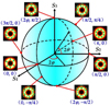 |
Fig. 1 Illustration of the Poincaré sphere, reprinted from Ma et al. (2022) under CC.BY 4.0. |
2.3 Closure quantities
Closure quantities are quantities that are derived from the observed visibilities. They are constructed in a way that they are independent of gain and/or leakage corruptions. Closure phases and closure amplitudes were used for a long time for total intensity imaging in VLBI. Closure phases are the phase derived over a triangle of antennas:
 (11)
(11)
Closure amplitudes are defined over a quadrilateral of antennas:
 (12)
(12)
Closure phases and closure amplitudes are independent of the gains, and thus have been used for closure-only imaging in the past (Chael et al. 2018; Blackburn et al. 2020; Arras et al. 2022; Müller & Lobanov 2022; Müller et al. 2023).
Closure traces could be understood as the polarimetric counter-part of closure amplitudes (Broderick et al. 2020a). They are defined over a quadrilateral of antennas as
 (13)
(13)
It can be seen now that Tri,j,k,l is independent of Ji, Jj, Jk, and Jl (i.e., independent of gains and leakage terms; Broderick et al. 2020a). On one quadrilateral with four different antennas i ≠ j ≠ k ≠ l, there are 24 permutations of i, j, k, l. However, only six out of these combinations are independent. These are (for a proof and more details, see Broderick et al. 2020a)
![Mathematical equation: $C{T_{i,j,k,l}} = \left[ {\matrix{ {T{r_{i,j,k,l}},T{r_{i,j,l,k}},T{r_{i,k,j,l}},T{r_{i,k,l,j}},T{r_{i,l,j,k}},T{r_{i,l,k,j}}} \cr } } \right].$](/articles/aa/full_html/2024/09/aa50437-24/aa50437-24-eq18.png) (14)
(14)
While closure phases and closure amplitudes have been directly fitted for total intensity imaging, closure traces have not been used as a calibration-independent data product that gets directly fitted by an imaging algorithm. However, there are first attempts to fit closure traces by model-fitting (Albentosa-Ruiz & Marti-Vidal 2023), and the analysis of closure traces have played a crucial role in the pre-imaging analysis of EHT datasets (Event Horizon Telescope Collaboration 2021a; Event Horizon Telescope Collaboration 2023). This may be caused by a number of degeneracies inherent to closure traces. As closure phases and closure amplitudes, they do not contain the absolute position, and the total flux of the image. However, the information regarding the relative information of structural features, their relative flux and the relative polarization signal remains preserved (as recently demonstrated by Albentosa-Ruiz & Marti-Vidal 2023). Particularly, closure traces are independent of any rotation on the Poincaré sphere (Broderick et al. 2020a); this is a special case, in which absolute EVPA (electric vector position angle) information is lost (rotations along the equator of the sphere). However, rotations on the Poincaré sphere also include rotations in latitude, mixing up linear polarization and circular polarization, compare Fig. 1.
Closure traces are defined on quadrilaterals. They will be the main focus of this manuscript due to their widespread use within the EHT collaboration. However, an alternative concept defined on closure triangles has been developed recently as well (Thyagarajan et al. 2022; Samuel et al. 2022). This concept builds invariants by triangles to a central station, and processing the Minkowski product of the four associated vectors.
3 Imaging
3.1 Overview
Imaging has been historically performed by the CLEAN algorithm and its variants (Högbom 1974; Clark 1980; Schwab 1984; Bhatnagar & Cornwell 2004; Cornwell 2008; Rau & Cornwell 2011; Offringa & Smirnov 2017; Müller & Lobanov 2023b). Recently forward modeling techniques have been proposed for VLBI as an alternative, especially for the EHT. These can be grouped into various categories: Bayesian reconstruction algorithms (Broderick et al. 2020b; Tiede 2022; Arras et al. 2022), RML approaches (Akiyama et al. 2017b,a; Chael et al. 2018), compressive sensing (Müller & Lobanov 2022), multi-objective imaging (Müller et al. 2023), and swarm intelligence (Mus et al. 2024a). Most of the aforementioned algorithms have been extended successfully to the polarimetric domain (Chael et al. 2016; Broderick et al. 2020b; Tiede 2022; Müller & Lobanov 2023a; Mus et al. 2024b,a). While the imaging algorithms are implemented in a variety of softwares, and differ significantly in the way the image is represented and regularization is perceived, all the forward modeling techniques have a relative modularity in common making it easy to extend the imaging algorithms to new data terms.
In this manuscript, we study the direct imaging from closure traces from the perspective of RML methods, although Bayesian frameworks may be equally well qualified as long as they support multimodal posterior exploration (in contrast to, e.g., resolve; Arras et al. 2022). This is the first direct imaging attempt from the closure traces. To study how restricting closure traces are, and what imaging strategies may be needed, we studied two competitive, alternative approaches.
First we utilized the numerically expensive multi-objective imaging algorithm MOEA/D recently proposed by Müller et al. (2023) and extended to polarimetric, and time-dynamic reconstructions in Mus et al. (2024b). MOEA/D uses the full set of common RML regularization terms (as they were applied in Event Horizon Telescope Collaboration 2021a), and searches for the front of Pareto optimal solutions among them. Among all RML approaches, MOEA/D may be most suited to study calibration-independent imaging, since instead of a single (maximum a posteriori) solution, a list of locally optimal solutions is found. In this way, MOEA/D may identify degeneracies, possibly multi-modality and non-convexity. MO-PSO, proposed by Mus et al. (2024a), is a variant of MOEA/D based on particle swarm optimization that does not explore the full Pareto-front, but solves several limitations of MOEA/D and improves over MOEA/D in accuracy.
Second, in contrast to MOEA/D, we utilized a lightweight alternative: DoG-HiT (Müller & Lobanov 2022). DoG-HiT represents the image by wavelets that are fitted to the uv coverage (Müller & Lobanov 2022, 2023b) and has been extended to polarimetry and dynamics (Müller & Lobanov 2023a). All RML regularization terms are replaced by a single, wavelet-based, reg-ularizer. In this way, DoG-HiT, contrasting MOEA/D, represents a simpler, automated alternative with weaker and data-driven regularization information.
By studying the closure-trace imaging from these perspectives, we covered the spectrum of RML methods along relatively weak prior assumptions (DoG-HiT) and relatively strong prior information (MOEA/D), which allowed us to identify the future prospects of imaging directly with the closure traces. We summarize in Appendix A the essential outline of the imaging algorithms MOEA/D, MO-PSO, and DoG-HiT. For more details we refer the reader to the respective references therein, especially Müller & Lobanov (2022) for DoG-HiT, Müller et al. (2023) and Mus et al. (2024b) for MOEA/D, and Mus et al. (2024a) for MO-PSO.
3.2 Imaging procedure
We recall from Sect. 2.3, and particularly the discussions in Broderick et al. (2020a), that closure traces have a variety of internal degeneracies. The most problematic one for a direct imaging from the closure traces is their property of being independent of any rotation in the Poincaré sphere. While closure traces are independent of any global rotation, their relative position across the image remains kept. In the case of negligible circular polarization, this rotation invariance translates into a degree of freedom in the overall EVPA orientation that could be calibrated effectively by accompanying observations on calibrator sources (e.g., see the strategy applied in Albentosa-Ruiz & Marti-Vidal 2023). This degeneracy (lost global EVPA orientation) is described by the rotations around the equator of the Poincaré sphere. However, if significant circular polarization is detectable in the source of interest, rotation invariance around the latitude could easily mix up linear polarization and circular polarization. We therefore restricted ourselves in this work to situations with negligibly small circular polarization at first instance. Among the rotation invariance, additional, potentially more complex degeneracies could arise, which would need to be taken into account during the imaging.
Compared to using the full set of visibilities, any kind of closure quantity represents just a subset of observables. This contributes to the sparsity of the observation, and ultimately worsens the situation of an only weakly constraining dataset. In the case of closure traces, they are a statistically complete set of all gain- and d-term-independent quantities. It has been demonstrated in the past that imaging from closure products only, at least in total intensity, is still feasible when powerful regularization frameworks are used. This has been originally demonstrated for RML imaging in Chael et al. (2018), and was subsequently utilized in a wide range of imaging approaches in the context of the EHT including Bayesian reconstructions (Arras et al. 2022), compressive sensing (Müller & Lobanov 2022), and multi-objective imaging (Müller et al. 2023).
Finally, non-convexity may be a potential issue for the imaging. Strict convexity of the objective is a sufficient condition to prove uniqueness of an optimization, and a single-mode posterior. The opposite is not necessarily true: a non-convex optimization problem does not necessarily need to be multimodal, but is prone to be so in practice. The χ2 metric to the closure traces is not strictly convex. This is easily proven by the existence of a flat plateau along the rotation-invariance around the Poincaré sphere, as discussed above. However, we cannot analytically prove that there is a definitely concave part of the objective.
In any case, these three limitations (inherent degeneracies, a smaller number of independent observables, and a potentially non-convex optimization problem) pose serious issues for local search methods, which, as a consequence, may be trapped in local extrema rather than searching for the global optimum. Multi-objective optimization, and particularly MOEA/D (Müller et al. 2023), are a good alternative. Due to their randomized search techniques they navigate the objective landscape more globally. Particularly, the various clusters of Pareto optimal solutions identified by MOEA/D both in total intensity, as also in polarimetric reconstructions (Mus et al. 2024b) are interpreted as lists of locally optimal modes. Therefore, we used MOEA/D.
The set-up of MOEA/D for the reconstruction with respect to closure traces consists of solving a multi-objective problem with the following objective functionals (inspired by the parametrization proposed in Mus et al. 2024b):
 (15)
(15)
 (16)
(16)
 (17)
(17)
 (18)
(18)
Here we used the χ2 statistics of the array of six independent closure traces, CT (see Eq. (14)) as the data term. The regularization terms are polarimetric variants of the entropy Rms, Rhw and the polarimetric counterpart of the total variation regularizer Rptv. The exact regularization terms can be retrieved by Appendix B.
The specific challenges posed by directly fitting the closure traces made a couple of additional updates to the imaging pipeline of MOEA/D necessary that are detailed in Appendix C.
4 Synthetic data tests
We tested the potential for closure trace imaging in a variety of settings and along multiple axes with targeted tests. We studied whether the imaging works in general and is competitive with classical approaches, and how that assessment changes with the sampling of uv-domain, and methodology used.
4.1 Synthetic data
To this end, we performed the synthetic data tests with the configuration of the EHT in 2017 and with a proposed configuration of the next-generation EHT (ngEHT) taken from the ngEHT analysis challenge (Roelofs et al. 2023a). The latter was selected since the corresponding datasets and data properties have regularly been used to verify and validate novel imaging algorithms. The array consists of all the current EHT antennas and ten additional stations taken from the list of Raymond et al. (2021). We compare the corresponding uv coverages in Fig. 2.
We tested three synthetic ground truth models. One model is a geometric model that has similar properties as the EHT observations of M87 in polarization (Event Horizon Telescope Collaboration 2021a). It consists of a ring with a diameter of 41 µas, and a compact flux of 0.6 Jy. The EVPA pattern is a radial pattern twisted by 45 degrees. The model is equivalent with the geometric ring model with a vertical magnetic field that was tested in Mus et al. (2024b).
As an additional test source, we used the result of a general relativity magnetohydrodynamic (GRMHD) simulation of SgrA* that is commonly available in the ehtim software pack-age1. The model mimics the typical crescent-like appearance of SgrA* in EHT observations, with a polarimetric pattern that differs around the ring, consequently covering a different test case than the first model.
Finally, we tested a non-ring mode. To this end, we developed a synthetic dataset inspired by the observation of 3C279 with the EHT (Kim et al. 2020) that essentially resembles a double source with reshaped elongated Gaussians. The ground truth image is constructed out of six Gaussian components (C0-0, C0-1, C0-2, C1-0, C1-1, and C1-2) with the amplitudes and relative positions that were reported from the geometric model-fitting results shown in Kim et al. (2020) for April 5. We separated the two clusters and added linear polarization synthetically with an EVPA pattern roughly aligned with the expected jet axis in 3C279 (Kim et al. 2020).
The synthetic observations were performed with the EHT and the EHT+ngEHT configuration. To this end, we downloaded the true observations done with the EHT on April 11, 2017 (Event Horizon Telescope Collaboration 2019b) from the public release page of the EHT2, as well as the synthetic ground truth dataset used in the ngEHT analysis challenge3 for M87. For the synthetic SgrA* reconstructions, we downloaded the respective observation files on SgrA* from the same web pages4. The synthetic observations were performed by the ehtim package. This routine basically reads the uv coordinates, and respective thermal noise level, from an existing observation file, evaluates the Fourier transform of the ground truth model at these spatial frequencies, and adds thermal noise. This is a rather simplistic forward model, and we would like to note the existence of more complex simulation tools that were developed within the EHT collaboration (e.g., Roelofs et al. 2020) that mainly model tropospheric effects in richer detail. In the case of SgrA*, we ignored the effects of the scattering for now; for example, we did not apply a strategy of inflating the noise levels as was done by the EHT (Event Horizon Telescope Collaboration 2022). Since the synthetic observations mimic the systematic noise levels of previously reported real and synthetic datasets, we refer the reader to Event Horizon Telescope Collaboration (2019a), Event Horizon Telescope Collaboration (2022), and Roelofs et al. (2023a) for more details on the data properties. For the original EHT+ngEHT datasets simulated by Roelofs et al. (2023a), we assumed a bandwidth of 8 GHz and a receiver temperature of 60 K with an aperture efficiency of 0.67 at 230 GHz. The opacity values were extracted as the median of the estimates reported by Raymond et al. (2021) at an elevation of 30 degrees (Roelofs et al. 2023a).
We added gain corruptions and d-term corruptions to the observations. The d-terms were perturbed by a mean of 5% on all baselines, not taking typical d-term signatures for the EHT into account (for instance, the fact that d-terms for ALMA are typically only imaginary). In any case, these corruptions do not affect the closure traces at all, and the imaging remains robust against gain and d-term corruptions. We scan-averaged the data and rescaled the inter-baseline fluxes to the correct total flux before forming closure triangles and closure quadrangles. A systematic noise budget of 2% was added to the data on all baselines before reconstruction.
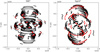 |
Fig. 2 Illustration of the uv coverage of M87 (left panel) and SgrA* (right panel) with the EHT array of 2017 (red points) and the proposed EHT+ngEHT configuration (black points; Roelofs et al. 2023a). |
4.2 Reconstruction results
We show the reconstruction results in Fig. 3. We compare the reconstructions with MOEA/D only fitting to closure traces for the EHT, with the EHT+ngEHT configuration, and with a reconstruction that directly fits the (non-calibrated for leakages) Stokes visibilities. The last reconstruction just assumes that the emission in total intensity, and the polarized emission share similar spatial scales and support (e.g., have a similar size of the compact emission). No explicit regularization terms on the polarized emission, such as a polarized entropy or smoothness assumptions, are used. Thus, it represents a rather weak prior information that does not process the closure traces. We did not fit d-terms, so the reconstruction shows the effects of a missing d-term calibration in comparison to a d-term-independent reconstruction.
The reconstruction with the EHT+ngEHT configuration is rather successful in both cases. The reconstructions look more scrambled in the reconstruction than in the ground truth. In Fig. 4 we show the reconstructions blurred with the nominal beam resolution (20 µas). This comparison at lower resolution shows that the scrambled, noisier reconstruction seems to be an effect of the reconstruction of super-resolved structures.
While the EHT+ngEHT configuration allows for good reconstruction results, the EHT observations with a much sparser uv coverage are less successful. This is understandable giving the much smaller number of antennas. The EHT observations did use seven antennas. Additionally, one antenna (JCMT) needed to be flagged for the closure trace analysis, since only one polarization channel is available. Moreover, two antenna pairs (ALMA/APEX and JCMT/SMA) are essentially at the same position. Hence, the number of quadrilaterals that resolve structure is small for the EHT configuration. In fact, the EHT reported only one quadrilateral with a sufficient signal-to-noise ratio to draw conclusions (Event Horizon Telescope Collaboration 2021a; Event Horizon Telescope Collaboration 2023).
Since the imaging is independent of any kind of d-term, this challenging analysis step can be omitted. However, at a backside, the number of independent observables drops, making the imaging more challenging. The imaging directly with closure traces is only a valid methodology, if the loss in sensitivity is smaller than the loss in accuracy introduced by the d-terms. Comparing the second and last column in Figs. 3 and 4, this seems to be the case qualitatively. We present a closer look at this property in Sect. 4.5.
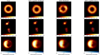 |
Fig. 3 Comparisons of three different source structures (ring inspired by Event Horizon Telescope Collaboration 2021a, a double source mimicking Kim et al. 2020, and a GRMHD model of SgrA*) and their corresponding reconstructions. First column: Ground truth. Second and third column: Reconstructions with closure trace imaging with MOEA/D with two different array configurations. Fourth column: Direct reconstruction with DoG-HiT with 5% of residual (not corrected) leakages as a comparison. |
4.3 Pareto fronts
Next we took a closer look at the Pareto fronts. The Pareto fronts are presented in Appendix D. We show the Pareto fronts in Figs. D.1, D.2, and D.3 for the ring model. MOEA/D finds a number of clusters representing locally optimal modes. The clusters 0, 1, and 2 are dominated by the polarimetric total variation and lie at the edge of the parameter space, and hence do not describe the ground truth image properly. However, there are two clusters with well scoring with respect to the closure traces. Interestingly, they do describe two different radial EVPA patterns, describing two different local minima that a local search technique may fall into. MOEA/D succeeds in sampling both, and thus describes the range of possible image structures.
In practical situations, we do not know the ground truth image. Müller et al. (2023) and Mus et al. (2024b) developed two different approaches to selecting the objectively best image. A selection by the accumulation point of the Pareto front, or by the cluster that is closest to the utopian ideal point proved successful in practice, both for total intensity as well as for polarimetric reconstructions. Especially the distance to the ideal point was then used in Mus et al. (2024a) as the objective criterion for particle swarm optimization. We mark the solution that is closest to the ideal by a red box in Figs. D.1, D.2, and D.3. The selection criterion selects the best image, the same is true for the double source and the GRMHD example as well (see Figs. D.4 and D.5).
In the case of closure traces, there is furthermore an alternative possible concept for the selection. Since two different concepts for closure products exist, closure traces defined on quadrilaterals (Broderick et al. 2020a) and closure invariants defined on closed triangles by gauge theory (Thyagarajan et al. 2022; Samuel et al. 2022), one could try to retrieve the best cluster by the scoring in the triangle based closure invariants. Although closure traces are a complete set of closure products, the closure triangle version defined by Thyagarajan et al. (2022) and Samuel et al. (2022) may package this information in a different way. A different packaging of in principle equivalent information in the data fidelity term could impact the reconstruction in a RML framework, at least due to the locality of the optimization methods. Furthermore, the noise distribution on the closure triangles and closure quadrangles is only known approximately, and differs between the triangle relations and quadrangle relations. Therefore, a cross-validation may find the best reconstruction. We mark the cluster selected by the best fit to closure triangles with a dashed blue box. However, this selection fails. This may be explained by the fact that both closure invariants form a full set of invariant properties, and encode the same amount of information consequently, making a cross-verification not the correct tool for selecting the best cluster.
 |
Fig. 5 Ground truth image compared to various realizations of directly fitting closure traces for the EHT+ngEHT configuration. Second column: Reconstruction by MOEA/D only fitting closure traces. Third column: Reconstruction by MO-PSO only fitting closure traces. Fourth column: Reconstruction by MO-PSO fitting closure traces and visibilities. |
 |
Fig. 6 Same as Fig. 5, but for the EHT configuration. Additionally, we show in the fifth column a direct reconstruction from the visibilities when leakages at a level of 5% are not corrected. |
4.4 MO-PSO
The selection of the best cluster discussed in Sect. 4.3 suggests that the selection of the most natural cluster by the smallest distance to the ideal point works. This distance was proposed as the objective functional for MO-PSO (Mus et al. 2024a). MO-PSO presents some advantages over MOEA/D. Since the evolutionary algorithm is only used to explore the weights space, but not to recover the actual image from the visibility data, it is orders of magnitude faster than MOEA/D. MO-PSO does not recover the full set of local extrema as MOEA/D (which was identified crucial for this application), but it still searches the objective landscape globally and converges to the same preferred cluster as MOEA/D (since the selection criterion is used as an objective functional). Based on the analysis presented in the previous subsection, MO-PSO is also applicable for the problem of recovering polarimetric images directly from the closure traces.
We show in Fig. 5 the reconstruction result of MO-PSO for the EHT+ngEHT configuration, and in Fig. 6 the performance for the EHT array alone. The reconstructions with MO-PSO and MOEA/D do not differ by much, and the latter was much faster. In conclusion, since multiple clusters have been identified with MOEA/D, global search techniques should be preferred over local search techniques. However, the success of MO-PSO for a denser array configuration indicates that the full Pareto front does not need to be sampled, rather the most natural solution is preferred.
 |
Fig. 7 Impact of residual leakage compared to the leakage-independent imaging from the closure traces by MOEA/D. Top row: ground truth image, direct imaging result when leakages are perfectly recovered, and closure trace fitting result from MOEA/D. Middle and bottom row: direct reconstruction results with increasing levels of residual leakage errors (which are not calibrated out of the observation). |
4.5 Effect of leakage inaccuracies
Imaging directly from the closure traces has the significant advantage of being independent of any gain and leakage corruptions. However, as a disadvantage, the related optimization problem is more complex and has several potential degeneracies. In this subsection, we discuss at what point the advantages start to outweigh the disadvantages. To this end, we ran a targeted test on the ring model with the EHT+ngEHT coverage. We recovered the polarimetric result directly with DoG-HiT, adding no d-term corruptions, and adding 1%, 2%, 5%, 10%, 20%, and 30% (residual) leakage corruptions. In reality someone would estimate the leakages based on the total intensity image or together with it. However, this reconstruction is subject to inaccuracies as well, which may lead to residual leakage errors that are passed down to the polarimetric imaging. Here we took the size of the residual leakages that were not successfully calibrated into account in contrast it to the reconstruction done by closure trace imaging. To this end, we did not calibrate the leakages that we added to the data, and therefore estimated the impact of 1%, 2%, 5%, 10%, 20%, and 30% residuals leakages after calibration rather than the effect of this size of leakages in general. In this way, we could explicitly quantify the effect of corrupted (or not fully calibrated) leakages on the fidelity of the image reconstruction. We evaluated the reconstructions with the cross-correlation between the ground truth and the recovered solution for P = Q + iU that was proposed in Event Horizon Telescope Collaboration (2021a). The results are plotted in Fig. 7.
As expected, the direct reconstruction with DoG-HiT with the synthetic data, which are corrupted by thermal noise and complex gains buthave the correct d-terms, performs bestamong all reconstructions. In the second and third column we identify the effect of dropping accuracy in the d-terms. As expected, the cross-correlation between the ground truth image and the recovered images decreases with increasing level of perturbations. The MOEA/D reconstruction becomes competitive for d-term inaccuracies of roughly 2%. This is indeed a typical size of inaccuracies in the determination of d-terms. If the residual d-terms after calibration are larger than 5%, the inaccuracy in the polarimetric calibration dominates the drop in independent observables.
4.6 Stabilizing direct imaging
Finally, we discuss the prospects of stabilizing the direct imaging from the Stokes visibilities with a fit to the closure traces. To this end, we used MO-PSO but added the χ2 statistics to the vector of objectives as a fifth objective. Now the multi-objective optimization problem consists of three regularization terms (Rhw, Rms, Rptv) and two data terms  . The respective reconstruction result is shown in the last column of Figs. 5 and 6.
For the EHT+ngEHT configuration at which the dataset is very constraining on its own only minor improvements are detected. The EHT configuration shows an interesting behavior. The direct imaging to the uncalibrated d-terms and the simple fit to the closure traces do not produce a good reconstruction.
If both observables are combined, however, the reconstruction performs well.
 |
Fig. 8 Ring model (left panel) recovered with MOEA/D and MO-PSO (including polarimetric visibilities) and the 2021 configuration (second and third panel). For comparison, we reprint the reconstruction results in the EHT 2017 array in the last two panels. |
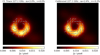 |
Fig. 9 Reconstructions on real data observed in 2017 by the EHT. Left panel: Reconstruction achieved by directly fitting closure traces with MO-PSO. Right panel: Reconstruction when fitting the Stokes visibilities with DoG-HiT, with the leakage already calibrated. |
4.7 Dependence on data quality
In this manuscript we mainly discuss and compare two different settings, namely the setting of the EHT in 2017, and a much denser array proposed for the EHT+ngEHT. The results presented in the previous subsections suggest that directly fitting the closure traces, either with MOEA/D or MO-PSO, allows for reasonable reconstructions in the setting for the EHT+ngEHT comparable to the reconstruction with residual leakage errors of a few percent. However, as can be seen for example by comparing the reconstructions obtained with the EHT in Fig. 6 and the EHT+ngEHT setting in Fig. 5, or the middle left and middle right columns in Fig. 3, the reconstruction is very challenging for the EHT configuration of 2017, and largely unsuccessful except for the case of stabilizing the fit to the polarimetric visibilities with the closure traces as discussed in Sect. 4.6.
In this subsection, we discuss an intermediate configuration, namely an observational setting that may be expected from the 2021 EHT array. This array contains of the 2017 EHT array as well as the Greenland Telescope (which joined in 2018 and significantly improved the coverage in the north-south direction; Event Horizon Telescope Collaboration 2024), the 12m telescope at Kitt Peak, and NOEMA (which joined in 2021). To this end, we reused the EHT+ngEHT simulation, and flagged all baselines not in the 2021 array.
We show the reconstruction results comparing to the 2017 EHT observations discussed earlier in Fig. 8. From this short analysis, we can conclude that the direct fitting to the closure traces may already be a viable option with the current EHT array (i.e., with the configuration in 2021).
5 Real data application
Most of the tests done in this work reside around synthetic EHT data. Finally, we tested the procedure on existing, real observations. We applied our algorithms to the public calibrated M87 observations of the EHT on April 11, 20175. However, we recall our conclusions that it is challenging to emulate a consistent polarimetric image of M87 with the EHT coverage of 2017 from the closure traces alone with our procedure (compare the reconstructions shown in Figs. 3 and 6). Therefore, we also chose a different test dataset with the aim to reproduce the numerical experiment performed in Albentosa-Ruiz & Marti-Vidal (2023), pioneering work that directly fitted closure traces.
We show in Fig. 9 the reconstruction with real data. The left panel shows the reconstruction with MO-PSO. In the right panel we show as a comparison the reconstruction done with DoG-HiT when fitting polarimetric visibilities instead. We note that in the latter case the leakage terms, the main cause of issues closure trace imaging is designed to be robust against, were corrected by the detailed and vetted estimates obtained by the EHT (Event Horizon Telescope Collaboration 2021a). That means that the DoG-HiT reconstruction has been obtained from the already calibrated data.
Both reconstructions recover similar overall azimuthal patterns, as did the EHT collaboration (Event Horizon Telescope Collaboration 2021a; Event Horizon Telescope Collaboration 2021b). The reconstruction done on the calibrated data, however, is more regular and less noisy, likely due to the higher signal-to-noise ratio in the visibility data compared to the closure traces, whose information content is reduced in comparison to the visibilities.
Albentosa-Ruiz & Marti-Vidal (2023) analyze the observations of M87 that were observed with ALMA during the EHT campaign in 2017 (Event Horizon Telescope Collaboration 2019b), on April 6. The observations were performed in ALMA Band 6, with an array of 33 antennas covering baseline lengths between 15.1 m and 160.7 m. Albentosa-Ruiz & Marti-Vidal (2023) studied four spectral windows, at frequencies of 213.1 GHz, 215.1 GHz, 227.1 GHz, and 229.1 GHz. For this work, we reproduced the image at the third spectral window (227.1 GHz), matching the lower band of the EHT observations.
The ALMA observations are high signal to noise reconstructions on a large number of antennas. We remind ourselves that the information loss by the use of closure trace instead of visibilities – for example the number of statistically independent closure traces to the number of statistically independent visibilities – converges to one with the number of available antennas (Broderick et al. 2020a). Hence, a proper reconstruction performance is expected. We wish to highlight that this application is one of the first applications of the family of closure-only imaging algorithms developed for the EHT to non-EHT data. This is particular interesting for wide-field, wideband interferometric imaging at which the polarization dependence of the primary beam is taken into account by projection algorithms approximately (Bhatnagar et al. 2013). In this work, we focused on the simpler problem of reproducing the modeling results presented in Albentosa-Ruiz & Marti-Vidal (2023) instead, and leave the discussion of bypassing antenna-based primary beam pattern for a consecutive work.
The data were downloaded from the ALMA archive and calibrated with the ALMA pipeline script. We exported the measurement sets to the uv fits format and time-averaged the data by 10 seconds, and performed the reconstruction with the software tool MrBeam6. The pipeline product of ALMA was used as an initial guess. The reconstruction of the polarized structure from the closure traces, was then performed with the MO-PSO algorithm that performs much faster than MOEA/D. Due to the larger number of pixels and the larger number of visibilities, this speed-up proved to be essential to ensuring a timely numerical performance.
We show the recovered polarization structure in Fig. 10. The Stokes I reconstruction, as well as the EVPA structure looks very similar to the reconstructions presented in Albentosa-Ruiz & Marti-Vidal (2023), presenting an interesting cross-verification. We would like to note that the approach presented in this manuscript differs significantly from the approach pioneered by Albentosa-Ruiz & Marti-Vidal (2023), who used a model-fitting approach and explored the model-fitting components with a full Markov chain Monte Carlo approach. We, on the other hand, studied the direct imaging with multi-objective optimization. Given these philosophically differences in the way the problem is approached, the significant similarities in the reconstructions serve as a powerful consistency check of the procedure described in this manuscript. Finally, we would like to note that Albentosa-Ruiz & Marti-Vidal (2023) found multiple modes describing the data when performing a full gridded exploration of the χ2 parametric space. While we do not reproduce the multi-modality of the problem setting since we used MO-PSO instead of MOEA/D (which would explore the full Pareto front), MO-PSO seems successful in navigating this challenging parametric space due to its evolutionary approach.
The reconstruction was performed on a common notebook in roughly 30 minutes. This highlights the scalability of the MO-PSO algorithm to existing datasets, and the applicability of procedures that were initially proposed for the EHT in a more general setting.
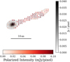 |
Fig. 10 Reconstruction of ALMA Band 6 observations of M87 at 227.1 GHz. |
6 Conclusions
Closure traces (Broderick et al. 2020a) extend the well-known closure phases and closure amplitudes to the polarimetric domain. One of their key features is that they are independent of gain corruptions and leakages, making them an important closure quantity for studying the polarimetric signature of a source. This is particularly true for the EHT and its planned successors (e.g., the EHT+ngEHT) due to the relative sparsity of the observation, the low signal-to-noise ratio, and the huge gain uncertainties. We have evaluated, using some exemplary studies, whether closure traces can be used as a data functional in the same way that closure phases and closure amplitudes are used for closure-only imaging. This operational mode may prove to be particularly important due to the potential lack of suitable calibrators with sufficient parallactic angle coverage, or a lack of unresolved calibrator sources at all. A first pioneering work in this direction is presented by Albentosa-Ruiz & Marti-Vidal (2023), albeit in a model-fitting setting rather than one that involves direct imaging. Here, we studied the imaging problem instead.
To this end, we constructed an imaging strategy that explicitly deals with the degeneracies and potential multi-modality that are associated with closure traces. In a nutshell, we utilized the multi-objective imaging methods MOEA/D (Müller et al. 2023; Mus et al. 2024b) and MO-PSO (Mus et al. 2024a), which approximate multiple local minima simultaneously. Multiple local minima that would pose significant challenges for local search techniques were identified (including the rotation invariance around the Poincaré sphere).
We applied our imaging pipeline to three different synthetic datasets that resemble usual EHT targets, in two different array configurations and with various levels of noise corruption. As a remaining limitation, we relied on the assumption of vanishing circular polarization, which may not be justified for the main targets of the EHT (Event Horizon Telescope Collaboration 2023).
This application demonstrated that the closure traces, while putting reliable upper limits on the polarization fraction (Event Horizon Telescope Collaboration 2021a; Event Horizon Telescope Collaboration 2023), are not informative enough for the EHT to allow for polarimetric imaging. This is consistent with the conclusions drawn by the EHT collaboration (Event Horizon Telescope Collaboration 2021a) and is mainly caused by the small number of quadrilaterals that probe extended structural information with a sufficient signal-to-noise ratio.
A planned successor of the EHT, the EHT+ngEHT (which could have ten additional antennas), will have a much larger number of quadrilaterals. Closure trace imaging will become a feasible alternative in this configuration and will produce competitive results with residual leakages at a few percent level. Similarly, the EHT configuration of 2021 could potentially also be used to produce a statistical set large enough to apply this technique.
Although the data are more constraining with the additional antennas assumed in this work, the Pareto front recovered by MOEA/D still features multiple prominent clusters. This may be due to the existence of multiple local minima, which (depending on the starting point) a local search technique could fall into. The cluster that is closest to the utopian ideal (as proposed by Müller et al. 2023; Mus et al. 2024a) contains the best solution. This supports the use of MO-PSO, which is a faster alternative to MOEA/D and utilizes the distance to the ideal as its objective functional.
To complement these tests on synthetic data in an EHT setting, we applied the pipeline to real observations of M87 from ALMA. The recovered structure is similar to the model-fitting approach presented in Albentosa-Ruiz & Marti-Vidal (2023), further substantiating the robustness of the data analysis pipeline from the closure traces alone presented in this manuscript. Moreover, this application demonstrates the scalability of MO-PSO to less sparse, highly dynamic range datasets, and contributes to a line of recently initiated research that is evaluating the usefulness of the data analysis techniques proposed by the EHT in a more general setting.
We conclude that closure trace imaging will be a feasible and competitive alternative to the classical hierarchical VLBI imaging, or the simultaneous reconstruction of gains and d-terms together with the image structure explored by Bayesian methods, at least in numerical practice when theoretical marginalization over the unknown gains and leakage terms can include nontrivial approximations. In this manuscript, we have laid out the strategy of how to implement this philosophy in practice. Finally, closure trace imaging does not need to be applied independently: a short analysis shows that it may also improve the RML imaging pipeline when applied together with classical polarization data terms.
Acknowledgement
This work was partially supported by the M2FINDERS project funded by the European Research Council (ERC) under the European Union’s Horizon 2020 Research and Innovation Programme (Grant Agreement No. 101018682). HM received financial support for this research from the International Max Planck Research School (IMPRS) for Astronomy and Astrophysics at the Universities of Bonn and Cologne, and through the Jansky fellowship awarded by the National Radio Astronomy Observatory. The National Radio Astronomy Observatory is a facility of the National Science Foundation operated under cooperative agreement by Associated Universities, Inc. This paper makes use of the following ALMA data: ADS/JAO.ALMA#2016.1.01154.V ALMA is a partnership of ESO (representing its member states), NSF (USA) and NINS (Japan), together with NRC (Canada), MOST and ASIAA (Taiwan), and KASI (Republic of Korea), in cooperation with the Republic of Chile. The Joint ALMA Observatory is operated by ESO, AUI/NRAO and NAOJ. The data underlying this work are accessible from the ALMA data archive, synthetic datasets will be shared upon reasonable request. The software used to produce these results is MrBeam, publicly available through github (https://github.com/hmuellergoe/mrbeam). MrBeam makes explicit use of the following packages: ehtim (https://achael.github.io/eht-imaging/), WISE (https://github.com/flomertens/wise), regpy (https://num.math.uni-goettingen.de/regpy/) and pygmo (https://esa.github.io/pygmo2/).
Appendix A Description of the imaging algorithms
A.1 MOEA/D
RML imaging algorithms minimize a sum of data fidelity terms and regularization terms. By minimizing a weighted sum of these terms, one tries to find a solution that is favorable both by the data fidelity terms and the regularization terms, namely, a solution that fits the observed data and is physically reasonable. There are multiple regularization terms that are commonly used for VLBI and represent a wide variety of prior assumptions, for example the simplicity of the solution (measured for example by the entropy Rentr or the l2 norm  ), the sparsity (l1 norm
  ), the smoothness (total squared variation Rtsv, total variation Rtv), or the correct total flux. We refer the reader to Müller et al. (2023) and Event Horizon Telescope Collaboration (2019a) for a discussion of the full range of regularization terms.
For MOEA/D, the whole range of reasonable image features that may be fitted to the data with a specific regularization parameter weight combination is searched by multi-objective evolution where every data term and regularization term is modeled as an individual objective (Müller et al. 2023).
MOEA/D recovers the Pareto front consisting of all Pareto optimal solutions by the genetic algorithm (Zhang & Li 2007; Li & Zhang 2009). A solution is called “Pareto optimal” if the further optimization along one of the objectives has to worsen the scoring in another objective; for example, the further minimization of the χ2 metric has to worsen the entropy or sparsity assumption. In this way, MOEA/D succeeds at exploring the image structures globally, recovering all the locally optimal image structures along the objectively best.
It has been shown in Müller et al. (2023) that the Pareto front has a specific structure for an EHT-like configuration: it divides into multiple disjoint clusters, each of them representing a locally optimal mode. For more details we refer the reader to Müller et al. (2023) and Mus et al. (2024b) and references therein.
A.2 MO-PSO
MO-PSO was proposed by Mus et al. (2024a) as a companion to MOEA/D. It solves some of the numerical limitations of MOEA/D and improves the accuracy of the reconstruction. The Pareto front has an asymptotic behavior with regard to any axis (i.e., any individual objective). This is the scoring of any of the objective terms when only this objective plays a role in the reconstruction. The stacked asymptotic scoring in any of the objective terms is the ideal point (see Fig. A.1 for an illustrative sketch). It has been shown in Müller et al. (2023) and Mus et al. (2024a) that the distance between the ideal point and the scoring of the Pareto optimal solutions can be used to select the best reconstruction in the Pareto front.
MO-PSO uses this observation to define a convex optimization problem with respect to the weights. It tries to find the Pareto optimal image structure with the smallest distance to the ideal point (i.e., the closest optimum in Fig. A.1) by screening the regularization weights with a particle-swarm optimization algorithm, and solving the related weighted sum problem by fast gradient based minimization techniques. For more details, we refer the reader to Mus et al. (2024a). In a nutshell, every particle in the swarm represents a single weight combination. We solved the related weighted sum problem. This solution approximates a Pareto optimal solution. Next we computed the distance of this solution to the ideal point. Then we updated the position of every particle (i.e., the weight combinations) by the update step of a particle swarm optimization, solved for the related images, and accepted these updates if the distance to the ideal point improved.
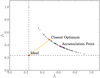 |
Fig. A.1 Illustrative sketch of the Pareto front in two dimensions, the construction of the ideal point using the asymptotic behavior along each single axis, and the distance to the Pareto front as a selection criterion. This distance is minimized by MO-PSO. The figure is reprinted from Müller et al. (2023) under CC.BY. 4.0.. |
A.3 DoG-HiT
DoG-HiT models the image structure by wavelets that are fitted to the uv coverage (Müller & Lobanov 2022). The image is recovered by standard sparsity promoting regularization. In this way, DoG-HiT effectively computes the multi-resolution support, which is the set of statistically significant wavelet coefficient that are needed to represent the image, inspired by Mertens & Lobanov (2015). It has been demonstrated in Müller & Lobanov (2023a) that the multi-resolution support is a reasonable prior for a full polarimetric (and time-dynamic) reconstruction. For the reconstruction of the polarimetric signal, we only varied the wavelet coefficients within the multi-resolution support and fit the Stokes visibilities directly; in other words, we solved the problem using a constrained minimization approach.
DoG-HiT is not the primary subject of the investigation in this manuscript. In this study, we fit directly to the closure traces with MOEA/D and MO-PSO. However, we used DoG-HiT as an initial guess for the total intensity structure and, as a comparison, an imaging algorithm. DoG-HiT is a good choice for a comparison of the performance, since it is philosophically close to the multi-objective approaches (i.e., it approaches the problem in a RML fashion, rather than by inverse modeling or Bayesian exploration), it is fast, unbiased in total intensity (fits only to closure phases and closure amplitudes), and, most importantly, it is automatized and unsupervised (e.g., see the discussion in Müller & Lobanov 2022). Particularly the last point makes it a reasonable choice as a comparison method, aiming at minimizing the human factor in the comparison. Moreover, the reconstruction of the linear polarization is straightforward and represents a relatively weak, but data-driven, prior assumption, opposed to the computationally expensive algorithms MOEA/D and MO-PSO that survey a variety of strong prior assumptions.
Appendix B Polarimetric regularization terms
The polarimetric regularizers used in this study are as follows: We used polarimetric variants of the image entropy as regularizers, as proposed by Narayan & Nityananda (1986):
 (B.1)
(B.1)
 (B.2)
(B.2)
Moreover, we used the polarimetric counterpart of the total variation regularizer (Chael et al. 2016):
 (B.3)
(B.3)
Here I denotes the total intensity, M the total intensity of a prior model, m the polarization fraction, and P = Q + iU the complex-valued linear polarization vector.
Appendix C Updates to the MOEA/D pipeline
In the following list we enumerate the detailed changes that needed to be done to the MOEA/D pipeline to allow for the reconstruction of the linear polarization signal directly from the closure traces:
We studied the prospects of using closure traces directly to fit in a self-calibration independent way the linear polarization signature, ignoring circular polarization for now, and not focusing on total intensity. Closure traces contain classical closure amplitudes and closure phases as a special case, and extend these concepts to the polarimetric domain. Instead of using closure traces only for the polarimetric signal, one could also try to recover the total intensity image by directly fitting closure traces. However, the total intensity imaging is only weakly affected by the leakages. The imaging in total intensities by closure properties has been intensively studied and has been shown to lead to reliable image reconstructions (e.g., Chael et al. 2018; Müller & Lobanov 2022; Arras et al. 2022; Müller et al. 2023; Thyagarajan et al. 2024). Hence, we focused on the reconstruction of the linear polarization features by fitting the closure traces, and recover the total intensity image by alternative closure-only imaging algorithms. For the test-cases presented here, we did the reconstruction of the total intensity image by DoG-HiT fitting directly closure amplitudes and closure phases.
Once the total intensity image has been successfully recovered, we moved to the polarimetric part. The polarimetric signal is represented by the polarization fraction, m, and the mixing angle, χ, for the polarimetric reconstruction rather than by Q and U. This equivalent re-parametrization allows the inequality (8) to be used in a more straightforward way, by rigidly setting bounds on the polarization fraction.
Originally, MOEA/D is initialized using either a completely random initial population or the result of an un-penalized imaging run with a few iterations. Müller et al. (2023) provide a comparison between these two initialization strategies. The first starts with a more global distribution of genomes across the parameter space, making it easy to recover the potentially multi-modality of the problem. The second strategy speeds up the reconstruction with MOEA/D with a starting point that is actually closer to the finally preferred solution. We opted for a hybrid way in this study. Since the un-penalized minimization varies significantly with the initial guess used, we used 11 random EVPA orientations, performed the un-penalized minimization, and initialized the initial population for MOEA/D by 91 copies of each, matching the overall population size 1001 genomes in the populations that is set by the combinatoric number of weightings λ with a fixed grid size that sum to one.
To avoid a situation in which, due to this random initialization, specific source solutions are related to specific weight combinations, we added a fifth functional (i.e., a fifth axis) to MOEA/D. This functional is constantly zero, so does not add anything up to the optimization at all, but serves as an axis to store multiple solution varieties originating from various starting points for the same weighting combination. Furthermore, we randomized the weight generation, λ, rather than drawing them from a grid as we did before.
Since closure traces are independent of any global rotation of the EVPA pattern, MOEA/D naturally samples the full domain of the global orientations, that is, the population contains genomes that only differ by an overall constant offset to the mixing angle χ. All the images that are equal up to a constant angle have the same scoring in the objective func-tionals since the regularizer terms are also independent of the overall orientation. To avoid this unnecessary duplication of information, we used an alternating procedure. We took the initial population, updated the population by a number of generations (set to ten), ordered the images in clusters as described in Mus et al. (2024b), and aligned all genomes within one cluster with respect to the overall EVPA orientation. Then we initialized the next population with the aligned genomes and proceeded with the genetic evolution. This procedure was repeated multiple times.
Appendix D Pareto fronts
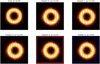 |
Fig. D.1 Pareto front of the MOEA/D reconstruction directly fitting to closure traces for the EHT+ngEHT array configuration. The solution in the red box is preferred by MOEA/D as the Pareto-optimal solution closest to the optimum; the cluster with the blue box would have been selected when comparing to closure quantities defined in Thyagarajan et al. (2022) and Samuel et al. (2022). |
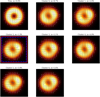 |
Fig. D.3 Same as Fig. D.1, but for the EHT array configuration. Additionally, a blurring of 20 µas has been applied to every cluster. |
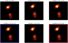 |
Fig. D.4 Pareto front of the double source in the EHT+ngEHT configuration. |
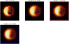 |
Fig. D.5 Pareto front of the SgrA* source model in the EHT+ngEHT configuration. |
References
- Akiyama, K., Ikeda, S., Pleau, M., et al. 2017a, AJ, 153, 159 [NASA ADS] [CrossRef] [Google Scholar]
- Akiyama, K., Kuramochi, K., Ikeda, S., et al. 2017b, ApJ, 838, 1 [NASA ADS] [CrossRef] [Google Scholar]
- Albentosa-Ruiz, E., & Marti-Vidal, I. 2023, A&A, 672, A67 [NASA ADS] [CrossRef] [EDP Sciences] [Google Scholar]
- Arras, P., Frank, P., Leike, R., Westermann, R., & Enßlin, T. A. 2019, A&A, 627, A134 [NASA ADS] [CrossRef] [EDP Sciences] [Google Scholar]
- Arras, P., Frank, P., Haim, P., et al. 2022, Nat. Astron., 6, 259 [NASA ADS] [CrossRef] [Google Scholar]
- Bhatnagar, S., & Cornwell, T. J. 2004, A&A, 426, 747 [NASA ADS] [CrossRef] [EDP Sciences] [Google Scholar]
- Bhatnagar, S., Rau, U., & Golap, K. 2013, ApJ, 770, 91 [Google Scholar]
- Blackburn, L., Pesce, D. W., Johnson, M. D., et al. 2020, ApJ, 894, 31 [Google Scholar]
- Broderick, A. E., Gold, R., Karami, M., et al. 2020a, ApJ, 897, 139 [Google Scholar]
- Broderick, A. E., Pesce, D. W., Tiede, P., Pu, H.-Y., & Gold, R. 2020b, ApJ, 898, 9 [Google Scholar]
- Chael, A. A., Johnson, M. D., Narayan, R., et al. 2016, ApJ, 829, 11 [Google Scholar]
- Chael, A. A., Johnson, M. D., Bouman, K. L., et al. 2018, ApJ, 857, 23 [Google Scholar]
- Chael, A., Issaoun, S., Pesce, D. W., et al. 2023, ApJ, 945, 40 [NASA ADS] [CrossRef] [Google Scholar]
- Clark, B. G. 1980, A&A, 89, 377 [NASA ADS] [Google Scholar]
- Cornwell, T. J. 2008, IEEE J. Selected Top. Signal Proc., 2, 793 [NASA ADS] [CrossRef] [Google Scholar]
- Cotton, W. D. 1993, AJ, 106, 1241 [Google Scholar]
- Event Horizon Telescope Collaboration (Akiyama, K., et al.) 2019a, ApJ, 875, L4 [Google Scholar]
- Event Horizon Telescope Collaboration (Akiyama, K., et al.) 2019b, ApJ, 875, L1 [Google Scholar]
- Event Horizon Telescope Collaboration (Akiyama, K., et al.) 2021a, ApJ, 910, 48 [CrossRef] [Google Scholar]
- Event Horizon Telescope Collaboration (Akiyama, K., et al.) 2021b, ApJ, 910, 43 [CrossRef] [Google Scholar]
- Event Horizon Telescope Collaboration (Akiyama, K., et al.) 2022, ApJ, 930, L14 [NASA ADS] [CrossRef] [Google Scholar]
- Event Horizon Telescope Collaboration (Akiyama, K., et al.) 2023, ApJ, 957, L20 [NASA ADS] [CrossRef] [Google Scholar]
- Event Horizon Telescope Collaboration (Akiyama, K., et al.) 2024, A&A, 681, A79 [NASA ADS] [CrossRef] [EDP Sciences] [Google Scholar]
- Fuentes, A., Gómez, J. L., Martí, J. M., et al. 2023, Nat. Astron., 7, 1359 [NASA ADS] [CrossRef] [Google Scholar]
- Gabuzda, D. C. 2021, Galaxies, 9, 58 [NASA ADS] [CrossRef] [Google Scholar]
- Hamaker, J. P., Bregman, J. D., & Sault, R. J. 1996, A&AS, 117, 137 [NASA ADS] [CrossRef] [EDP Sciences] [Google Scholar]
- Högbom, J. A. 1974, A&AS, 15, 417 [Google Scholar]
- Homan, D. C., Lister, M. L., & MOJAVE Collaboration. 2011, in American Astronomical Society Meeting Abstracts, 217, 310.03 [Google Scholar]
- Honma, M., Akiyama, K., Uemura, M., & Ikeda, S. 2014, PASJ, 66, 95 [Google Scholar]
- Janssen, M., Radcliffe, J. F., & Wagner, J. 2022, Universe, 8, 527 [NASA ADS] [CrossRef] [Google Scholar]
- Johnson, M. D., Bouman, K. L., Blackburn, L., et al. 2017, ApJ, 850, 172 [Google Scholar]
- Kim, J.-Y., Krichbaum, T. P., Broderick, A. E., et al. 2020, A&A, 640, A69 [EDP Sciences] [Google Scholar]
- Kim, J. S., Nikonov, A. S., Roth, J., et al. 2024, A&A, in press https://doi.org/10.1051/0004-6361/202449663 [Google Scholar]
- Kramer, J. A., & MacDonald, N. R. 2021, A&A, 656, A143 [NASA ADS] [CrossRef] [EDP Sciences] [Google Scholar]
- Kramer, J. A., Müller, H., Röder, J., & Ros, E. 2024, A&A, submitted [Google Scholar]
- Li, H., & Zhang, Q. 2009, IEEE Trans. Evol. Computat., 13, 284 [CrossRef] [Google Scholar]
- Lu, R.-S., Asada, K., Krichbaum, T. P., et al. 2023, Nature, 616, 686 [CrossRef] [Google Scholar]
- Ma, Y., Yang, F., & Zhao, D. 2022, Photonics, 9, 416 [CrossRef] [Google Scholar]
- Martí-Vidal, I., Mus, A., Janssen, M., de Vicente, P., & González, J. 2021, A&A, 646, A52 [NASA ADS] [CrossRef] [EDP Sciences] [Google Scholar]
- Mertens, F., & Lobanov, A. 2015, A&A, 574, A67 [NASA ADS] [CrossRef] [EDP Sciences] [Google Scholar]
- Müller, H., & Lobanov, A. P. 2022, A&A, 666, A137 [NASA ADS] [CrossRef] [EDP Sciences] [Google Scholar]
- Müller, H., & Lobanov, A. P. 2023a, A&A, 673, A151 [NASA ADS] [CrossRef] [EDP Sciences] [Google Scholar]
- Müller, H., & Lobanov, A. P. 2023b, A&A, 672, A26 [NASA ADS] [CrossRef] [EDP Sciences] [Google Scholar]
- Müller, H., Mus, A., & Lobanov, A. 2023, A&A, 675, A60 [NASA ADS] [CrossRef] [EDP Sciences] [Google Scholar]
- Müller, H., Massa, P., Mus, A., Kim, J.-S., & Perracchione, E. 2024, A&A, 684, A47 [NASA ADS] [CrossRef] [EDP Sciences] [Google Scholar]
- Mus, A., Müller, H., & Lobanov, A. 2024a, A&A, 688, A100 [NASA ADS] [CrossRef] [EDP Sciences] [Google Scholar]
- Mus, A., Müller, H., Martí-Vidal, I., & Lobanov, A. 2024b, A&A, 684, A55 [NASA ADS] [CrossRef] [EDP Sciences] [Google Scholar]
- Narayan, R., & Nityananda, R. 1986, ARA&A, 24, 127 [Google Scholar]
- Offringa, A. R., & Smirnov, O. 2017, MNRAS, 471, 301 [Google Scholar]
- Park, J., Byun, D.-Y., Asada, K., & Yun, Y. 2021, ApJ, 906, 85 [NASA ADS] [CrossRef] [Google Scholar]
- Pashchenko, I. N., Kravchenko, E. V., Nokhrina, E. E., & Nikonov, A. S. 2023, MNRAS, 523, 1247 [NASA ADS] [CrossRef] [Google Scholar]
- Pearson, T. J., & Readhead, A. C. S. 1984, ARA&A, 22, 97 [Google Scholar]
- Pesce, D. W. 2021, AJ, 161, 178 [NASA ADS] [CrossRef] [Google Scholar]
- Pötzl, F. M., Lobanov, A. P., Ros, E., et al. 2021, A&A, 648, A82 [NASA ADS] [CrossRef] [EDP Sciences] [Google Scholar]
- Rau, U., & Cornwell, T. J. 2011, A&A, 532, A71 [NASA ADS] [CrossRef] [EDP Sciences] [Google Scholar]
- Raymond, A. W., Palumbo, D., Paine, S. N., et al. 2021, ApJS, 253, 5 [Google Scholar]
- Ricci, L., Boccardi, B., Nokhrina, E., et al. 2022, A&A, 664, A166 [NASA ADS] [CrossRef] [EDP Sciences] [Google Scholar]
- Roelofs, F., Janssen, M., Natarajan, I., et al. 2020, A&A, 636, A5 [EDP Sciences] [Google Scholar]
- Roelofs, F., Blackburn, L., Lindahl, G., et al. 2023a, Galaxies, 11, 12 [NASA ADS] [CrossRef] [Google Scholar]
- Roelofs, F., Johnson, M. D., Chael, A., et al. 2023b, ApJ, 957, L21 [NASA ADS] [CrossRef] [Google Scholar]
- Samuel, J., Nityananda, R., & Thyagarajan, N. 2022, Phys. Rev. Lett., 128, 091101 [NASA ADS] [CrossRef] [Google Scholar]
- Schwab, F. R. 1984, AJ, 89, 1076 [NASA ADS] [CrossRef] [Google Scholar]
- Thompson, A. R., Moran, J. M., & Swenson, J. George, W., 2017, Interferometry and Synthesis in Radio Astronomy, 3rd edn. (Springer) [CrossRef] [Google Scholar]
- Thyagarajan, N., & Carilli, C. L. 2022, PASA, 39, e014 [NASA ADS] [CrossRef] [Google Scholar]
- Thyagarajan, N., Nityananda, R., & Samuel, J. 2022, Phys. Rev. D, 105, 043019 [NASA ADS] [CrossRef] [Google Scholar]
- Thyagarajan, N., Hoefs, L., & Wong, O. I. 2024, RASTI, 3, 437 [Google Scholar]
- Tiede, P. 2022, J. Open Source Softw., 7, 4457 [NASA ADS] [CrossRef] [Google Scholar]
- Zhang, Q., & Li, H. 2007, IEEE Trans. Evol. Computat., 11, 712 [CrossRef] [Google Scholar]
Retrieved from https://challenge.ngeht.org/challenge1/
Real data can be retrieved from https://datacommons.cyverse.org/browse/iplant/home/shared/commons_repo/curated/EHTC_FirstSgrAPol_Mar2024
All Figures
|
Fig. 1 Illustration of the Poincaré sphere, reprinted from Ma et al. (2022) under CC.BY 4.0. |
| In the text | |
|
Fig. 2 Illustration of the uv coverage of M87 (left panel) and SgrA* (right panel) with the EHT array of 2017 (red points) and the proposed EHT+ngEHT configuration (black points; Roelofs et al. 2023a). |
| In the text | |
|
Fig. 3 Comparisons of three different source structures (ring inspired by Event Horizon Telescope Collaboration 2021a, a double source mimicking Kim et al. 2020, and a GRMHD model of SgrA*) and their corresponding reconstructions. First column: Ground truth. Second and third column: Reconstructions with closure trace imaging with MOEA/D with two different array configurations. Fourth column: Direct reconstruction with DoG-HiT with 5% of residual (not corrected) leakages as a comparison. |
| In the text | |
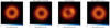 |
Fig. 4 Panels from the first row in Fig. 3, but with a blurring of 20 µas applied. |
| In the text | |
|
Fig. 5 Ground truth image compared to various realizations of directly fitting closure traces for the EHT+ngEHT configuration. Second column: Reconstruction by MOEA/D only fitting closure traces. Third column: Reconstruction by MO-PSO only fitting closure traces. Fourth column: Reconstruction by MO-PSO fitting closure traces and visibilities. |
| In the text | |
|
Fig. 6 Same as Fig. 5, but for the EHT configuration. Additionally, we show in the fifth column a direct reconstruction from the visibilities when leakages at a level of 5% are not corrected. |
| In the text | |
|
Fig. 7 Impact of residual leakage compared to the leakage-independent imaging from the closure traces by MOEA/D. Top row: ground truth image, direct imaging result when leakages are perfectly recovered, and closure trace fitting result from MOEA/D. Middle and bottom row: direct reconstruction results with increasing levels of residual leakage errors (which are not calibrated out of the observation). |
| In the text | |
|
Fig. 8 Ring model (left panel) recovered with MOEA/D and MO-PSO (including polarimetric visibilities) and the 2021 configuration (second and third panel). For comparison, we reprint the reconstruction results in the EHT 2017 array in the last two panels. |
| In the text | |
|
Fig. 9 Reconstructions on real data observed in 2017 by the EHT. Left panel: Reconstruction achieved by directly fitting closure traces with MO-PSO. Right panel: Reconstruction when fitting the Stokes visibilities with DoG-HiT, with the leakage already calibrated. |
| In the text | |
|
Fig. 10 Reconstruction of ALMA Band 6 observations of M87 at 227.1 GHz. |
| In the text | |
|
Fig. A.1 Illustrative sketch of the Pareto front in two dimensions, the construction of the ideal point using the asymptotic behavior along each single axis, and the distance to the Pareto front as a selection criterion. This distance is minimized by MO-PSO. The figure is reprinted from Müller et al. (2023) under CC.BY. 4.0.. |
| In the text | |
|
Fig. D.1 Pareto front of the MOEA/D reconstruction directly fitting to closure traces for the EHT+ngEHT array configuration. The solution in the red box is preferred by MOEA/D as the Pareto-optimal solution closest to the optimum; the cluster with the blue box would have been selected when comparing to closure quantities defined in Thyagarajan et al. (2022) and Samuel et al. (2022). |
| In the text | |
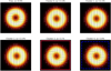 |
Fig. D.2 Same as Fig. D.1, but with a blurring of 20 µas applied to every cluster. |
| In the text | |
|
Fig. D.3 Same as Fig. D.1, but for the EHT array configuration. Additionally, a blurring of 20 µas has been applied to every cluster. |
| In the text | |
|
Fig. D.4 Pareto front of the double source in the EHT+ngEHT configuration. |
| In the text | |
|
Fig. D.5 Pareto front of the SgrA* source model in the EHT+ngEHT configuration. |
| In the text | |
Current usage metrics show cumulative count of Article Views (full-text article views including HTML views, PDF and ePub downloads, according to the available data) and Abstracts Views on Vision4Press platform.
Data correspond to usage on the plateform after 2015. The current usage metrics is available 48-96 hours after online publication and is updated daily on week days.
Initial download of the metrics may take a while.