| Issue |
A&A
Volume 690, October 2024
|
|
|---|---|---|
| Article Number | A224 | |
| Number of page(s) | 16 | |
| Section | Numerical methods and codes | |
| DOI | https://doi.org/10.1051/0004-6361/202450214 | |
| Published online | 11 October 2024 | |
Supervised star, galaxy, and QSO classification with sharpened dimensionality reduction
1
Kapteyn Astronomical Institute, University of Groningen,
Landleven 12,
9747 AD
Groningen,
The Netherlands
2
Netherlands Institute for Radio Astronomy (ASTRON),
Oude Hoogeveensedijk 4,
7991 PD
Dwingeloo,
The Netherlands
3
Bernoulli Institute for Mathematics, Computer Science and Artificial Intelligence, University of Groningen,
Nijenborgh 9,
9747 AG
Groningen,
The Netherlands
4
Department of Information and Computing Sciences, Utrecht University,
Princetonplein 5,
3584 CC
Utrecht,
The Netherlands
★ Corresponding author; martenlourens@gmail.com
Received:
2
April
2024
Accepted:
28
August
2024
Aims. We explored the use of broadband colors to classify stars, galaxies, and quasi-stellar objects (QSOs). Specifically, we applied sharpened dimensionality reduction (SDR)-aided classification to this problem, with the aim of enhancing cluster separation in the projections of high-dimensional data clusters to allow for better classification performance and more informative projections.
Methods. The main objective of this work was to apply SDR to large sets of broadband colors derived from the CPz catalog to obtain projections with clusters of star, galaxy, and QSO data that exhibit a high degree of separation. The SDR method achieves this by combining density-based clustering with conventional dimensionality-reduction techniques. To make SDR scalable and have the ability to project samples using the earlier-computed projection, we used a deep neural network trained to reproduce the SDR projections. Subsequently classification was done by applying a k-nearest neighbors (k-NN) classifier to the sharpened projections.
Results. Based on a qualitative and quantitative analysis of the embeddings produced by SDR, we find that SDR consistently produces accurate projections with a high degree of cluster separation. A number of projection performance metrics are used to evaluate this separation, including the trustworthiness, continuity, Shepard goodness, and distribution consistency metrics. Using the k-NN classifier and consolidating the results of various data sets, we obtain precisions of 99.7%, 98.9%, and 98.5% for classifying stars, galaxies, and QSOs, respectively. Furthermore, we achieve completenesses of 97.8%, 99.3%, and 86.8%, respectively. In addition to classification, we explore the structure of the embeddings produced by SDR by cross-matching with data from Gaia DR3, Galaxy Zoo 1, and a catalog of specific star formation rates, stellar masses, and dust luminosities. We discover that the embeddings reveal astrophysical information, which allows one to understand the structure of the high-dimensional broadband color data in greater detail.
Conclusions. We find that SDR-aided star, galaxy, and QSO classification performs comparably to another unsupervised learning method using hierarchical density-based spatial clustering of applications with noise (HDBSCAN) but offers advantages in terms of scalability and interpretability. Furthermore, it outperforms traditional color selection methods in terms of QSO classification performance. Overall, we demonstrate the potential of SDR-aided classification to provide an accurate and physically insightful classification of astronomical objects based on their broadband colors.
Key words: methods: data analysis / techniques: photometric / surveys / stars: general / galaxies: active / galaxies: general
© The Authors 2024
 Open Access article, published by EDP Sciences, under the terms of the Creative Commons Attribution License (https://creativecommons.org/licenses/by/4.0), which permits unrestricted use, distribution, and reproduction in any medium, provided the original work is properly cited.
This article is published in open access under the Subscribe to Open model. Subscribe to A&A to support open access publication.
1 Introduction
Source detection and classification of celestial objects are key steps in any astronomical analysis. Examples include the classification of stars based on their spectral characteristics, the categorization of galaxy morphologies by following the Hubble sequence (Hubble 1926) and the identification of quasi-stellar objects (QSOs), also known as quasars. In each case, classification requires either high spatial or spectral resolution, which traditionally are expensive in terms of telescope time.
With the advent of multiwavelength surveys, many sophisticated color selection criteria have been developed to isolate stars, galaxies, and active galactic nuclei (AGNs) of which QSOs are a subclass. Simple color-color plots have been extensively used for object classification. For example, Daddi et al. (2004) derived a two-color selection technique using B-, z-, and K-band photometry to isolate star-forming galaxies (SFGs) at z > 1.4 from quiescent galaxies. Similarly, Patel et al. (2012) used a rest-frame U-V versus V-J diagram with galaxies at 0.6 < z < 0.9 to distinguish SFGs from quiescent galaxies. These diagrams are particularly useful at breaking the degeneracy between red quiescent galaxies and reddened SFGs. Additionally, Patel et al. (2012) combined the sample with imaging data from the Hubble Space Telescope (HST) to examine the structure of galaxies in the UVJ diagram. They found that most quiescent galaxies have properties that are characteristic of early-type systems, whereas SFGs display properties of late-type systems. The large spread of SFGs in the UVJ diagram is largely explained by the inclination of each system. Another example of color selection techniques is AGN identification using empirical mid-infrared (MIR) selection criteria. Compared to soft X-ray, ultraviolet (UV; using UV-excess selection, Schmidt & Green 1983), and optical studies, MIR studies are more robust against dust obscuration of AGNs. MIR studies including the works by Stern et al. (2005), Stern et al. (2012), and Assef et al. (2018), using either data from Spitzer or the Wide-field Infrared Survey Explorer (WISE), take advantage of the fact that the MIR spectral energy distribution (SED) of obscured and unobscured AGNs is different from that of normal galaxies. Lastly, to isolate stars from other objects, criteria based on color selection are typically not used. Instead, many surveys use measurements of the extent of objects. An example of this is the star-galaxy separation performed within the Sloan Digital Sky Survey (SDSS) photometric pipeline, which uses the difference between cmodel (i.e., the magnitude obtained from the best-fitting linear combination of the de Vaucouleurs and exponential profiles) and point spread function (PSF) magnitudes to determine whether an object is a star or a galaxy (Lupton et al. 2002).
Currently, sophisticated automated methods are required to extract useful astrophysical information from the ever-increasing volume of extragalactic surveys. As illustrated by Dubath et al. (2017), employing machine-learning methods in the data processing pipelines of such surveys offers a viable solution to a range of problems, including source classification and photometric redshift estimation (see e.g., Carliles et al. 2010). Broadly, there are two different classes of machine-learning methods that can be distinguished by the strategy employed during the training phase. The first is supervised learning, which uses a training set including input features, for example multiwavelength colors, and output labels, such as the class of the astronomical object, to learn the underlying correlations between the input features and output labels. A well-known application of supervised learning is the stellarity parameter in Source Extractor (Bertin & Arnouts 1996, taking inspiration from Odewahn et al. 1992), which uses a neural network trained to determine whether a source is a star based on the extent of sources in astronomical images. Another supervised learning technique is a Bayesian classification technique called kernel discriminant analysis (KDA) or kernel density classification (Richards et al. 2004, 2009), which was used for the photometric selection of UV-excess QSOs from the SDSS. Further applications of supervised learning methods include the use of decision trees (DTs) or support vector machines (SVMs). For example, Ball et al. (2006) demonstrated the use of DTs for star-galaxy classification using data from the SDSS DR3. Vasconcellos et al. (2011) extended upon this by experimenting with various DT algorithms finding that functional trees (FTs) perform best for separating stars and galaxies using photometric data from SDSS DR7. Furthermore, Clarke et al. (2020) used spectroscopically labeled sources from SDSS DR15 to train a random forest (RF) classifier to classify stars, galaxies, and QSOs. Lastly, Kurcz et al. (2016) show how SVMs can be used to classify stars, galaxies, and QSOs using the W1 magnitude and W1 − W2 color from WISE and training using spectral labels from SDSS DR10. The second class of methods is unsupervised learning, which searches for data clusters in the feature space and assigns labels to points based on the clusters to which they belong. A disadvantage of these methods is that they are often unpredictable and harder to understand compared to supervised learning methods, making them difficult to interpret. There exist many different algorithms for unsupervised learning, with varying numbers of hyperparameters, making some harder to tune than others. One such algorithm is HDBSCAN (Campello et al. 2013), hierarchical density-based spatial clustering of applications with noise. This algorithm has been applied by Logan & Fotopoulou (2020, hereafter LF20) to the CPz data set (Fotopoulou & Paltani 2018, hereafter FP18), which consists of a diverse set of stars, galaxies, and QSOs that were selected based on their complete photometric coverage in the optical, near-infrared (NIR), and MIR wavelengths, to perform star, galaxy, and QSO classification. HDBSCAN is an extension of the previous DBSCAN algorithm (Ester et al. 1996), which converts a data set into a hierarchy of connected components based on the distance between objects and defines clusters based on a predefined minimum cluster size. Both algorithms define distances between points as the “mutual reachability distance,” which ensures that sets of sparse and far-away (outlier) points are viewed as being spaced further from higher density regions. This increases the separation between the data and the noise. HDBSCAN extends the DBSCAN algorithm by labeling clusters based on their stability within the hierarchy.
In this paper, we aim to demonstrate that broadband colors can be used to classify stars, galaxies and QSOs through 2D projections of the high-dimensional data. This is not a simple proposition – it is challenging to distinguish data clusters in a 2D projection. To confront this challenge, Kim et al. (2022b) proposed a method called sharpened dimensionality reduction (SDR), which sharpens the high-dimensional data before projecting it via conventional dimensionality reduction (DR) methods. We show that SDR can be used to aid the classification of stars, galaxies and QSOs based on the 2D projections of high-dimensional sets of broadband colors.
The structure of this paper is as follows. Sec. 2 presents the data sets that we use for classification. Sec. 3 introduces various quality metrics that we use to quantify the performance of our projections and classifiers. Sec. 4 discusses the classification model used to perform star, galaxy, and QSO classification. Sec. 5 presents the results of applying our classification on the data sets introduced in Sec. 2. We also look at the various subclusters present in the projection and determine whether they convey meaningful insights by cross-matching with various catalogs. Finally, Sec. 6 compares our results to those obtained through HDBSCAN by LF20 and another classification method based on color selection criteria.
2 Data sets
In this work, we use the CPz catalog for SDR-aided classification, first introduced by FP18 and revised by LF20 to include unsupervised star, galaxy, and QSO classification results from HDBSCAN1. The original purpose of the CPz catalog was to perform classification-aided photometric redshift (z) estimation, hence the abbreviation. The catalog consists of a set of spectroscopically observed sources from different surveys spanning a combined redshift range of z ∈ [0–4] (see Fig. 2a of FP18) with SDSS samples dominating at higher redshifts. The spectroscopic surveys included in CPz are SDSS DR12 (Alam et al. 2015), GAMA DR2 (Liske et al. 2015), VIPERS DR1 (Garilli et al. 2014), VVDS DR2 (Le Fèvre et al. 2013), PRIMUS DR1 (Coil et al. 2011; Cool et al. 2013), and 6dF DR3 (Jones et al. 2004, 2009). The combined sample was filtered by FP18 such that it only included sources of highest spectroscopic redshift quality. Subsequently, FP18 matched the remaining spectroscopic sources to photometric detections by various surveys within an angular radius of 1′. The filters used by each of the photometric surveys cover both the infrared and optical parts of the electromagnetic spectrum. The MIR W1 and W2 filters originate from the WISE ALLWISE data release (Wright et al. 2010; Mainzer et al. 2011; Cutri et al. 2013). The NIR filters, Z, Y, J, H, and Ks, originate from the first cycle of ESO near-IR Public VISTA surveys (Arnaboldi et al. 2007), that is, VIKING (Edge et al. 2013) and VIDEO (Jarvis et al. 2013). The optical u, g, r, i, and z filters originate from SDSS DR12 (Alam et al. 2015), CFHTLS-T0007 Wide (Hudelot et al. 2012), and KiDS DR2 (de Jong et al. 2015).
The CPz catalog consists of total and 3′-aperture apparent magnitudes in the u, g, r, i, z, Y, H, J, and Ks bands and total magnitudes in the W1 and W2 bands. These 20 magnitudes were corrected for Galactic extinction using the Schlegel et al. (1998) maps of Galactic absorption and the Cardelli et al. (1989) extinction law for the Milky Way. Using each of these magnitudes, one can construct a total of 190 unique colors. This is bound to introduce correlations apart from any correlations inherent to the photometric data itself. Generally, machine learning algorithms are very sensitive to the presence of correlations in the input data. Therefore, it is important to remove these correlations as much as possible and end up with a set of most informative colors, a process called feature selection. LF20 attempted to achieve this by constructing multiple RF classifiers for each binary classification problem (i.e., STAR/non-STAR, GAL/non-GAL, and QSO/non-QSO). The resulting RFs were used to obtain a ranked list of colors in order of importance to the classification problem. The top ten of the different color lists are given in Table 2 of LF20. These feature sets still possess significant correlation between different attributes (see Fig. 2 of LF20). This correlation arises because RFs only look at individual attributes at each point in the decision tree, making these classifiers insensitive to correlations between different attributes. Therefore, LF20 decided to combine these lists of important colors with those obtained from the A, B and C RF classifiers in FP18, which were significantly less correlated, to generate numerous attribute sets. A grid search was performed over these sets to find an optimal set for each binary classification problem. The results are listed in Table 3 of LF20. We use the same sets of attributes in this work. For clarity, we list them here in Table 1. When we refer to, for example, the CPzS dataset, which contains stars, galaxies, and QSOs, we are referring to a specific set of colors constructed from the full CPz sample and not to only the objects labeled as stars in the CPz catalog.
Here we apply supervised-learning techniques to train classifiers to label sources based on their location in the projection space provided by the SDR method. Therefore, we require ground-truth class labels to train and validate the performance of these classifiers. The class labels are provided by the CPz catalog used by LF20. The class labels were assigned either automatically, in the case of SDSS spectra, or manually, in the case of VIPERS and VVDS; the other surveys in the CPz catalog do not have labels. A breakdown of the different labels is shown in Table 1 of LF20. In 52% of cases the spectrum had class label UNKNOWN. Therefore, LF20 chose to label these samples as STAR whenever z < 0.0015 and the remaining samples as GAL (i.e., galaxy). Sources labeled as AGN were omitted from the final catalog. After these changes and removals, LF20 ended up with a catalog comprised of in total 48 686 sources of which 7731 were labeled as STAR, 36 763 were labeled as GAL and 4192 were labeled as QSO.
Attributes used for SDR-aided star, galaxy, and QSO classification.
3 Performance metrics
In this section, we discuss several metrics used to evaluate the performance of projection and classification algorithms. We will use such metrics next in Sec. 5 to assess the performance of our proposed joint projection-and-classification pipeline.
3.1 Projection quality metrics
A projection is deemed to be of high quality if it captures well the relationships between high-dimensional data in a low-dimensional (in our case, 2D) space. We use (scalar) quality metrics to quantify the preservation of such relations. We distinguish between three different classes of such metrics, as follows.
The first class of quality metrics are “local neighborhood metrics.” These metrics compare the neighborhoods of samples in both data (i.e., feature) space and projection space and quantify whether various local neighborhood relations are preserved in the projection. The two metrics used in our work are the trustworthiness and continuity metrics.
Trustworthiness (Venna & Kaski 2001) is defined as
![$\[M_{\mathrm{t}}(k)=1-\frac{2}{N k(2 N-3 k-1)} \sum_{i=1}^N \sum_{j \in \mathcal{U}_i^k}(r(i, j)-k),\]$](/articles/aa/full_html/2024/10/aa50214-24/aa50214-24-eq1.png) (1)
(1)
where N is the number of samples in the data set D and k is the number of nearest neighbors to consider2. The set ![$\[\mathcal{U}_i^k\]$](/articles/aa/full_html/2024/10/aa50214-24/aa50214-24-eq2.png) consists of the k nearest neighbors of the sample i in the projection P(D) that are not among the k nearest neighbors of i in the feature space. The quantity r(i, j) specifies the rank of the point j when data vectors are ordered based on their Euclidean distance to a point i in the feature space. All of this ensures that the second term in Eq. (1) quantifies the “proportion of false neighbors” and punishes the metric based on how far these false neighbors are out of the set of nearest neighbors in the feature space (in terms of rank). When the trustworthiness is close to one, the second term in Eq. (1) is close to zero and there are very few false neighbors in the projection. Conversely, when the trustworthiness is close to zero, the second term is close to one and there are many false neighbors in the projection.
consists of the k nearest neighbors of the sample i in the projection P(D) that are not among the k nearest neighbors of i in the feature space. The quantity r(i, j) specifies the rank of the point j when data vectors are ordered based on their Euclidean distance to a point i in the feature space. All of this ensures that the second term in Eq. (1) quantifies the “proportion of false neighbors” and punishes the metric based on how far these false neighbors are out of the set of nearest neighbors in the feature space (in terms of rank). When the trustworthiness is close to one, the second term in Eq. (1) is close to zero and there are very few false neighbors in the projection. Conversely, when the trustworthiness is close to zero, the second term is close to one and there are many false neighbors in the projection.
Continuity is closely related to trustworthiness (Venna & Kaski 2001). Continuity can be computed by swapping D and P(D) in the definition of trustworthiness, that is,
![$\[M_{\mathrm{c}}(k)=1-\frac{2}{N k(2 N-3 k-1)} \sum_{i=1}^N \sum_{j \in \mathcal{V}_i^k}(\hat{r}(i, j)-k),\]$](/articles/aa/full_html/2024/10/aa50214-24/aa50214-24-eq3.png) (2)
(2)
where N and k are as in Eq. (1). The set ![$\[\mathcal{V}_i^k\]$](/articles/aa/full_html/2024/10/aa50214-24/aa50214-24-eq4.png) consists of the k nearest neighbors of the sample i in the feature space that are not among the k nearest neighbors in the projection. The quantity
consists of the k nearest neighbors of the sample i in the feature space that are not among the k nearest neighbors in the projection. The quantity ![$\[\hat{r}(i, j)\]$](/articles/aa/full_html/2024/10/aa50214-24/aa50214-24-eq5.png) specifies the rank of the point j when data vectors are ordered based on their Euclidean distance to a point i in the projection space. Hence the second term in Eq. (2) quantifies the “proportion of missing neighbors” after the projection and penalizes the metric based on how far the missing neighbors are out of the set of nearest neighbors after the projection. When the continuity is close to one, the second term in Eq. (2) is close to zero, meaning there are few missing neighbors in the projection. Conversely, when the continuity is close to zero, the second term in Eq. (2) is close to one, indicating that there are many missing neighbors in the projection. Taken jointly, the Mt and Mc metrics quantify whether local neighborhoods are preserved well in a projection.
specifies the rank of the point j when data vectors are ordered based on their Euclidean distance to a point i in the projection space. Hence the second term in Eq. (2) quantifies the “proportion of missing neighbors” after the projection and penalizes the metric based on how far the missing neighbors are out of the set of nearest neighbors after the projection. When the continuity is close to one, the second term in Eq. (2) is close to zero, meaning there are few missing neighbors in the projection. Conversely, when the continuity is close to zero, the second term in Eq. (2) is close to one, indicating that there are many missing neighbors in the projection. Taken jointly, the Mt and Mc metrics quantify whether local neighborhoods are preserved well in a projection.
The second class of scalar projection performance metrics are “distance preservation metrics.” These metrics quantify the preservation of pointwise distances in the projection space with respect to the data space. In this work, we use the “Shepard goodness” metric, defined as the Spearman rank correlation of the Shepard diagram. The Shepard diagram is a scatter plot showing two measurements of distances between objects, where one distance is the true distance and the other is the distance in some other representation of the objects (Upton & Cook 2014). In our case, these two distances are between points in the feature and projection spaces, respectively. Hence, our Shepard diagram reads (||xi − xj||, ||P(xi) − P(xj)||), with Shepard goodness given by
![$\[M_{\mathrm{S}}=\frac{\operatorname{Cov}~(R(X), R(Y))}{\sigma_{R(X)} \sigma_{R(Y)}},\]$](/articles/aa/full_html/2024/10/aa50214-24/aa50214-24-eq6.png) (3)
(3)
with R(·) denoting the ranking of a vector of samples and X and Y denoting the distances between data in the feature and projection spaces, respectively. The Shepard goodness attains values in the interval [−1, 1], indicating respectively negative and positive correlation between point-wise distances in the data and projection spaces. Negative correlation implies that points close together in the data space are placed far apart in the projection space. Conversely, positive correlation indicates that points close together in the data space are also close together in the projection space. An MS = 0 value indicates no correlation between distances in the data and projection spaces. As for values MS ≤ 0, this tells that the projection is useless in depicting the actual data-space relations.
The last class of scalar projection performance metrics are “class separation metrics.” These metrics quantify the degree of separation between clusters of different class label in the projection space. In our work, we use the distribution consistency and neighborhood hit metrics.
The distribution consistency metric is inspired by the metric introduced by Sips et al. (2009). This metric uses entropy, computed for the distribution of m class labels among the k nearest neighbors of each data point x ∈ D, as a measure of class purity. Let ![$\[n_{c_i}\]$](/articles/aa/full_html/2024/10/aa50214-24/aa50214-24-eq7.png) (x) be the number of data points of class ci in the nearest neighbor set of point x. The Shannon entropy for each data point then reads as
(x) be the number of data points of class ci in the nearest neighbor set of point x. The Shannon entropy for each data point then reads as
![$\[H(\boldsymbol{x}, k)=-\sum_{i=0}^m \frac{n_{c_i}}{\sum_{j=0}^m n_{c_j}} \log _2\left(\frac{n_{c_i}}{\sum_{j=0}^m n_{c_j}}\right).\]$](/articles/aa/full_html/2024/10/aa50214-24/aa50214-24-eq8.png) (4)
(4)
The entropy H is zero when all neighbors have the same class label. Additionally, H = log2(m) when all m classes are mixed equally in a neighborhood. We define the distribution consistency MDC by summing over all data points and normalizing it to zero when all m classes are mixed equally in the neighborhood of each point; and to one when all m classes are well separated in the projection; that is,
![$\[\begin{aligned}M_{\mathrm{DC}}(k) & =1-\frac{1}{N \log _2(m)} \sum_{x \in D} H(\boldsymbol{x}, k) \\& =1+\frac{1}{N \log _2(m)} \sum_{x \in D} \sum_{i=0}^m \frac{n_{c_i}}{\sum_{j=0}^m n_{c_j}} \log _2\left(\frac{n_{c_i}}{\sum_{j=0}^m n_{c_j}}\right).\end{aligned}\]$](/articles/aa/full_html/2024/10/aa50214-24/aa50214-24-eq9.png) (5)
(5)
The neighborhood hit metric is the average over all fractions of k nearest neighbors for each point i that have the same class label as i. Formally it is defined as
![$\[M_{\mathrm{NH}}(k)=\frac{1}{k N} \sum_{i=1}^N\left|\left\{j \in \mathcal{N}_i^k: c_j=c_i\right\}\right|.\]$](/articles/aa/full_html/2024/10/aa50214-24/aa50214-24-eq10.png) (6)
(6)
Here | ·| denotes the cardinality of a set, ![$\[\mathcal{N}_i^k\]$](/articles/aa/full_html/2024/10/aa50214-24/aa50214-24-eq11.png) is the set of nearest neighbors of a point i in the projection space and ci denotes the class label of a point i. A metric value of one implies that data with different labels are well separated.
is the set of nearest neighbors of a point i in the projection space and ci denotes the class label of a point i. A metric value of one implies that data with different labels are well separated.
We note that both of the above cluster separation metrics are only relevant when data are labeled and labels are assigned accurately in line with data clusters present in the high-dimensional space.
In practice, several metrics are jointly used to assess a projection’s quality, since different metrics capture different quality aspects (Nonato & Aupetit 2019; Espadoto et al. 2021). To optimize the SDR parameters of the classification model introduced in Sec. 4 we maximize only the distribution consistency metric. This ensures the projection has the best possible degree of class separation. The other metrics are used to evaluate the preservation of neighborhoods and distances to verify whether we can still draw other conclusions from the projections about the structure of the high-dimensional color space.
3.2 Classification performance metrics
To quantify classification performance, we need to distinguish between binary and multi-label classifiers. Binary classifiers distinguish between two populations, for example, positive and negative, whereas multi-label classifiers distinguish between multiple populations, for example, {star, galaxy, QSO}. For both classifier types, one can construct a confusion matrix from which performance metrics can be derived in a straightforward manner. A confusion matrix represents the counts of predicted vs. actual values. For a binary classifier, the confusion matrix contains true positive (TP), true negative (TN), false positive (FP), and false negative (FN) counts. The metrics derived from such a matrix and used in this work are
Accuracy. The number of correct predictions divided by the total number of predictions, representing the average performance of the classifier over all classes:
![$\[M_{\text {accuracy }}=\frac{\mathrm{TP}+\mathrm{TN}}{\mathrm{TP}+\mathrm{TN}+\mathrm{FP}+\mathrm{FN}};\]$](/articles/aa/full_html/2024/10/aa50214-24/aa50214-24-eq12.png) (7)
(7)
Precision. The number of true positives divided by the total number of elements labeled as belonging to the positive class; also known as “positive predictive power” or, in astronomy, as “purity:”
![$\[M_{\text {precision }}=\frac{\mathrm{TP}}{\mathrm{TP}+\mathrm{FP}}.\]$](/articles/aa/full_html/2024/10/aa50214-24/aa50214-24-eq13.png) (8)
(8)
For a multi-class classifier one can have multiple values for the precision depending on which class is referred to as the “positive” class and which classes are referred to as the “negative” classes;
Recall. The number of true positives divided by the total number of elements that belong to the positive class; also known as “sensitivity,” “hit rate,” “true positive rate,” or, in astronomy, as the “completeness:”
![$\[M_{\text {recall }}=\frac{\mathrm{TP}}{\mathrm{TP}+\mathrm{FN}}.\]$](/articles/aa/full_html/2024/10/aa50214-24/aa50214-24-eq14.png) (9)
(9)
Just as for precision, a multi-class classifier can have multiple values for recall depending on which classes are referred to as “positive” and “negative;” and
F1 score. The harmonic mean of the precision and recall, representing an equal trade-off between the two:
![$\[M_{\mathrm{F} 1}=2 \cdot \frac{M_{\text {precision }} \cdot M_{\text {recall }}}{M_{\text {precision }}+M_{\text {recall }}}.\]$](/articles/aa/full_html/2024/10/aa50214-24/aa50214-24-eq15.png) (10)
(10)
A high precision is important to be confident about the reliability of the classifier, however, this should not come at the cost of losing many of the samples to other classes due to misclassification.
4 Classification model
4.1 Sharpened dimensionality reduction (SDR)
SDR is an integral part of the classification model proposed in this paper. SDR was introduced by Kim et al. (2022b) to tackle the problem of distinguishing high-dimensional data clusters in a 2D projection3. They demonstrate that, for projection techniques that yield poor cluster separation in the 2D space, adding the sharpening step as a preprocessing of the high-dimensional data can enhance the obtained cluster separation.
SDR consists of two separate steps, local gradient clustering (LGC) followed by applying a DR technique of choice, such as one of the well-known techniques Landmark Multidimensional Scaling (LMDS) (De Silva & Tenenbaum 2004; Cox & Cox 2008), t-distributed Stochastic Neighbor Embedding (t-SNE) (van der Maaten & Hinton 2008), and Uniform Manifold Approximation and Projection (UMAP) (McInnes et al. 2018). The goal of LGC is to precondition the high-dimensional data set, allowing the DR method to provide better cluster separation. Note LGC techniques such as described in Fukunaga & Hostetler (1975) and later refined by Comaniciu & Meer (2002) have been used for image segmentation applications and, more recently, the simplification of 2D and 3D trail-sets Hurter et al. (2012); Lhuillier et al. (2017). The key difference to LGC as used in SDR is its application to enhance the density of data having many more dimensions than the usual three present in color images or trail sets.
LGC achieves this density enhancement by iteratively shifting samples along the density gradient in the direction of higher density. Following the procedure introduced by Kim et al. (2022b), the sample density is estimated by constructing a kernel density estimate (KDE) as
![$\[\hat{\rho}\left(x_i\right)=\sum_{x_j \in \mathcal{N}_i^k} \mathcal{K}\left(\frac{\left\|x_i-x_j\right\|}{h_i}\right).\]$](/articles/aa/full_html/2024/10/aa50214-24/aa50214-24-eq16.png) (11)
(11)
In SDR, the choice for 𝒦 is a parabolic, also known as Epanechnikov, kernel (Epanechnikov 1969), which is optimal in a mean-squared error (MSE) sense. The set ![$\[\mathcal{N}_i^k\]$](/articles/aa/full_html/2024/10/aa50214-24/aa50214-24-eq17.png) is the set of k nearest neighbors of a point xi. The parameter hi specifies the bandwidth of the kernel at position xi, set to the distance to the kth-nearest neighbor of xi. This ensures that the KDE is insensitive to the cluster scale. After estimating the local density ρ for xi, the sample can be shifted upward along the normalized density gradient using the update rule
is the set of k nearest neighbors of a point xi. The parameter hi specifies the bandwidth of the kernel at position xi, set to the distance to the kth-nearest neighbor of xi. This ensures that the KDE is insensitive to the cluster scale. After estimating the local density ρ for xi, the sample can be shifted upward along the normalized density gradient using the update rule
![$\[x_i^{\prime}=x_i+\alpha \frac{\nabla \hat{\rho}\left(x_i\right)}{\max \left(\left\|\nabla \hat{\rho}\left(x_i\right)\right\|, \epsilon\right)},\]$](/articles/aa/full_html/2024/10/aa50214-24/aa50214-24-eq18.png) (12)
(12)
where α ≥ 0 is the learning rate and ϵ = 10−5 is a regularization parameter to cater for small gradients. This update rule is applied for a total of T iterations. After each iteration, the KDE defined by Eq. (11) is recomputed.
4.2 SDR-NNP
A major drawback of the SDR technique discussed in Sec. 4.1 is its quite high running time – about 3 hours for a 40K sample, 6-dimensional, dataset. Also, SDR does not have an out-of-sample (OOS) ability. That is, one cannot project a given dataset and, when new data arrives (making the dataset larger), reuse the earlier-computed projection and only focus effort on the new data points. To mitigate these issues, Kim et al. (2022a) introduced sharpened dimensionality reduction with neural network projections (SDR-NNP). This method leverages the scalability, ease-of-use and OOS ability of neural networks by training a deep neural network to reproduce the projection provided by SDR, yielding a method which is three to four orders of magnitude faster than SDR.
Given the above, we use SDR-NNP in our work, based on the deep learning architecture shown in Fig. 1, implemented using TensorFlow (Abadi et al. 2015). It consists of multiple “dense blocks” that halve the number of data dimensions every two layers. The first dense block has dimensions equal to those of the input layer to allow the input data to transform nonlinearly in the high-dimensional data space before projection. The second dense block has a dimensionality that is 3/4 that of the first dense block. Each dense block consists of a dense layer with linear activation, a batch normalization layer, a leaky rectified linear unit (leakyReLU) activation layer, and a dropout layer. The batch normalization layer rescales each batch of data to have zero mean and unit variance. This ensures stability for higher learning rates, making neural network optimization faster (Ioffe & Szegedy 2015). The dropout layer is only active during training and randomly sets input units to zero at a specified “dropout rate.” This prevents the network from overfitting on the training set. The final part of the neural network consists of a dense layer paired with a sigmoid activation layer. The sigmoid activation layer ensures that the coordinates of the 2D projected points generated by the network are normalized between zero and one.
To optimize a neural network we need to specify a loss function λ which quantifies the deviation from the desired result. In our work we use the mean absolute error (MAE)
![$\[\lambda=\frac{1}{2 N} \sum_{i=1}^N\left|x_i-\hat{x}_i\right|+\left|y_i-\hat{y}_i\right|\]$](/articles/aa/full_html/2024/10/aa50214-24/aa50214-24-eq19.png) (13)
(13)
between the ground-truth 2D coordinates (xi, yi) of the N training-set samples provided by the SDR projection and the corresponding 2D coordinates ![$\[\left(\hat{x}_i, \hat{y}_i\right)\]$](/articles/aa/full_html/2024/10/aa50214-24/aa50214-24-eq20.png) inferred by the model. Compared to other typical loss functions such as Mean Square Error (MSE), MAE has shown better optimization results and less sensitivity to outliers in various works that aim to learn DR methods (Espadoto et al. 2020; Modrakowski et al. 2022). We use the Adam optimizer (Kingma & Ba 2014) to find the optimal set of model parameters corresponding to the lowest loss (λ), as Adam performs well for large data sets with a high number of dimensions in the presence of noise and requires little hyperparameter tuning.
inferred by the model. Compared to other typical loss functions such as Mean Square Error (MSE), MAE has shown better optimization results and less sensitivity to outliers in various works that aim to learn DR methods (Espadoto et al. 2020; Modrakowski et al. 2022). We use the Adam optimizer (Kingma & Ba 2014) to find the optimal set of model parameters corresponding to the lowest loss (λ), as Adam performs well for large data sets with a high number of dimensions in the presence of noise and requires little hyperparameter tuning.
 |
Fig. 1 Deep neural network architecture used for SDR-NNP. |
4.3 Classification
The final step of our classification procedure combines the SDR-NNP output with a classifier of choice. We considered four different classifiers: k-nearest neighbors (k-NN), support vector machines (SVM) (Chang & Lin 2011), a multi-layer perceptron (MLPC), and XGBoost (XGBC) (Chen & Guestrin 2016). The k-NN classifier turned out to be the fastest and most easily interpretable of these methods. As such, we use k-NN for the classification presented in this paper.
4.4 Consolidation
We employ three methods to consolidate (combine) the results obtained from the CPzS, CPzG, and CPzq data sets using our k-NN classifier. Namely, lowest entropy consolidation, the alternative method (Logan & Fotopoulou 2020), and the majority vote method, as follows.
Lowest entropy consolidation uses the probability distributions for each sample yielded by the different classifiers to compute the Shannon entropy and selects the classification with the lowest entropy. Additionally, we use an upper limit for the entropy to filter out samples for which none of the considered classifiers yields a good result. These samples are assigned to a post-consolidation “outlier” class.
The alternative and majority vote methods count the occurrence of different class labels. The alternative method assigns any sample for which there is disagreement between the classifiers to the post-consolidation outlier class. The majority vote method is less strict and only assigns samples to the outlier class when the vote is indecisive. In all other cases, samples are assigned to the class with the largest number of votes.
5 Results
5.1 SDR-aided classification
Sec. 4 introduced the classification method we use to classify stars, galaxies and QSOs. Our classification model consists of an SDR-NNP model, which reproduces the projections provided by SDR, and a classifier working in the 2D projection space. We now explain how the SDR method, SDR-NNP model, and classifier are trained and optimized.
Technical set-up. We optimize the SDR parameters with respect to the distribution consistency (MDC) metric by performing a grid search. Since this metric is high when class purity is high (Sec. 3.1), this ensures the projection has the best possible degree of cluster separation, which, in turn, should help our classification. We tested various DR methods including the previously mentioned LMDS, t-SNE, and UMAP, along with Neighborhood Preserving Embedding (NPE) (He et al. 2005), Locally Linear Embedding (LLE) (Roweis & Saul 2000), Laplacian Eigenmaps (Roweis & Saul 2000), Local Tangent Space Alignment (LTSA) (Zhang & Zha 2004), and linear LTSA (Zhang et al. 2007). Of these DR methods, LMDS was one of the best performing in terms of the projection performance metrics introduced in Sec. 3.1. As such, we detail this method next.
Landmark multidimensional scaling (De Silva & Tenenbaum 2004) is an approximation of the classical MDS algorithm (Cox & Cox 2008) which scales well computationally with the sample count N. Landmark multidimensional scaling uses classical MDS to project NL ≪ N “landmark points,” or control points, in the 2D space such that distances between these points are best preserved. Next, LMDS embeds the remaining N − NL points by triangulating their positions with respect to the already placed landmark points. In our work, we considered landmark ratio values NL/N ∈ [0.005, 0.1] with increments of 0.005. Prior to LMDS, we perform a data sharpening step, as described in Sec. 4.1. For the LGC step herein, we tested combinations of α ∈ [0.005, 0.06] with 0.005 increments; k ∈ {25, 75, 125, 175, 225, 275, 325}; and T ∈ {10, 15, 20}.
Projection results. Figure 2a shows the LMDS projection of the CPzS data set having the highest distribution consistency, with MDC ≈ 0.899, over all our tested parameter values. The projection was computed using a subset of 10 000 samples randomly selected from the full projected data set consisting of 48 686 data points. This projection was generated using a landmark ratio of 0.08. In comparison, Fig. 2b shows the sharpened LMDS projection (SLMDS) having an MDC ≈ 0.937, which uses the same landmark ratio as the projection in Fig. 2a. For this projection, we used the values α = 0.03, k = 325, and T = 10.
To better compare the two projections, Table 2 shows the values of all their performance metrics (Sec. 3.1). The values for trustworthiness (MT) and continuity (MC) indicate only a small proportion of false and missing neighbors, so both LMDS and SLMDS preserve local neighborhood relations well. The Shepard goodness values (MS) show that inter-point distances are also well-preserved up to a monotonic scaling relation. The values for the distribution consistency (MDC) and neighborhood hit (MNH) metrics show that SLMDS enhances cluster separation compared to standard LMDS with only a limited decline in MT, MC, and MS. The improvement in cluster separation can also be verified visually by comparing Figs. 2a and 2b. When comparing these graphs, it is important to note that rotation and reflection differences between projections of the same data set can exist. For instance, the blue point cluster appears to the left in the LMDS projection (Fig. 2a and to the right in the SLMDS projection (Fig. 2b). Such variations are irrelevant for the quality of a projection since, as explained in Sec. 3, a good projection aims to preserve the data structure, that is, the relative positions of points with respect to each other, and not their absolute positions within the 2D projection space. It is well known in projection literature that the embedding coordinates (x and y in our case) do not have any particular meaning (Nonato & Aupetit 2019; Coimbra et al. 2016; Broeksema et al. 2013).
Deep learning the projection. Having established that SLMDS improves cluster separation compared to standard LMDS projections, we next train the SDR-NNP model introduced in Sec. 4.2 to mimic the SLMDS projection in Fig. 2b. As explained earlier, this will give us the desired computational scalability and OOS ability. For this process, we used 80% of the data set for training and 20% for testing. The train-test split was performed in a stratified way to preserve the relative fractions of stars, galaxies, and QSOs in both train and test sets.
Figure 3 shows the resulting SDR-NNP projection (top two graphs) and the training history (bottom graph). To find the best set of model parameters, we used 20000 training epochs. We used cross-validation to prevent overfitting at each training epoch, where 25% of the training data were set aside for validation. To check whether our model overfits the training set, we plot the validation loss together with the training loss (Fig. 3 bottom). As visible, there is no increase of the validation loss relative to the training loss, and therefore there is no overfitting. Furthermore, we plot separately the training loss and inferential training loss, because the batch normalization layers in the neural network behave differently during training and inference. As visible from Fig. 3 bottom, these two values are nearly identical over the training period. Finally, we compare the final training loss (computed at the end of the 20K training epochs) with the test loss. The final training loss (rightmost point in the bottom graph in Fig. 3) is equal to 0.0099. The test loss has a value of 0.0101. These values are close, implying that the trained neural network generalizes well to unseen data.
Comparing the SDR and SDR-NNP embeddings in Fig. 3, we see that SDR-NNP removes much of the segmentation present in the SDR embedding, making the projection appear more continuous – that is, the black, blue, and orange points appear less separated into small “islands” in SDR-NNP as compared to SDR. However, these plots show that SDR-NNP keeps the essence of the data separation we are after, namely that the star (black), galaxy (yellow), and QSO (blue) clusters appear separated from each other. As we shall see next, this is precisely the separation we need for classification.
Classification. As mentioned in Sect. 4.3, we have considered four different classifiers. We next focus on the results for the k-NN classifier, which, as explained in Sect. 4.3, yielded the best results from four tested classifiers. In the following, we again used a stratified train-test split where 80% of the data were used for training the classifier and 20% were used for testing, respectively.
Figure 4 shows the k-NN classification results for projections of the CPzS, CPzG, and CPzQ data sets generated through SDR-NNP trained on their corresponding SLMDS projections. The left plots show the respective SDR-NNP projections (scatter plots) atop of the decision maps generated by k-NN. That is, all data points which project in a 2D area (decision zone) having a given color will be assigned the label corresponding to that color by the classifier. Since we use a k-NN classifier in the 2D projection space, the decision zones are roughly equivalent to Voronoi diagrams of the respective three sets of labels (STAR, GAL, and QSO). Neighbor pixels in these 2D maps which have different colors indicate decision boundaries, that is, locations where the k-NN classifier changes the inferred label. We note that more general (but more complex) methods exist for computing and visualizing decision maps (Wang et al. 2023; Rodrigues et al. 2019). However, in our case, we do not need to use such methods, since our classifier directly works on the 2D, rather than the high-dimensional, data space. The images in the right column of Fig. 4 show the confusion matrices for the respective three classifiers.
The results in Fig. 4 show that k-NN is able to generate both accurate and precise simultaneous classifications of stars, galaxies and QSOs based on the SLMDS-NNP projections of the various data sets. The highest accuracies of 97.9% are achieved using the classifiers based on the CPzG and CPzQ data sets. Furthermore, each of the trained models classifies stars with near one hundred percent precision, and galaxies with 98% precision, respectively. The most challenging class to classify is the QSO class, for which we achieve a maximum precision of 94% by the classifier trained using the CPzG data set. Additionally, the QSO class also has the lowest completeness (or recall).
Consolidated results. To boost performance for QSO classification, we consolidate the results yielded by the three SLMDS-NNP based k-NN classifiers, following the three consolidation methods introduced in Sec. 4.4.
Table 3 shows the results. The star and galaxy classification performance is similar to that yielded by the three individual classifiers, but there is an improvement in terms of QSO classification performance. We also see that the lowest-entropy consolidation method yields the lowest completeness for the galaxy and QSO classes, mainly due to the large number of outliers selected by this method. This is due to the chosen post-consolidation entropy threshold of 0.1.
The outliers selected by each of the consolidation methods lie mostly along the decision boundaries shown in Fig. 4. Graphs demonstrating this are not included in this article for space reasons. The post-consolidation outlier class of the lowest entropy method contains 26 stars, 427 galaxies and 246 QSOs. The large number of galaxies is unsurprising, since 76% of the full data set consists of galaxies; on the other hand, QSOs only constitute 9% of the full data set. Part of this can be explained by the way star and galaxy labels were assigned. As explained in LF20, 52% of the CPz sample had class label “UNKNOWN.” Therefore, they decided to assign labels to these samples according to the spectroscopic redshift of each object. Samples with a redshift less than 0.0015 were assigned to the star class, while samples with a higher redshift were assigned to the galaxy class. This can cause QSOs to have been mistakenly labeled as galaxies, explaining the relatively high number of post-consolidation outliers. Additionally, in the rare cases where galaxies are moving toward us or away from us with a velocity less than 450 km s−1, galaxies can become mislabeled as stars.
The classification performance metrics in Table 3 clearly show that, while the lowest entropy consolidation results have lower values for accuracy and recall, we achieve a higher precision for the QSO class compared to not using consolidation. The higher precision is due to the entropy threshold, which ensures fewer sources are misclassified by assigning them to the outlier class. The alternative method is the second-best performing method in terms of precision whilst retaining a high completeness. With a precision of 95.6%, the alternative method shows a marginal improvement over the individual SLMDS-NNP based k-NN classifiers. Finally, the majority vote method forms the best trade-off between precision and completeness for QSO classification, as evident from its F1 score (MF1).
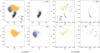 |
Fig. 2 Comparison between LMDS and SLMDS projections. Panels (a) the LMDS projection (MDC ≈ 0.899) and (b) SLMDS projection (MDC ≈ 0.937 with α = 0.03, k = 325, and T = 10), for the CPzS data set. All plots use a landmark ratio of 0.08. Samples are colored by the labels provided by the CPz catalog. |
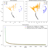 |
Fig. 3 SDR-NNP results for the CPzs data set. Top left: SDR embedding of the test set using 20% of the full data set. Top right: corresponding SDR-NNP embedding. Bottom: training loss, validation loss and inferential training loss as a function of training effort (epochs). |
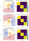 |
Fig. 4 Decision boundaries and confusion matrices for the SDR-aided classifiers trained on each of the three datasets presented in Table 1. Left: decision boundaries of a k-NN classifier trained on the projection obtained by SDR-NNP for the CPzS (4a), CPzG (4b), and CPzQ (4c) data sets. Right: confusion matrices for the three classifiers. |
Post-consolidation performance of classification.
5.2 Physical interpretation of subclusters in SDR projections
Many SDR projections contain subclusters, for example, the SLMDS projection shown in Fig. 2b. To determine whether these subclusters convey any relevant information and to unravel the overall structure of the SDR projections, we can cross-match the objects in these subclusters with existing astronomical catalogs. This process is akin to the way many of the traditional color selection criteria in astronomy were developed; see for example Daddi et al. (2004) and Patel et al. (2012).
Stellar subclusters. We first consider the subclusters present in the stellar sample of the SLMDS projection of the CPzS data set. To determine whether these subclusters are physical clumps or result from an artificial oversegmentation of the projection (due to SDR’s LGC step, see Sec. 4.1), we cross-match them with the astrophysical parameters data set of Gaia DR3 (Gaia Collaboration 2016, 2023), generated from Gaia data using the GSP-Phot module in the Apsis (Astrophysical parameters inference system) pipeline (Creevey et al. 2023). These parameters allow us to plot Hertzsprung-Russell (HR) and surface gravity-effective temperature diagrams, shown in Fig. 5. The vertical branch around 6000 K in both of these plots is the giant branch. We observe that the subclusters not only convey temperature information but also the spectral type of the stars, by noticing a shift in effective temperature of stars within the same subcluster as we move up in magnitude and down in surface gravity. In addition, since LMDS is a distance-preserving DR technique, we infer from Figs. 5 and 2b that stars with a low effective temperature (in blue), which roughly coincide with the M spectral class, have colors that most closely match those of galaxies. The HR and surface gravity-effective temperature diagrams both show that the sharpening step of SDR has oversegmented the stellar data, since the sequences in both of these diagrams are continuous. However, this exercise demonstrates that the projection still retains important astrophysical information, even if it is (perhaps unnecessarily) oversegmented.
Galaxy subclusters. We now examine the structure of the galaxy sample in the SLMDS projection of the CPzS data set. We cross-match with the Galaxy Zoo 1 (GZ1) data release (Lintott et al. 2008, 2011) and a catalog of stellar masses and star formation rates from Chang et al. (2015). The former allows us to determine whether there is a clear separation between early and late-type galaxies in the projection similar to that found by Patel et al. (2012) in the UV J diagram. The latter data set allows us to investigate whether there is a clear distinction between SFGs and quiescent galaxies.
The GZ1 data contains morphological classifications of nearly 900000 galaxies from SDSS DR6 and 7 (Adelman-McCarthy et al. 2008; Abazajian et al. 2009), classified by hundreds of thousands of volunteers. The task of each volunteer was to assign each object to one of six categories. The categories are elliptical (which likely also includes lenticular, that is, S0, galaxies), clockwise spiral galaxies, anti-clockwise spiral galaxies, some other kind of spiral galaxy (for example edge-on), star or unknown, and merger. The votes for each object were subsequently combined into fractions which can be used for further study. Lintott et al. (2011) used the techniques described by Bamford et al. (2009) to remove the bias introduced by the survey limits of SDSS. The survey limits can cause small, faint or distant galaxies to be misclassified as elliptical galaxies due to spiral arms not being visible in SDSS images. To alleviate this effect, Bamford et al. (2009) devised a technique to estimate this bias and correct for it by assuming the morphological fraction within bins of fixed galaxy size and luminosity to be constant in redshift. Since redshift is a required parameter for this technique, objects needed to be spectroscopically observed by SDSS. Lintott et al. (2011) supplemented the redshifts provided by SDSS DR6 with those provided by DR7 which meant that 92% of the objects in the main galaxy sample of GZ1 had spectroscopic redshifts. Furthermore, the debiasing procedure requires a homogeneous distribution of a substantial number of galaxies, that is, at least 30, to be present in each bin in the size versus absolute magnitude space at low redshifts. This limits the debiasing procedure to objects with reliable r-band magnitudes, sizes that are not outliers from the normal galaxy distribution and redshifts between 0.001 and 0.25. The debiasing technique used by Lintott et al. (2011) resulted in a set of three debiased fractions: the debiased fractions of objects assigned to any of the spiral (psp), elliptical (pel) and otherwise (i.e., star, merger, or unknown) (px) categories.
We find a total of 15 412 matches with GZ1, of which 13 467 have spectroscopic redshifts between 0.001 and 0.25. The debiased fractions for each sample in the SLMDS projection of the CPzS data set are shown in Fig. 6. To check the validity of the debiased vote fractions, we also include a plot showing the redshifts of the various objects. From these plots we infer that there is no clear indication that many of the subclusters within the galaxy class produced by SDR convey anything meaningful about the morphological type of the galaxies. However, there seems to be a separation between late-type (i.e., spiral) and early-type (i.e., elliptical) galaxies toward the top left corner of the SLMDS projection. Analogous to traditional color selection, one can develop selection criteria to classify these samples as spiral galaxies. Alternatively, one can apply clustering algorithms. However, the lack of OOS support of SDR and the stochastic nature of LMDS make these methods impractical for large-scale classification and irreproducible. To mitigate this issue, we need an SDR-NNP model that is able to reproduce the galaxy subclusters in the SDR embedding.
Furthermore, we note that there appears to be a redshift gradient in the top left plot of Fig. 6. This gradient is likely caused by the fact that the CPzS data set contains colors constructed using apparent magnitudes as opposed to rest frame magnitudes. This causes the same set of colors to probe different parts of a galaxy’s spectrum when galaxies are located at different redshifts. Further exploration using rest frame colors might uncover other underlying causes for the spread in the main galaxy cluster but that is left for future work.
In addition to inspecting the morphologies of galaxies, we also examine the specific star-formation rate (sSFR) (i.e., the SFR per unit stellar mass of the galaxy), stellar mass, and dust luminosity of the galaxies in the CPzS data set. These parameters were obtained by cross-matching with a catalog produced by Chang et al. (2015) by fitting SEDs to the optical and MIR spectra obtained by SDSS and WISE and are used to color-code the projected galaxy data in Fig. 7. We find a total of 14 670 matches.
We observe a gradient in stellar mass similar to the redshift gradient observed in the top left panel of Fig. 6. This can be due to the selection functions of the various surveys included in the CPz catalog which can cause low-mass galaxies to be underrepresented at higher redshifts. The dust luminosity (bottom panel of Fig. 7) also shows a slight gradient in this projection, with galaxies with a low dust luminosity being closer to the stellar sample in the SDR projection. We do not find a coherent structure in the distribution of sSFR in the projection (top panel of Fig. 7).
Comparing Figs. 5 and 6, we notice that the colors of elliptical galaxies most closely resemble M stars in the CPz catalog. This observation is motivated by the fact that LMDS is a distance preserving DR method, implying that the 2D projection should preserve distances between the color coordinates in the high-dimensional space. Coupled with the sharpening step, we have shown that SLMDS still preserves distances reasonably well – see the value of the Shepard goodness metric in Table 2. Most of the galaxies in the subcluster closest to the M-star subcluster in Fig. 5 are ellipticals with a redshift ~0.08. Furthermore, they have sSFR < 10−11 yr−1, that is, they are quiescent. Additionally, they have stellar masses 1010−1011 M⊙, typical of elliptical galaxies and relatively low dust luminosities of ~109 L⊙. These properties suggest that these galaxies are best represented by an old stellar population with little dust obscuration in the NIR.
Examining Table 1, we note that many of the colors in the CPzS data set are comprised of NIR broadband magnitudes. Therefore, the projection likely reflects mostly NIR color relations. From Fig. 14 in Verro et al. (2022), which provides the contribution of red giant branch (RGB) stars and thermally pulsing asymptotic giant branch (TP-AGB) stars to the K-band luminosity in various single stellar population (SSP) models using the X-shooter Spectral Library, we see that, for old stellar populations with ages ≳ 2 Gyr, the K-band luminosity is mostly dominated by RGB stars, which are K and M giants. This might explain why these elliptical galaxies closely resemble M stars in terms of their NIR colors and why they are placed closely together in the SLMDS projection.
QSO subclusters. Finally, we examine the redshift distribution of the QSO sample in the SLMDS projection of the CPzS data set. Figure 8 shows this projection with the redshifts color coded. We observe a redshift gradient similar to the one observed for the main galaxy sample in the top left panel of Fig. 6 with most low-redshift QSOs (z ≤ 1) overlapping with the galaxy cluster. In analogy to the galaxies, this gradient is likely caused by the set of colors probing different parts of the QSO’s spectral energy distribution (SED).
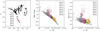 |
Fig. 5 Analysis of the subclusters present in the SLMDS projection using astrophysical parameters from Gaia DR3 (Gaia Collaboration 2023; Creevey et al. 2023). Left: SLMDS projection of the CPzS data set with selected subclusters, each marked by an individual color. HR (middle) and surface gravity (log g) versus effective temperature (Teff) (right) diagrams. In these two plots, points are colored by their cluster, as given by the SDR projection. |
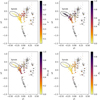 |
Fig. 6 CPzS data set projected using SLMDS cross-matched with the GZ1 classifications. The top left plot shows the redshift of the galaxies in GZ1. The classifications (i.e., top right, bottom left, and bottom right plots) are color coded by the debiased vote fractions of the spiral (psp), elliptical (pel), and otherwise (i.e., star, merger, or unknown) (px) categories following from the debiasing technique of Bamford et al. (2009). For reliable debiasing of the classifications, the redshift should be in the range 0.001–0.25 (Lintott et al. 2011). |
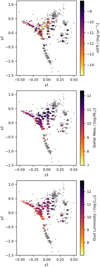 |
Fig. 7 CPzS data set projected using SLMDS cross-matched with a catalog of sSFRs (top), stellar masses (middle), and dust luminosities (bottom) of various galaxies composed by Chang et al. (2015). |
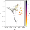 |
Fig. 8 CPzS data set projected using SLMDS with the redshifts of the various QSOs color coded. |
6 Summary and conclusions
In this paper we aimed to answer the question whether broadband colors can be used to accurately and simultaneously classify stars, galaxies and QSOs; specifically, we looked at the added value of dimensionality reduction (DR) methods as tools to assist the aforementioned classification process. For this, we proposed to precondition the high-dimensional data, consisting of broadband colors, to sharpen the high-dimensional data clusters, to increase the corresponding separation between clusters in a 2D projection constructed with DR methods. For this, we used SDR, which improves the cluster separation of the well-known LMDS projection method, and SDR-NNP, which improves the computational performance and adds OOS ability to the SDR method. We next showed that such an enhanced 2D separation can be obtained and, importantly for our goal, this separation helps training relatively simple classifiers (k-NN) in the 2D projection space to achieve highly accurate results in terms of labeling stars, galaxies, and QSOs.
We considered three data sets, the CPzS, CPzG, and CPzQ, constructed from the CPz catalog, which contains data from several surveys. The CPz catalog was introduced by Fotopoulou & Paltani (2018) and later revised by Logan & Fotopoulou (2020). Each of the data sets are composed of unique sets of colors (Table 1), which lie mainly in the NIR, and are optimized for the three binary classification problems, that is, star/non-star, galaxy/non-galaxy, and QSO/non-QSO.
Our results show that SDR (and SDR-NNP) can be used to consistently produce projections with a high degree of cluster separation between stars, galaxies, and QSO clusters – see Fig. 4.
To quantitatively evaluate the degree of cluster separation, we used two cluster separation metrics – distribution consistency and neighborhood hit. To further evaluate how well our projections preserve the data structure – and thus if we can use such projections to extract reliable astrophysical information – we examined the projections’ neighborhood and distance preservation metrics. Results for trustworthiness and continuity show that, while the SDR sharpening step changes the structure of the high-dimensional data, neighborhood relations are still well-preserved. Furthermore, the Shepard goodness, a distance-preservation metric, shows that global distances are also well-preserved by SDR (up to a monotonic scaling). We next investigated the structure of the projection of the CPzS data set generated using sharpened LMDS and find that we can unravel structures present in it and obtain results similar to those derived from color-color diagrams.
To further address two key limitations of the SDR projection method – its lack of out-of-sample (OOS) ability, which makes its results stochastic; and its low computational scalability – we used deep learning to emulate the projections produced using SDR. Our methods also allow one to experiment with the embeddings, for example, applying SDR-NNP to k-corrected galactic colors to determine whether the main galaxy cluster indeed becomes more compact (see Sec. 5). On the positive side, SDR-NNP is simple to construct, easy to train, and yields good cluster separation between the star, galaxy, and QSO samples, so that one can use the resulting 2D projections to construct high-quality classifiers for stars, galaxies, and QSO samples with minimal effort. On the negative side, SDR-NNP fails to fully reproduce the precise segmentation within the star, galaxy, and QSO samples. From the training history plotted in Fig. 3, we see that, to preserve such fine-structure, larger and/or more complex neural networks are needed. We reserve the exploration of such neural networks for future work.
In this work we mainly focus on three data sets mostly composed of different NIR broadband colors, all derived from the CPz catalog. Future work is needed to examine how SDR-aided classification performs on different data sets containing, for example, only optical broadband colors. In addition, one may be justified to investigate how SDR-aided classification can be applied to individual large astronomical surveys, which usually only have a smaller set of filters over a more limited wavelength range.
To classify stars, galaxies and QSOs, we proposed a novel approach that uses only the information present in the 2D projection space. We showed that, due to the high separation produced by SDR in data space, a relatively simple classifier, k-NN, can already yield very good performance using only this 2D space, as tested on the CPzS, CPzG, and CPzQ data sets. To improve QSO classification performance, we consolidated the results using three consolidation methods. We achieve the highest precision for the QSO class using the lowest entropy consolidation method, with 99.7%, 98.9%, and 98.5% precision for classifying stars, galaxies, and QSOs, respectively. In comparison, Logan & Fotopoulou (2020) achieve a respective precision of 99.6%, 98.4% and 94.9% using HDBSCAN and the alternative consolidation method. Separately, Stern et al. (2012) were able to identify Spitzer MIR AGN candidates with 95% precision using a simple criterion based on NIR colors developed using WISE data. We achieve the highest completeness for the QSO class using the majority vote consolidation method, with 97.5%, 99.3%, and 86.8% completeness for classifying stars, galaxies, and QSOs, respectively. In comparison, Logan & Fotopoulou (2020) achieve completenesses of 97.8%, 99.0%, and 88.1%, respectively, using highest-probability consolidation, while Stern et al. (2012) obtained a MIR AGN completeness of only 78%.
Summarizing the above, our SDR-aided star, galaxy, and QSO classification method produces results on a par with, or even (slightly) exceeding, the results obtained using HDB-SCAN by Logan & Fotopoulou (2020) in terms of precision and completeness. Furthermore, our method outperforms traditional color selection techniques such as presented by Stern et al. (2012) in terms of precision and completeness whilst retaining interpretability. Compared to HDBSCAN, SDR-aided classification has a number of advantages. Firstly, it has OOS ability through the use of SDR-NNP models. This ability makes it more scalable than HDBSCAN, which needs to be rerun every time new data becomes available. Additionally, one can apply SDR on a small representative subset of the full data set and then train an SDR-NNP model to project the rest of the data. Moreover, SDR-aided classification is less of a “black-box,” as it is a supervised-learning method. This allows the user to inspect the decision boundaries in the projections and determine whether the classification works properly. We have also demonstrated that one can validate whether SDR projections are accurate by computing various projection performance metrics. Finally, we have shown that our SDR-aided classification can be interpreted to reveal astrophysical properties of the classified objects, something that appears difficult with HDBSCAN. An example of another application of SDR-aided classification allowing for astrophysical interpretation is the analysis of GALAH+ DR3 (Buder et al. 2021) and Gaia DR3 (Gaia Collaboration 2023) data to understand the formation of the Milky Way’s halo (Kim 2023).
The code developed for this research is written in Python and consists of two modules. The first module, called “pySDR,” wraps the code developed by Kim et al. (2022b) to apply Sharpened Dimensionality Reduction in Python. The second module, named “SHARC” (SHArpened Dimensionality Reduction & Classification), is used to apply all the analysis presented in this paper. This includes computing performance metrics, SDR optimization, training a neural network to apply SDR, performing classification, and consolidating classification results4.
Acknowledgements
The authors would like to thank S. Fotopoulou for discussions that led to the genesis of this work. We would also like to thank the referee for suggestions that helped improve the clarity of the text and put the work in a better context. Y. Kim’s work was partially supported by the DSSC Doctoral Training Programme co-funded by the Marie Sklodowska-Curie COFUND project (DSSC 754315). Funding for the SDSS and SDSS-II has been provided by the Alfred P. Sloan Foundation, the Participating Institutions, the National Science Foundation, the U.S. Department of Energy, the National Aeronautics and Space Administration, the Japanese Monbukagakusho, the Max Planck Society, and the Higher Education Funding Council for England. The SDSS Web Site is http://www.sdss.org/. The SDSS is managed by the Astrophysical Research Consortium for the Participating Institutions. The Participating Institutions are the American Museum of Natural History, Astrophysical Institute Potsdam, University of Basel, University of Cambridge, Case Western Reserve University, University of Chicago, Drexel University, Fermilab, the Institute for Advanced Study, the Japan Participation Group, Johns Hopkins University, the Joint Institute for Nuclear Astrophysics, the Kavli Institute for Particle Astrophysics and Cosmology, the Korean Scientist Group, the Chinese Academy of Sciences (LAMOST), Los Alamos National Laboratory, the Max-Planck-Institute for Astronomy (MPIA), the Max-Planck-Institute for Astrophysics (MPA), New Mexico State University, Ohio State University, University of Pittsburgh, University of Portsmouth, Princeton University, the United States Naval Observatory, and the University of Washington. Funding for SDSS-III has been provided by the Alfred P. Sloan Foundation, the Participating Institutions, the National Science Foundation, and the U.S. Department of Energy Office of Science. The SDSS-III web site is http://www.sdss3.org/. SDSS-III is managed by the Astrophysical Research Consortium for the Participating Institutions of the SDSS-III Collaboration including the University of Arizona, the Brazilian Participation Group, Brookhaven National Laboratory, Carnegie Mellon University, University of Florida, the French Participation Group, the German Participation Group, Harvard University, the Instituto de Astrofisica de Canarias, the Michigan State/Notre Dame/JINA Participation Group, Johns Hopkins University, Lawrence Berkeley National Laboratory, Max Planck Institute for Astrophysics, Max Planck Institute for Extraterrestrial Physics, New Mexico State University, New York University, Ohio State University, Pennsylvania State University, University of Portsmouth, Princeton University, the Spanish Participation Group, University of Tokyo, University of Utah, Vanderbilt University, University of Virginia, University of Washington, and Yale University. GAMA is a joint European-Australasian project based around a spectroscopic campaign using the Anglo-Australian Telescope. The GAMA input catalogue is based on data taken from the Sloan Digital Sky Survey and the UKIRT Infrared Deep Sky Survey. Complementary imaging of the GAMA regions is being obtained by a number of independent survey programmes including GALEX MIS, VST KiDS, VISTA VIKING, WISE, Herschel-ATLAS, GMRT and ASKAP providing UV to radio coverage. GAMA is funded by the STFC (UK), the ARC (Australia), the AAO, and the participating institutions. The GAMA website is http://www.gama-survey.org/. This paper uses data from the VIMOS Public Extragalactic Redshift Survey (VIPERS). VIPERS has been performed using the ESO Very Large Telescope, under the “Large Programme” 182.A-0886. The participating institutions and funding agencies are listed at http://vipers.inaf.it. This research uses data from the VIMOS VLT Deep Survey, obtained from the VVDS database operated by Cesam, Laboratoire d’Astrophysique de Marseille, France. Funding for PRIMUS is provided by NSF (AST-0607701, AST-0908246, AST-0908442, AST-0908354) and NASA (Spitzer-1356708, 08-ADP08-0019, NNX09AC95G). This publication makes use of data products from the Wide-field Infrared Survey Explorer, which is a joint project of the University of California, Los Angeles, and the Jet Propulsion Laboratory/California Institute of Technology, funded by the National Aeronautics and Space Administration. Based on observations collected at the European Southern Observatory under ESO programmes 179.A-2004 and 179.A-2006. Based on observations obtained with MegaPrime/MegaCam, a joint project of CFHT and CEA/IRFU, at the Canada-France-Hawaii Telescope (CFHT) which is operated by the National Research Council (NRC) of Canada, the Institut National des Science de l’Univers of the Centre National de la Recherche Scientifique (CNRS) of France, and the University of Hawaii. This work is based in part on data products produced at Terapix available at the Canadian Astronomy Data Centre as part of the Canada-France-Hawaii Telescope Legacy Survey, a collaborative project of NRC and CNRS. Based on data products from observations made with ESO Telescopes at the La Silla Paranal Observatory under programme IDs 177.A-3016, 177.A-3017 and 177.A-3018, and on data products produced by Target/OmegaCEN, INAF-OACN, INAF-OAPD and the KiDS production team, on behalf of the KiDS consortium. OmegaCEN and the KiDS production team acknowledge support by NOVA and NWO-M grants. Members of INAF-OAPD and INAF-OACN also acknowledge the support from the Department of Physics & Astronomy of the University of Padova, and of the Department of Physics of Univ. Federico II (Naples). This work has made use of data from the European Space Agency (ESA) mission Gaia (https://www.cosmos.esa.int/gaia), processed by the Gaia Data Processing and Analysis Consortium (DPAC, https://www.cosmos.esa.int/web/gaia/dpac/consortium). Funding for the DPAC has been provided by national institutions, in particular the institutions participating in the Gaia Multilateral Agreement. This research has made use of the VizieR catalogue access tool, CDS, Strasbourg, France.
References
- Abadi, M., Agarwal, A., Barham, P., et al. 2015, TensorFlow: Large-Scale Machine Learning on Heterogeneous Systems, software available from tensorflow.org [Google Scholar]
- Abazajian, K. N., Adelman-McCarthy, J. K., Agüeros, M. A., et al. 2009, ApJS, 182, 543 [Google Scholar]
- Adelman-McCarthy, J. K., Agüeros, M. A., Allam, S. S., et al. 2008, ApJS, 175, 297 [NASA ADS] [CrossRef] [Google Scholar]
- Alam, S., Albareti, F. D., Allende Prieto, C., et al. 2015, ApJS, 219, 12 [Google Scholar]
- Arnaboldi, M., Neeser, M. J., Parker, L. C., et al. 2007, The Messenger, 127, 28 [NASA ADS] [Google Scholar]
- Assef, R. J., Stern, D., Noirot, G., et al. 2018, ApJS, 234, 23 [Google Scholar]
- Ball, N. M., Brunner, R. J., Myers, A. D., & Tcheng, D. 2006, ApJ, 650, 497 [NASA ADS] [CrossRef] [Google Scholar]
- Bamford, S. P., Nichol, R. C., Baldry, I. K., et al. 2009, MNRAS, 393, 1324 [NASA ADS] [CrossRef] [Google Scholar]
- Bertin, E., & Arnouts, S. 1996, A&AS, 117, 393 [NASA ADS] [CrossRef] [EDP Sciences] [Google Scholar]
- Broeksema, B., Telea, A. C., & Baudel, T. 2013, Comput. Graph. Forum, 32, 158 [CrossRef] [Google Scholar]
- Buder, S., Sharma, S., Kos, J., et al. 2021, MNRAS, 506, 150 [NASA ADS] [CrossRef] [Google Scholar]
- Campello, R. J. G. B., Moulavi, D., & Sander, J. 2013, in Advances in Knowledge Discovery and Data Mining, eds. J. Pei, V. S. Tseng, L. Cao, H. Motoda, & G. Xu (Berlin, Heidelberg: Springer), 160 [Google Scholar]
- Cardelli, J. A., Clayton, G. C., & Mathis, J. S. 1989, ApJ, 345, 245 [Google Scholar]
- Carliles, S., Budavári, T., Heinis, S., Priebe, C., & Szalay, A. S. 2010, ApJ, 712, 511 [NASA ADS] [CrossRef] [Google Scholar]
- Chang, C.-C., & Lin, C.-J. 2011, ACM Trans. Intell. Syst. Technol., 2, 27 [CrossRef] [Google Scholar]
- Chang, Y.-Y., van der Wel, A., da Cunha, E., & Rix, H.-W. 2015, ApJS, 219, 8 [Google Scholar]
- Chen, T., & Guestrin, C. 2016, in Proceedings of the 22nd ACM SIGKDD International Conference on Knowledge Discovery and Data Mining, KDD’16 (New York, NY, USA: ACM), 785 [CrossRef] [Google Scholar]
- Clarke, A. O., Scaife, A. M. M., Greenhalgh, R., & Griguta, V. 2020, A&A, 639, A84 [NASA ADS] [CrossRef] [EDP Sciences] [Google Scholar]
- Coil, A. L., Blanton, M. R., Burles, S. M., et al. 2011, ApJ, 741, 8 [Google Scholar]
- Coimbra, D. B., Martins, R. M., Neves, T. T., Telea, A. C., & Paulovich, F. V. 2016, Inform. Visual., 15, 154 [Google Scholar]
- Comaniciu, D., & Meer, P. 2002, IEEE Trans. Pattern Anal. Mach. Intell., 24, 603 [CrossRef] [Google Scholar]
- Cool, R. J., Moustakas, J., Blanton, M. R., et al. 2013, ApJ, 767, 118 [NASA ADS] [CrossRef] [Google Scholar]
- Cox, M. A. A., & Cox, T. F. 2008, Multidimensional Scaling (Berlin, Heidelberg: Springer), 315 [Google Scholar]
- Creevey, O. L., Sordo, R., Pailler, F., et al. 2023, A&A, 674, A26 [NASA ADS] [CrossRef] [EDP Sciences] [Google Scholar]
- Cutri, R. M., Wright, E. L., Conrow, T., et al. 2013, Explanatory Supplement to the AllWISE Data Release Products [Google Scholar]
- Daddi, E., Cimatti, A., Renzini, A., et al. 2004, ApJ, 617, 746 [NASA ADS] [CrossRef] [Google Scholar]
- de Jong, J. T. A., Verdoes Kleijn, G. A., Boxhoorn, D. R., et al. 2015, A&A, 582, A62 [NASA ADS] [CrossRef] [EDP Sciences] [Google Scholar]
- De Silva, V., & Tenenbaum, J. B. 2004, Sparse multidimensional scaling using landmark points, Tech. rep., Stanford University [Google Scholar]
- Dubath, P., Apostolakos, N., Bonchi, A., et al. 2017, in Astroinformatics, 325, eds. M. Brescia, S. G. Djorgovski, E. D. Feigelson, G. Longo, & S. Cavuoti, 73 [Google Scholar]
- Edge, A., Sutherland, W., Kuijken, K., et al. 2013, The Messenger, 154, 32 [NASA ADS] [Google Scholar]
- Epanechnikov, V. A. 1969, Theory Probab. Appl., 14, 153 [Google Scholar]
- Espadoto., M. Hirata., N. S. T., Falcão., A. X., & Telea., A. C. 2020, in Proceedings of the 15th International Joint Conference on Computer Vision, Imaging and Computer Graphics Theory and Applications (VISIGRAPP 2020) – IVAPP, INSTICC (SciTePress), 29 [Google Scholar]
- Espadoto, M., Martins, R. M., Kerren, A., Hirata, N. S. T., & Telea, A. C. 2021, IEEE Trans. Visual. Comput. Graph., 27, 2153 [CrossRef] [Google Scholar]
- Ester, M., Kriegel, H.-P., Sander, J., & Xu, X. 1996, in Second International Conference on Knowledge Discovery and Data Mining (KDD’96), Proceedings of a conference held August 2–4, 226 [Google Scholar]
- Fotopoulou, S., & Paltani, S. 2018, A&A, 619, A14 [NASA ADS] [CrossRef] [EDP Sciences] [Google Scholar]
- Fukunaga, K., & Hostetler, L. 1975, IEEE Trans. Inform. Theory, 21, 32 [CrossRef] [Google Scholar]
- Gaia Collaboration (Prusti, T., et al.) 2016, A&A, 595, A1 [NASA ADS] [CrossRef] [EDP Sciences] [Google Scholar]
- Gaia Collaboration (Vallenari, A., et al.) 2023, A&A, 674, A1 [NASA ADS] [CrossRef] [EDP Sciences] [Google Scholar]
- Garilli, B., Guzzo, L., Scodeggio, M., et al. 2014, A&A, 562, A23 [NASA ADS] [CrossRef] [EDP Sciences] [Google Scholar]
- He, X., Cai, D., Yan, S., & Zhang, H.-J. 2005, in Tenth IEEE International Conference on Computer Vision (ICCV’05) Volume 1, 2, 1208 [Google Scholar]
- Hubble, E. P. 1926, ApJ, 64, 321 [Google Scholar]
- Hudelot, P., Cuillandre, J. C., Withington, K., et al. 2012, VizieR Online Data Catalog: II/317 [Google Scholar]
- Hurter, C., Ersoy, O., & Telea, A. 2012, Comput. Graph. Forum, 31, 865 [CrossRef] [Google Scholar]
- Ioffe, S., & Szegedy, C. 2015, in 37, Proceedings of the 32nd International Conference on Machine Learning, eds. F. Bach & D. Blei (Lille, France: PMLR), 37, 448 [Google Scholar]
- Jarvis, M. J., Bonfield, D. G., Bruce, V. A., et al. 2013, MNRAS, 428, 1281 [Google Scholar]
- Jones, D. H., Saunders, W., Colless, M., et al. 2004, MNRAS, 355, 747 [NASA ADS] [CrossRef] [Google Scholar]
- Jones, D. H., Read, M. A., Saunders, W., et al. 2009, MNRAS, 399, 683 [Google Scholar]
- Kim, Y. 2023, PhD thesis, University of Groningen [Google Scholar]
- Kim, Y., Espadoto, M., Trager, S., Roerdink, J., & Telea, A. 2022a, in Proceedings of the 17th International Joint Conference on Computer Vision, Imaging and Computer Graphics Theory and Applications, 3 (SciTePress), 63 [CrossRef] [Google Scholar]
- Kim, Y., Telea, A. C., Trager, S. C., & Roerdink, J. B. 2022b, Inform. Visual., 21, 197 [Google Scholar]
- Kingma, D. P., & Ba, J. 2014, arXiv e-prints [arXiv:1412.6980] [Google Scholar]
- Kurcz, A., Bilicki, M., Solarz, A., et al. 2016, A&A, 592, A25 [NASA ADS] [CrossRef] [EDP Sciences] [Google Scholar]
- Le Fèvre, O., Cassata, P., Cucciati, O., et al. 2013, A&A, 559, A14 [Google Scholar]
- Lhuillier, A., Hurter, C., & Telea, A. 2017, Comput. Graph. Forum, 36, 619 [CrossRef] [Google Scholar]
- Lintott, C. J., Schawinski, K., Slosar, A., et al. 2008, MNRAS, 389, 1179 [NASA ADS] [CrossRef] [Google Scholar]
- Lintott, C., Schawinski, K., Bamford, S., et al. 2011, MNRAS, 410, 166 [Google Scholar]
- Liske, J., Baldry, I. K., Driver, S. P., et al. 2015, MNRAS, 452, 2087 [Google Scholar]
- Logan, C. H. A., & Fotopoulou, S. 2020, A&A, 633, A154 [NASA ADS] [CrossRef] [EDP Sciences] [Google Scholar]
- Lupton, R. H., Ivezic, Z., Gunn, J. E., et al. 2002, SPIE Conf. Ser., 4836, 350 [NASA ADS] [Google Scholar]
- Mainzer, A., Bauer, J., Grav, T., et al. 2011, ApJ, 731, 53 [Google Scholar]
- McInnes, L., Healy, J., & Melville, J. 2018, arXiv e-prints [arXiv:1802.03426] [Google Scholar]
- Modrakowski, T. S., Espadoto, M., Falcão, A. X., Hirata, N. S. T., & Telea, A. 2022, in Computer Vision, Imaging and Computer Graphics Theory and Applications, eds. K. Bouatouch, A. A. de Sousa, M. Chessa, et al. (Cham: Springer International Publishing), 127 [CrossRef] [Google Scholar]
- Nonato, L. G., & Aupetit, M. 2019, IEEE Trans. Visual. Comput. Graph., 25, 2650 [CrossRef] [Google Scholar]
- Odewahn, S. C., Stockwell, E. B., Pennington, R. L., Humphreys, R. M., & Zumach, W. A. 1992, AJ, 103, 318 [NASA ADS] [CrossRef] [Google Scholar]
- Patel, S. G., Holden, B. P., Kelson, D. D., et al. 2012, ApJ, 748, L27 [NASA ADS] [CrossRef] [Google Scholar]
- Richards, G. T., Nichol, R. C., Gray, A. G., et al. 2004, ApJS, 155, 257 [NASA ADS] [CrossRef] [Google Scholar]
- Richards, G. T., Myers, A. D., Gray, A. G., et al. 2009, ApJS, 180, 67 [Google Scholar]
- Rodrigues, F. C. M., Espadoto, M., Hirata, R., & Telea, A. C. 2019, Information, 10, 280 [CrossRef] [Google Scholar]
- Roweis, S. T., & Saul, L. K. 2000, Science, 290, 2323 [CrossRef] [PubMed] [Google Scholar]
- Schlegel, D. J., Finkbeiner, D. P., & Davis, M. 1998, ApJ, 500, 525 [Google Scholar]
- Schmidt, M., & Green, R. F. 1983, ApJ, 269, 352 [NASA ADS] [CrossRef] [Google Scholar]
- Sips, M., Neubert, B., Lewis, J. P., & Hanrahan, P. 2009, Comput. Graph. Forum, 28, 831 [CrossRef] [Google Scholar]
- Stern, D., Eisenhardt, P., Gorjian, V., et al. 2005, ApJ, 631, 163 [Google Scholar]
- Stern, D., Assef, R. J., Benford, D. J., et al. 2012, ApJ, 753, 30 [Google Scholar]
- Upton, G., & Cook, I. 2014, A Dictionary of Statistics (Oxford University Press) [Google Scholar]
- van der Maaten, L., & Hinton, G. 2008, J. Mach. Learn. Res., 9, 2579 [Google Scholar]
- Vasconcellos, E. C., de Carvalho, R. R., Gal, R. R., et al. 2011, AJ, 141, 189 [Google Scholar]
- Venna, J., & Kaski, S. 2001, in Artificial Neural Networks – ICANN 2001, eds. G. Dorffner, H. Bischof, & K. Hornik (Berlin, Heidelberg: Springer), 485 [CrossRef] [Google Scholar]
- Verro, K., Trager, S. C., Peletier, R. F., et al. 2022, A&A, 661, A50 [NASA ADS] [CrossRef] [EDP Sciences] [Google Scholar]
- Wang, Y., Machado, A., & Telea, A. 2023, Algorithms, 16, 438 [CrossRef] [Google Scholar]
- Wright, E. L., Eisenhardt, P. R. M., Mainzer, A. K., et al. 2010, AJ, 140, 1868 [Google Scholar]
- Zhang, Z., & Zha, H. 2004, SIAM J. Sci. Comput., 26, 313 [NASA ADS] [CrossRef] [Google Scholar]
- Zhang, T., Yang, J., Zhao, D., & Ge, X. 2007, Neurocomputing, 70, 1547 [CrossRef] [Google Scholar]
The revised catalog is available at the CDS through https://cdsarc.cds.unistra.fr/viz-bin/cat/J/A+A/633/A154
The method is referred to as “High-Dimensional Sharpened Dimensionality Reduction” (HD-SDR) in Kim et al. (2022b).
Both “pySDR” and “SHARC” are available at https://ascl.net/2408.002 and https://ascl.net/2408.003, respectively, and are distributed under the MIT license.
All Tables
All Figures
|
Fig. 1 Deep neural network architecture used for SDR-NNP. |
| In the text | |
|
Fig. 2 Comparison between LMDS and SLMDS projections. Panels (a) the LMDS projection (MDC ≈ 0.899) and (b) SLMDS projection (MDC ≈ 0.937 with α = 0.03, k = 325, and T = 10), for the CPzS data set. All plots use a landmark ratio of 0.08. Samples are colored by the labels provided by the CPz catalog. |
| In the text | |
|
Fig. 3 SDR-NNP results for the CPzs data set. Top left: SDR embedding of the test set using 20% of the full data set. Top right: corresponding SDR-NNP embedding. Bottom: training loss, validation loss and inferential training loss as a function of training effort (epochs). |
| In the text | |
|
Fig. 4 Decision boundaries and confusion matrices for the SDR-aided classifiers trained on each of the three datasets presented in Table 1. Left: decision boundaries of a k-NN classifier trained on the projection obtained by SDR-NNP for the CPzS (4a), CPzG (4b), and CPzQ (4c) data sets. Right: confusion matrices for the three classifiers. |
| In the text | |
|
Fig. 5 Analysis of the subclusters present in the SLMDS projection using astrophysical parameters from Gaia DR3 (Gaia Collaboration 2023; Creevey et al. 2023). Left: SLMDS projection of the CPzS data set with selected subclusters, each marked by an individual color. HR (middle) and surface gravity (log g) versus effective temperature (Teff) (right) diagrams. In these two plots, points are colored by their cluster, as given by the SDR projection. |
| In the text | |
|
Fig. 6 CPzS data set projected using SLMDS cross-matched with the GZ1 classifications. The top left plot shows the redshift of the galaxies in GZ1. The classifications (i.e., top right, bottom left, and bottom right plots) are color coded by the debiased vote fractions of the spiral (psp), elliptical (pel), and otherwise (i.e., star, merger, or unknown) (px) categories following from the debiasing technique of Bamford et al. (2009). For reliable debiasing of the classifications, the redshift should be in the range 0.001–0.25 (Lintott et al. 2011). |
| In the text | |
|
Fig. 7 CPzS data set projected using SLMDS cross-matched with a catalog of sSFRs (top), stellar masses (middle), and dust luminosities (bottom) of various galaxies composed by Chang et al. (2015). |
| In the text | |
|
Fig. 8 CPzS data set projected using SLMDS with the redshifts of the various QSOs color coded. |
| In the text | |
Current usage metrics show cumulative count of Article Views (full-text article views including HTML views, PDF and ePub downloads, according to the available data) and Abstracts Views on Vision4Press platform.
Data correspond to usage on the plateform after 2015. The current usage metrics is available 48-96 hours after online publication and is updated daily on week days.
Initial download of the metrics may take a while.