| Issue |
A&A
Volume 673, May 2023
|
|
|---|---|---|
| Article Number | A48 | |
| Number of page(s) | 8 | |
| Section | Numerical methods and codes | |
| DOI | https://doi.org/10.1051/0004-6361/202245531 | |
| Published online | 03 May 2023 | |
Photometric classification of quasars from ALHAMBRA survey using random forest
Universidad Internacional de Valencia (VIU),
C/Pintor Sorolla 21,
46002
Valencia, Spain
e-mail: This email address is being protected from spambots. You need JavaScript enabled to view it.
Received:
22
November
2022
Accepted:
15
March
2023
Abstract
Context. Given the current era of big data in astronomy, machine-learning-based methods have begun to be applied over recent years to identify or classify objects, such as quasars, galaxies, and stars, from full-sky photometric surveys.
Aims. Here we systematically evaluate the performance of random forests (RFs) in classifying quasars using either magnitudes or colours – both from broad- and narrow-band filters – as features.
Methods. The working data consist of photometry from the ALHAMBRA Gold Catalogue, which we cross-matched with the Sloan Digital Sky Survey (SDSS) and the Million Quasars Catalogue (Milliquas) for objects labelled as quasars, galaxies, or stars. An RF classifier is trained and tested to evaluate the effects of varying the free parameters and using narrow or broad-band magnitudes or colours on final accuracy and precision.
Results. Best performances of the classifier yielded global accuracy and quasar precision of around 0.9. Varying free model parameters (within reasonable ranges of values) has no significant effects on the final classification. Using colours instead of magnitudes as features results in better performances of the classifier, especially when using colours from the ALHAMBRA survey. Colours that contribute the most to the classification are those containing the near-infrared JHK bands.
Key words: galaxies: general / quasars: general / methods: statistical / surveys
© The Authors 2023
 Open Access article, published by EDP Sciences, under the terms of the Creative Commons Attribution License (https://creativecommons.org/licenses/by/4.0), which permits unrestricted use, distribution, and reproduction in any medium, provided the original work is properly cited.
This article is published in open access under the Subscribe to Open model. This email address is being protected from spambots. You need JavaScript enabled to view it. to support open access publication.
1 Introduction
In the current era of big data, astronomers have to deal with massive amounts of both photometric and spectroscopic data, and the volume of these data will increase even further with current and upcoming surveys. It is generally not possible to identify and/or characterise millions of objects using non-automated techniques and, for this reason, the number of (semi-)automated methods and techniques has been increasing in recent years. In this context, automated classification of sources from wide-field photometric surveys becomes especially relevant because, even though spectroscopic classification should be more accurate and reliable, the process of obtaining spectroscopic data is very time consuming. In contrast, multi-band photometry can display the overall shape of a spectrum, and classifying objects using magnitude and colour criteria can be done relatively quickly.
Over recent years, machine-learning-based methods have been applied to classify and measure the properties of objects using photometric information (magnitudes and/or colours) from wide-field surveys such as the Sloan Digital Sky Survey (SDSS; York et al. 2000), the Wide-Field Infrared Survey Explorer (WISE; Wright et al. 2010), or the Two Micron All Sky Survey (2MASS; Skrutskie et al. 2006). For instance, different algorithms based on decision trees (Suchkov et al. 2005; Ball et al. 2006; Vasconcellos et al. 2011; Li et al. 2021; Nakoneczny et al. 2021; Cunha & Humphrey 2022) or random forests (RF; Carrasco et al. 2015; Bai et al. 2019; Nakoneczny et al. 2019, 2021; Schindler et al. 2019; Clarke et al. 2020; Guarneri et al. 2021; Nakazono et al. 2021; Wenzl et al. 2021), support vector machines (SVMs; Peng et al. 2012; Kovàcs & Szapudi 2015; Krakowski et al. 2016; Wang et al. 2022), artificial neural networks (ANNs; Yèche et al. 2010; Makhija et al. 2019; Khramtsov et al. 2021; Nakoneczny et al. 2021) and k-nearest neighbours (KNNs; Khramtsov et al. 2021) have been used to classify sources into stars, galaxies, and quasars (QSOs). These studies use supervised learning algorithms, whereby a subsam-ple of reliable labelled objects is selected and used to train, optimise, and test the algorithm’s performance. Analyses and comparisons of different methods have been performed by several authors (Bai et al. 2019; Nakazono et al. 2021; Nakoneczny et al. 2021; Wang et al. 2022) and some of them seem to indicate that RF tends to show better results in terms of metrics, such as accuracy or precision (beyond the computing time required for processing), but this is still a matter of debate. For instance, Bai et al. (2019) found that RF had, on average, higher accuracy than KNN and SVM, contrary to the results of Wang et al. (2022) who found that SVM showed better performance than RF. However, these differences may be more closely related to the characteristics of the sample (especially the size and quality of the training sample) or the number or type of the features used (magnitudes, colours, or different combinations of these and other features) than to the algorithms themselves. In general, we would expect larger training samples and/or higher number of features to imply better results, but this may lead to an overfitting in which the learning patterns work well on the training data only. The search of the optimal strategy may produce dissimilar approaches, such as using only some broad-band magnitudes as features (e.g. Nakazono et al. 2021); a set of 83 features, including magnitudes, colours, ratios of magnitudes, and other morphological classifiers (Nakoneczny et al. 2021); or even combining 32 different machine-learning models based on three different algorithms (Khramtsov et al. 2021). At this point, it is not straightforward to decipher the best approach, and this is one of the goals of the present study.
From a photometric point of view, a comparison of the shape of the object spectra – which is necessary to classify them – should be carried out based on their colours and not on their apparent magnitudes. That is why standard classification methods are based on cuts in colour–colour diagrams (see e.g. Glikman et al. 2022). However, some authors have incorporated – partially or exclusively – magnitude information as features for the RF classifier (e.g. Clarke et al. 2020; Khramtsov et al. 2021; Nakazono et al. 2021), obtaining seemingly good results. This is likely because decision trees in a RF compare features to one another and, in some way, they work with colours. Clarke et al. (2020) observed that using differences between magnitudes with a given band instead of magnitudes themselves did not improve the classifier performance, which in principle is a somewhat unexpected result. Another important aspect to consider is the importance of the bandwidth. It seems reasonable to postulate that narrow-band information will yield better results than a set of broad-band filters. Nakazono et al. (2021) obtained their best results by combining narrow-band and broad-band magnitudes. It is important to bear in mind here that the use of other additional features in the RF, apart from magnitudes or colours, and different techniques or datasets by different authors makes it difficult to draw robust conclusions as to the importance of these aspects. In this work, we centred our analysis on RF because it is one of the most commonly used algorithms. Its popularity stems from its computational efficiency and simplicity, both in its training and its interpretation. Furthermore, we focused on evaluating the real effect of free-parameter variations, the importance of using magnitudes or colours as input features, and the importance of the band widths. Sections 2 and 3 describe the data and classifier (RF) used. In Sect. 4, we discuss the results and the effects of using different parameters, features, and data sets. A direct comparison among different classifiers is presented in Sect. 5. Finally, our main conclusions are summarised in Sect. 6.
2 Data sets and preprocessing
Our main working sample comes from the ALHAMBRA survey (Moles et al. 2008), whereby several regions of the sky were observed with the 3.5 m telescope at Calar Alto (CAHA, Spain). The distinguishing characteristic of this survey is that it used a system of 20 contiguous, non-overlapping, equal-width (~300 Å) filters covering the optical range of 3500–9700 Å, plus the standard broadband JHKs filters. In particular, we use the ALHAMBRA Gold Catalogue (Molino et al. 2014), which contains point-spread function corrected photometry for 441303 sources (galaxies, stars, and AGN candidates) spread over an effective area of ~3 deg2 and completed down to a magnitude of I ~ 24.5 AB. Details of the observations, data reduction, and catalogue construction can be found in Molino et al. (2014).
In order to define appropriate training and testing datasets, we used SDSS (York et al. 2000). Its photometric catalogue DR17 (Abdurro’uf et al. 2022) includes reliable spectroscopic classes for galaxies, stars, and QSOs. We cross-matched the ALHAMBRA catalogue with SDSS using a matching radius of 1 arcsec in positions and we retained all the ALHAMBRA and SDSS magnitudes. We also cross-matched the last released version of the Milliquas Catalogue (v7.8; Flesch 2021) with both ALHAMBRA and SDSS catalogues in order to increase the number of QSOs with magnitudes in these bands. After removing duplicate entries and sources with no magnitude measurements in any band, we obtained a working dataset consisting of 2621 sources. We are aware that ~103 objects is a relatively small sample size, but as we show below, it is sufficient to allow us to reach robust conclusions. Within this sample, there are 516 stars of different spectral types. Some of these stars are early-type OB (9) or A (39) stars, although most are of later spectral types, namely F (164), G (36), K (125), and M (124), with the remaining being of other classes, such as carbon stars and white dwarfs. A total of 1347 sources are classified as galaxies, most of them (≃90%) being normal galaxies and the rest being active subclasses, such as AGNs or starburst galaxies. Finally, 758 sources are classified as QSOs either by SDSS or by Milliquas. Figure 1 shows the redshift distribution of QSOs from this sample, which are predominantly in the range 0 ≲ z ≲ 3.5, whereas the galaxies cover the range 0 ≲ z ≲ 1.1. The number of correct or missed classifications per class may depend, among other things, on the ranges of redshift values (Clarke et al. 2020). However, our working sample is not large enough to carry out a detailed analysis of this issue.
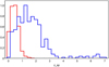 |
Fig. 1 Normalised histogram of spectroscopic redshift (z_sp) distribution for the used sample of galaxies (red line) and QSOs (blue line). |
3 Random forest classifier
In this work, we use a RF classifier (Breiman 2001), which consists in applying a set of independent decision trees to perform the classification. Decision trees are among the most commonly used machine-learning algorithms because they are simple to use and their results are easy to interpret in comparison with other black box models such as artificial neural networks. However, counterbalancing these advantages is a lack of robustness: small changes in the training data may lead to large changes in the final results. RFs, on the other hand, overcome this limitation because they use many decision trees, which are trained on random subsets of the training data, and the final classification is more robust because it is the result of the full set of learning processes and not only one tree.
We use the Scikit-Learn1 (Pedregosa et al. 2011) library to build our models. The two main parameters when using a RF classifier are the number of trees in the forest (n_estimators) and the size of the random subset of features to be used (max_features). In principle, the greater the value of n_estimators, the better the results, but there is a n_estimators value beyond which the results do not change significantly. The default value for n_estimators in the Scikit-Learn library is n_estimators = 100, which we keep as a ‘reference’ value (the effect of the free parameters on the results is discussed in Sect. 4.1). According to the Scikit-Learn tutorial, an empirical good value of max_features for classification tasks is the square root of the total number of available features. For the ALHAMBRA survey (with 23 filters), this approximately corresponds to max_features = 5, which will be our reference value for this parameter. Another important parameter is the maximum allowed depth of the trees (max_depth). By default, Scikit-Learn sets this value to none, that is, it allows the trees to be to fully developed. For the moment, we choose max_depth = 10 as the reference value and we leave a discussion of the free parameters to Sect. 4.1.
There are other less relevant parameters, such as the minimum number of samples required to split an internal node of the tree, the minimum impurity decrease necessary to split a node, or the function used to measure the quality of the split, either gini (the default criterion in Scikit-Learn) or entropy. We ran several tests in which we varied these parameters and, beyond computing performance, the final results are statistically similar, and so for the most partwe kept these free parameters unchanged from their default (Scikit-Learn) values.
Regarding data samples, we balanced the sizes of the different classes to prevent any bias in the results and we used a cross-validation splitting strategy (we kept the default fivefold cross validation given by Scikit-Learn) to train and evaluate the performance of the RF classifier. With these considerations, the classifier has a total of about 1240 objects to be trained. Although increasing the training sample should result in a better classification, the optimal training size (i.e. the minimum size leading to a ‘good’ classification) depends on several factors, including, for instance, the number of input features (Maxwell et al. 2018). However, in comparison with other classifiers, RF seems to show a negligible decrease in its overall accuracy when training samples are reduced to sizes as small as approximately 300 samples (Ramezan et al. 2021). A key aspect of our approach is to keep the properties of the training and testing samples unaltered in order to be able to evaluate the real effects – on the classification – of using magnitudes instead of colours, broad instead of narrow bands as features, or different classification algorithms.
4 Results and discussion
In this section, we discuss our main results regarding the effect of the free parameters and the effect of using different features and data sets on the classification performance. We perform a more detailed analysis of results obtained when using colours from the ALHAMBRA survey as features. In order to evaluate the global performance of the classifier, we use the accuracy (AC) as the main metric, which is a simple and direct measure giving the fraction of well-classified objects (stars, galaxies, and QSOs), that is, the number of true positives and true negatives divided by the total number of objects. We also calculate and show other metrics of interest for each object class, such as precision (i.e. the fraction of positive predictions that are actually positive), recall (the fraction of positive data that is predicted to be positive), and F1-score (the harmonic mean of precision and recall). We pay special attention to the QSO precision (QP), that is, the fraction of QSOs that are well classified, because we are particularly interested in generating a sample of QSO candidates that is as free of stars and galaxies as possible. For each classifier execution, we determine mean values and uncertainties associated to each metric, which is important for validating whether metric differences are statistically significant or not.
4.1 Free parameter effects
As mentioned above, our reference cases are the ones for which criterion = gini, n_estimators = 100, max_features = 5, and max_depth = 10. If the RF classifier is executed using these parameters and the 23 bands of the ALHAMBRA photometric catalogue, we obtain that AC = 0.779 ± 0.0072 and QP = 0.743 ± 0.009. These values are smaller than those found by other authors. For example, Clarke et al. (2020) obtained QP ≃ 0.89–0.96 depending on the used features (SDSS or WISE magnitudes, or a combination of both) for a sample of approximately 1.5 million spectroscopically confirmed sources. Differences in performance metrics come, among other things, from the difference in sample sizes. Final performances would indeed improve if additional features were incorporated, such as the photometric redshift estimations available in the ALHAMBRA Gold Catalogue (Molino et al. 2014), but in any case the exact range of obtained metrics is not of utmost importance because we are interested in evaluating the relative contributions of using magnitudes and colours of different band widths.
Figure 2 shows the effects of free-parameter variations on the obtained global accuracy. We see that, even though associated uncertainties decrease, AC remains almost unchanged as the number of trees in the forest increases. The same occurs with the maximum number of features used by the RF, where no significant differences are observed between using almost the full set or only two features (photometric bands). This is not a surprising result, because the RF classifier found one relevant feature, the K band magnitude, with an importance index of 0.14, whereas the other features had smaller importance indices in the range 0.02–0.06. For the case of maximum tree depth, above a reasonable threshold value (max_features ≃ 8) we find that, again, the accuracy remains roughly the same.
We then wanted to investigate the possible outcome of using the standard strategy to search for the optimal combination of free parameters that yields the best classification. To this end, we applied the Scikit-Learn tool GridSearchCV, which considers a grid with all possible parameter combinations. We spanned the ranges n_estimators = 100–500, max_depth = 2– 20, max_f eatures = 2–20 and criterion = gini, entropy, and the optimal set of parameters obtained was n_estimators = 100, max_depth = 10, max_features = 18, and criterion = entropy. With these values, the RF yields an accuracy that is statistically identical to the reference case (AC = 0.779 ± 0.005). Furthermore, when using other features (colours) or datasets (SDSS), we find no significant differences between reference and optimal cases (Table 1 in the following section).
4.2 Different features and datasets
Our main results regarding the global performance of the RF classifier are summarised in Table 1, where we can compare the results obtained for different features (either magnitudes or colours), sets of filters (ALHAMBRA or SDSS3), and sets of free parameters (reference or optimal). The corresponding metrics for each class are shown in Table 2.
There are no significant differences between using the optimal set of parameters estimated by GridSearchCV and any other reasonable combination of free parameters, including our reference combination, which is shown in Table 1. Also, if magnitudes from a system with narrower filters, such as ALHAMBRA, are used, the results are marginally better (AC ~ 0.78) than using magnitudes from SDSS (AC ~ 0.77). It seems clear that using colours instead of magnitudes results in better performances of the classifier. The best performance (AC ~ 0.88–0.90) occurs when colours from a narrow-band system such as ALHAMBRA are used as features. In this case, the global accuracy is >10 standard deviations higher than using magnitudes as features.
The latter result is expected, in principle, because from a photometric point of view the difference between QSOs and other objects like galaxies and stars should be reflected in their spectral energy distributions (SEDs), and the shape of the SEDs can be described through colours. The classification algorithm works by comparing features, and it could be considered that comparing magnitudes is equivalent, in some way, to working with colours. However, our results indicate that a better classification is obtained when colours are used directly as input for the RF classifier. Additionally, colours calculated using narrow bandwidths more accurately describe the SED shape, and that is likely the reason why we get better performances with ALHAMBRA than with SDSS.
Regarding the performance for each class (Table 2), we can see that all the metrics yield significantly higher values and lower associated uncertainties when colours from ALHAMBRA are used as features, which seems to indicate that using narrow band colours as inputs tends to produce more robust results. Moreover, in concordance with the results in Table 1, there is no or little difference between using the optimal or the reference set of free parameters. For the best results, that is, those corresponding to colours from ALHAMBRA, the values of precision, recall, and F1-score for the different classes (QSO, GAL, STA) are always in the range ~0.85–0.95. QSO and GAL results are quite similar, whereas STA metrics tend to give better values. In fact, stars always yield better metrics for any combination of features or databases and this is a reasonable result because, in general, star colours in our working sample tend to be different from those of galaxies and QSOs (see e.g. Fig. 5).
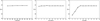 |
Fig. 2 Global accuracy (AC) as a function of free parameters n_estimators (left panel), max_features (central panel), and max_depth (right panel) when the RF classifier is applied with magnitudes from ALHAMBRA as features. In each case, the rest of the free parameters are fixed to their reference values (see text). Error bars correspond to three times the estimated standard deviations. |
Accuracy (AC) and its standard deviation (in brackets) obtained for different combinations of features, databases, and freeparameter sets.
4.3 Results using colours from the ALHAMBRA catalogue
Our most accurate results were obtained when colours from the ALHAMBRA catalogue were used as features in the RF classifier. Given that there is a total of 23 filters, the number of available colours is 253. Mean global accuracy and QSO precision for the reference case were AC = 0.878 ± 0.004 and QP = 0.860 ± 0.007, respectively (Tables 1 and 2). Figure 3 shows the confusion matrix for the first random execution using the reference parameter configuration. We see that, even for our relatively small training sample size, the model provides a good classification. The precision obtained in this execution for QSOs, galaxies, and stars was 0.88, 0.84, and 0.91, respectively. As mentioned above, stars were always better classified than QSOs and galaxies. The corresponding feature importances are shown in Fig. 4. Colours that contribute the most to the overall classification are the reddest ones and those using the K-band, in particular J–K, F923W–K, H–K, F706W–F768W, and F706W–F799W are the five most relevant features. Figure 5 shows as an example the F706W – F799W versus J–K plot for our working sample. We can see that J–K is a useful feature for separating stars because, in general, galaxies and QSOs tend to be redder than stars. This result agrees with Bai et al. (2019), who found that IR colours, such as those involving JHK bands, play an important role in star–galaxy–QSO classification with RFs. Similarly, Nakoneczny et al. (2021) noted the importance of NIR JHK-bands using XGBoost models based on colours and magnitude ratios. Our results also point out the convenience of using IR colours – which are less affected by dust than optical ones – for classifying QSOs when using only photometric information, and the same conclusion was obtained when we used SDSS and JHK bands exclusively. Misclassified sources (marked as open symbols in Fig. 5) tend to be spread over the colour–colour regions where different classes coexist without any obvious bias. Mis-classified QSOs (open circles in the example shown in Fig. 5) represent ≃18% of the total QSO sample. From this, those classified as galaxies (~11%) are QSOs, which in the colour–colour diagram tend to be located near the region where most of galaxies are found. A similar behaviour occurs for QSOs that are incorrectly classified as stars (~7%). We are particularly interested in identifying the galaxies and stars that are misclassified as QSOs, because these are the sources that may contribute to contaminating any potential catalogue of QSO candidates. All misclassified stars (≃3.5% of the star sample, which are plotted as open squares in the example shown in Fig. 5) are of spectral type F or later, but these stars are incorrectly identified as galaxies and not as QSOs. Instead, ≃12% of the galaxies are incorrectly labelled as QSOs, whether they are normal galaxies (≃7%) or starburst galaxies (≃5%) according to SDSS.
Precision, recall, and F1 metrics with their standard deviations (in brackets) obtained for different combinations of features, databases, and free parameter sets, and for each of the classes in the sample: quasars (QSO), galaxies (GAL), and stars (STA).
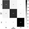 |
Fig. 3 Resulting confusion matrix of predicted and true classes for the first random execution of the RF using ALHAMBRA colours as features and the standard set of free parameters. |
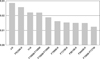 |
Fig. 4 Relative importance of the features (colours) for the same execution shown in Fig. 3. For clarity, only the ten most important features are presented. |
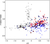 |
Fig. 5 Colour–colour diagram, F706W – F799W versus J–K, for all stars (grey solid squares), galaxies (red solid triangles), and QSOs (blue solid circles) in the sample, for the same execution shown in Fig. 3. Mis-classified sources are also plotted as open symbols for stars (squares), galaxies (triangles), and QSOs (circles). |
4.4 Results using colours from the SDSS catalogue
When photometry from SDSS combined with the JHK bands is used by the classifier, metric values tend to be smaller than those for ALHAMBRA photometry. As before, using colours instead of magnitudes yields better performances, although these are still not as good as those achieved when using colours from ALHAMBRA (see Tables 1 and 2). Global accuracy when using SDSS colours is around AC ≃ 0.79 and the QSO precision gives QP ≃ 0.75–0.76. Stars are once again the best classified class with precision values of around 0.9. As in the previous section, misclassified stars are exclusively classified as galaxies, not as QSOs, whereas ≲15% of the galaxies present in the sample are incorrectly identified as QSOs. These results are very similar to the ones obtained with ALHAMBRA colours. The reason for this is that the main colours contributing to the classification include the JHK bands that are common to both of our databases. The importance of the SDSS colours used as predictors by the classifier is shown in Fig. 6, where we can see that H–K and J–K clearly stand out as the two most important features, which are also identified as important features from the ALHAMBRA database. The significantly better performance with colours from ALHAMBRA (in comparison with SDSS) is likely related to the additional narrow-band colours that more accurately describe the shapes of the different SEDs.
5 Comparison with different algorithms
The results presented above suggest that, apart from having a high-quality training set, a key ingredient for a relatively good photometric classification of QSOs is the use of colours instead of magnitudes as input data. The set of filters used does not necessarily have to be very large, but it should include IR bands. Instead, the classification model itself and the exact values of its free parameters do not seem to play an important role. In order to verify this, we ran several experiments using other common supervised classifiers. Although the analysis in this section is not as detailed as for RF, we tested different configurations, free parameter sets, and parameter optimisation strategies. For a consistent comparison with our previous results for RF, we kept the characteristics of the training and testing sets unaltered. As input features, we used either the full set of available colours from ALHAMBRA or SDSS, or the corresponding ten most relevant ones shown in Figs. 4 or 6. The classification algorithms that we studied are:
K-nearest neighbours (KNN);
gradient boosting (GBoost);
support vector classifier (SVC);
feedforward neural networks (FNN).
All the models (except FNN) were implemented with the same previously used Scikit-Learn library (Pedregosa et al. 2011) and, in each case, we used k-fold cross-validation with shuffling and calculated the global accuracy and the other relevant metrics (precision, recall and F1-score) for each of the classes. For the case of neural networks, we used a single-layer FNN implemented with the nnet package on R (Ripley 1996; Venables & Ripley 2002) with its default options (logistic output units, least squares fitting) as the method for supervised training. The inputs to the neural network were the ten most relevant colours (Figs. 4 or 6) and the network was configured with ten input neurons, five neurons in the hidden layer, and one output neuron. From the full set of executions with different parameters and criteria specific to each model, we keep and show the best result of each classifier, which is summarised in Table 3.
We obtained that classifier performances were close to each other and global accuracies are compatible within associated uncertainties. Stars tend to be better classified (i.e. with greater precision) than galaxies and QSOs by all the algorithms except FNN. This is likely due to the fact that, in general, intrinsic shapes of star SEDs and therefore their colours differ more than those of galaxies and QSOs (see e.g. Fig. 5). Global performances for each algorithm are better for ALHAMBRA colours than for SDSS colours. Best overall performance for ALHAMBRA colours is achieved by GBoost with AC = 0.86, which is not too far from the obtained RF accuracy (AC = 0.88–0.90); this not a surprising result considering that RF and GBoost, despite being trained in different ways, are both based on multiple decision trees. From the point of view of QSO classification, RF with ALHAMBRA colours and the optimal parameter set seems to show a better performance (QP ≃ 0.89) than the other methods; although, strictly speaking, the difference between RF and KNN, GBoost, and SVC is ≲3 standard deviations. The exception to these results and behaviours is FNN with a higher accuracy for SDSS colours than for ALHAMBRA colours and a relatively small precision value when using ALHAMBRA colours (QP ≃ 0.69), which is likely associated to the sensitivity of neural networks to small training datasets. FNN results could be improved by optimising the network through its topology. This could be achieved, for example, with another layer of hidden neurons, but this is beyond the goals of the present work.
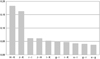 |
Fig. 6 Relative importance of the SDSS colours for the reference case. Only the ten most relevant colours are shown. |
Global accuracy (AC), precision, recall, and F1 metrics with their standard deviations σ (in brackets) obtained with different algorithms using either ALHAMBRA or SDSS colours.
6 Conclusions
In this work, we systematically evaluated the performance of RFs in classifying QSOs, galaxies, and stars using either magnitudes or colours – both from broad and narrow-band filters – as features. Our main results are summarised in Tables 1 and 2. The effect of varying free parameters (within reasonable ranges of values), such as the number of random trees, their maximum depths, or the maximum number of used features, is negligible, and the results (global accuracy and class precision) are always the same within their associated uncertainties. Using colours instead of magnitudes as features results in better performances of the classifier, especially using colours from ALHAMBRA. However, colours that contribute the most to the classification are those that contain the JHK bands, which is in agreement with results found by other authors. The best performance (that using colours from ALHAMBRA) yields an accuracy of around 0.88–0.90 and a QSO precision of 0.86–0.89, depending on the free parameters used. From this work, we can conclude that in order to accurately identify QSOs from photometric data exclusively, it is important to use a set of colours that includes IR bands and a good input dataset, whereas the classification model and the exact value of its free parameters are of less importance in obtaining accurate results. Upcoming large-scale surveys, such as J-PAS (Benitez et al. 2014), which will observe through 54 narrow-band filters, would seem to be appropriate as input data for machine-learning algorithms that use photometric colours to search for new QSOs. However, the results of this work suggest that a much smaller subset of colours that includes NIR bands would be sufficient.
Acknowledgements
We are very grateful to the referee for his/her careful reading of the manuscript and helpful comments and suggestions, which improved this paper. NS acknowledges financial support from the Spanish Ministerio de Cien-cia, Innovación y Universidades through grant PGC2018-095049-B-C21. During this work we have made extensive use of TOPCAT (Taylor 2005).
References
- Abdurro’uf, Accetta, K., Aerts, C., et al. 2022, ApJS, 259, 35 [NASA ADS] [CrossRef] [Google Scholar]
- Bai, Y., Liu, J., Wang, S., & Yang, F. 2019, AJ, 157, 9 [Google Scholar]
- Ball, N. M., Brunner, R. J., Myers, A. D., & Tcheng, D. 2006, ApJ, 650, 497 [NASA ADS] [CrossRef] [Google Scholar]
- Benitez, N., Dupke, R., Moles, M., et al. 2014, arXiv e-prints [arXiv:1403.5237] [Google Scholar]
- Breiman, L. 2001, Mach. Learn., 45, 5 [Google Scholar]
- Carrasco, D., Barrientos, L. F., Pichara, K., et al. 2015, A&A, 584, A44 [NASA ADS] [CrossRef] [EDP Sciences] [Google Scholar]
- Clarke, A. O., Scaife, A. M. M., Greenhalgh, R., & Griguta, V. 2020, A&A, 639, A84 [NASA ADS] [CrossRef] [EDP Sciences] [Google Scholar]
- Cunha, P. A. C., & Humphrey, A. 2022, A&A, 666, A87 [NASA ADS] [CrossRef] [EDP Sciences] [Google Scholar]
- Flesch, E. W. 2021, ApJ, submitted [arXiv:2105.12985] [Google Scholar]
- Glikman, E., Lacy, M., LaMassa, S., et al. 2022, ApJ, 934, 119 [NASA ADS] [CrossRef] [Google Scholar]
- Guarneri, F., Calderone, G., Cristiani, S., et al. 2021, MNRAS, 506, 2471 [NASA ADS] [CrossRef] [Google Scholar]
- Khramtsov, V., Spiniello, C., Agnello, A., & Sergeyev, A. 2021, A&A, 651, A69 [NASA ADS] [CrossRef] [EDP Sciences] [Google Scholar]
- Kovàcs, A., & Szapudi, I. 2015, MNRAS, 448, 1305 [CrossRef] [Google Scholar]
- Krakowski, T., Malek, K., Bilicki, M., et al. 2016, A&A, 596, A39 [NASA ADS] [CrossRef] [EDP Sciences] [Google Scholar]
- Li, C., Zhang, Y., Cui, C., et al. 2021, MNRAS, 506, 1651 [NASA ADS] [CrossRef] [Google Scholar]
- Makhija, S., Saha, S., Basak, S., & Das, M. 2019, Astron. Comput., 29, 100313 [NASA ADS] [CrossRef] [Google Scholar]
- Maxwell, A. E., Warner, T. A., & Fang, F. 2018, Int. J. Rem. Sens., 39, 2784 [NASA ADS] [CrossRef] [Google Scholar]
- Moles, M., Benítez, N., Aguerri, J. A. L., et al. 2008, AJ, 136, 1325 [NASA ADS] [CrossRef] [Google Scholar]
- Molino, A., Benítez, N., Moles, M., et al. 2014, MNRAS, 441, 2891 [Google Scholar]
- Nakazono, L., Mendes de Oliveira, C., Hirata, N. S. T., et al. 2021, MNRAS, 507, 5847 [CrossRef] [Google Scholar]
- Nakoneczny, S., Bilicki, M., Solarz, A., et al. 2019, A&A, 624, A13 [NASA ADS] [CrossRef] [EDP Sciences] [Google Scholar]
- Nakoneczny, S. J., Bilicki, M., Pollo, A., et al. 2021, A&A, 649, A81 [NASA ADS] [CrossRef] [EDP Sciences] [Google Scholar]
- Pedregosa, F., Varoquaux, G., Gramfort, A., et al. 2011, J. Mach. Learn. Res., 12, 2825 [Google Scholar]
- Peng, N., Zhang, Y., Zhao, Y., & Wu, X.-B. 2012, MNRAS, 425, 2599 [NASA ADS] [CrossRef] [Google Scholar]
- Ramezan, C. A., Warner, T. A., Maxwell, A. E., & Price, B. S. 2021, Rem. Sens., 13, 368 [NASA ADS] [CrossRef] [Google Scholar]
- Ripley, B. D. 1996, Pattern Recognition and Neural Networks (Cambridge University Press) [CrossRef] [Google Scholar]
- Schindler, J.-T., Fan, X., Huang, Y.-H., et al. 2019, ApJS, 243, 5 [NASA ADS] [CrossRef] [Google Scholar]
- Skrutskie, M. F., Cutri, R. M., Stiening, R., et al. 2006, AJ, 131, 1163 [NASA ADS] [CrossRef] [Google Scholar]
- Suchkov, A. A., Hanisch, R. J., & Margon, B. 2005, AJ, 130, 2439 [NASA ADS] [CrossRef] [Google Scholar]
- Taylor, M. B. 2005, in Astronomical Data Analysis Software and Systems XIV, eds. P. Shopbell, M. Britton, & R. Ebert, Astronomical Society of the Pacific Conference Series, 347, 29 [NASA ADS] [Google Scholar]
- Vasconcellos, E. C., de Carvalho, R. R., Gal, R. R., et al. 2011, AJ, 141, 189 [Google Scholar]
- Venables, W. N., & Ripley, B. D. 2002, Modern Applied Statistics with S (Springer) [Google Scholar]
- Wang, C., Bai, Y., López-Sanjuan, C., et al. 2022, A&A, 659, A144 [Google Scholar]
- Wenzl, L., Schindler, J.-T., Fan, X., et al. 2021, AJ, 162, 72 [NASA ADS] [CrossRef] [Google Scholar]
- Wright, E. L., Eisenhardt, P. R. M., Mainzer, A. K., et al. 2010, AJ, 140, 1868 [Google Scholar]
- Yèche, C., Petitjean, P., Rich, J., et al. 2010, A&A, 523, A14 [NASA ADS] [CrossRef] [EDP Sciences] [Google Scholar]
- York, D. G., Adelman, J., Anderson, J., John E., et al. 2000, AJ, 120, 1579 [NASA ADS] [CrossRef] [Google Scholar]
We are expressing associated uncertainties as one standard deviation.
For a proper comparison, in this work, SDSS photometry is always used in combination with the JHK bands that are also included in the ALHAMBRA catalogue.
All Tables
Accuracy (AC) and its standard deviation (in brackets) obtained for different combinations of features, databases, and freeparameter sets.
Precision, recall, and F1 metrics with their standard deviations (in brackets) obtained for different combinations of features, databases, and free parameter sets, and for each of the classes in the sample: quasars (QSO), galaxies (GAL), and stars (STA).
Global accuracy (AC), precision, recall, and F1 metrics with their standard deviations σ (in brackets) obtained with different algorithms using either ALHAMBRA or SDSS colours.
All Figures
|
Fig. 1 Normalised histogram of spectroscopic redshift (z_sp) distribution for the used sample of galaxies (red line) and QSOs (blue line). |
| In the text | |
|
Fig. 2 Global accuracy (AC) as a function of free parameters n_estimators (left panel), max_features (central panel), and max_depth (right panel) when the RF classifier is applied with magnitudes from ALHAMBRA as features. In each case, the rest of the free parameters are fixed to their reference values (see text). Error bars correspond to three times the estimated standard deviations. |
| In the text | |
|
Fig. 3 Resulting confusion matrix of predicted and true classes for the first random execution of the RF using ALHAMBRA colours as features and the standard set of free parameters. |
| In the text | |
|
Fig. 4 Relative importance of the features (colours) for the same execution shown in Fig. 3. For clarity, only the ten most important features are presented. |
| In the text | |
|
Fig. 5 Colour–colour diagram, F706W – F799W versus J–K, for all stars (grey solid squares), galaxies (red solid triangles), and QSOs (blue solid circles) in the sample, for the same execution shown in Fig. 3. Mis-classified sources are also plotted as open symbols for stars (squares), galaxies (triangles), and QSOs (circles). |
| In the text | |
|
Fig. 6 Relative importance of the SDSS colours for the reference case. Only the ten most relevant colours are shown. |
| In the text | |
Current usage metrics show cumulative count of Article Views (full-text article views including HTML views, PDF and ePub downloads, according to the available data) and Abstracts Views on Vision4Press platform.
Data correspond to usage on the plateform after 2015. The current usage metrics is available 48-96 hours after online publication and is updated daily on week days.
Initial download of the metrics may take a while.