| Issue |
A&A
Volume 687, July 2024
|
|
|---|---|---|
| Article Number | A223 | |
| Number of page(s) | 10 | |
| Section | Interstellar and circumstellar matter | |
| DOI | https://doi.org/10.1051/0004-6361/202450087 | |
| Published online | 16 July 2024 | |
Planet-driven spirals in protoplanetary discs: Limitations of the semi-analytical theory for observations
1
Univ. Grenoble Alpes, CNRS, IPAG,
38000
Grenoble,
France
2
Université Côte d’Azur, Observatoire de la Côte d’Azur, CNRS, Laboratoire Lagrange,
France
e-mail: daniele.fasano@oca.eu
3
Dipartimento di Fisica, Università degli Studi di Milano,
Via Celoria 16,
Milano,
Italy
4
School of Physics and Astronomy, Monash University,
Clayton,
Vic 3800,
Australia
5
European Southern Observatory (ESO),
Karl-Schwarzschild-Strasse 2,
85748
Garching bei Munchen,
Germany
6
INAF, Osservatorio Astrofisico di Arcetri,
50125
Firenze,
Italy
7
Leiden Observatory, Leiden University,
PO Box 9513,
2300
RA
Leiden,
The Netherlands
8
Department of Astronomy, University of Florida,
Gainesville,
FL
32611,
USA
Received:
22
March
2024
Accepted:
27
May
2024
Context. Detecting protoplanets during their formation stage is an important but elusive goal of modern astronomy. Kinematic detections via the spiral wakes in the gaseous disc are a promising avenue to achieve this goal.
Aims. We aim to test the applicability of a commonly used semi-analytical model for planet-induced spiral waves to observations in the low and intermediate planet mass regimes. In contrast to previous works that proposed using the semi-analytical model to interpret observations, in this study we analyse for the first time both the structure of the velocity and density perturbations. Methods. We ran a set of FARGO3D hydrodynamic simulations and compared them with the output of the semi-analytic model in the code WAKEFLOW. We divided the disc into two regions. We used the density and velocity fields from the simulation in the linear region, where density waves are excited. In the non-linear region, where density waves propagate through the disc, we then solved Burgers’ equation to obtain the density field, from which we computed the velocity field.
Results. We find that the velocity field derived from the analytic theory is discontinuous at the interface between the linear and nonlinear regions. After ~0.2 rp from the planet, the behaviour of the velocity field closely follows that of the density perturbations. In the low mass limit, the analytical model is in qualitative agreement with the simulations, although it underestimates the azimuthal width and the amplitude of the perturbations, predicting a stronger decay but a slower azimuthal advance of the shock fronts. In the intermediate regime, the discrepancy increases, resulting in a different pitch angle between the spirals of the simulations and the analytic model.
Conclusions. The implementation of a fitting procedure based on the minimisation of intensity residuals is bound to fail due to the deviation in pitch angle between the analytic model and the simulations. In order to apply this model to observations, it needs to be revisited so that it can also account for higher planet masses.
Key words: methods: analytical / planets and satellites: formation / protoplanetary disks / planet–disk interactions
© The Authors 2024
 Open Access article, published by EDP Sciences, under the terms of the Creative Commons Attribution License (https://creativecommons.org/licenses/by/4.0), which permits unrestricted use, distribution, and reproduction in any medium, provided the original work is properly cited.
This article is published in open access under the Subscribe to Open model. Subscribe to A&A to support open access publication.
1 Introduction
The Atacama Large (sub-)Millimeter Array (ALMA) has proven to be fundamental in the study of stars and planet formation. Images of the millimetre dust emission have shown the presence of many substructures (rings, gaps, cavities, and spirals) in the vast majority of targeted discs (Andrews et al. 2018). Although these features can be associated with the presence of unseen planets, planet–disc interaction is not the only explanation behind the formation of these substructures. For instance, rings and gaps can be due to magneto-rotational instabilities (Flock et al. 2015) or dust sintering outside the snow line (Okuzumi et al. 2012). It is then difficult to unambiguously associate dust substructures with the presence of planets in a disc and study their properties. However, ALMA opened yet another window to study protoplanetary discs by means of kinematic signatures. As the planet interacts with the gas, it excites spiral density waves and perturbs the disc velocity field, leaving characteristic signatures in the molecular line emission (Disk Dynamics Collaboration 2020; Bollati et al. 2021; Pinte et al. 2023).
Kinematic studies searching for planet–disc interaction signatures in molecular line emission have been carried out in recent years and have followed different strategies. The effects of an embedded planet on the background velocity field may consist of deviations from Keplerian velocity in rotation curves of the gas (Teague et al. 2018), a Doppler flip in the first moment map (Pérez et al. 2018), and deviations from the isovelocity curves (so-called kinks) in the channel maps (Perez et al. 2015). A technique based on the detection of this last deviation was successfully used to infer the presence of protoplanets in the systems HD 163296 (Pinte et al. 2018) and HD 97048 (Pinte et al. 2019) using the line emission of CO isotopologues. Currently, there are more than ten planet candidates waiting for confirmation that have been identified with this method (Pinte et al. 2023).
At the moment, however, the only way to obtain an estimate of the planet mass with this technique is through a comparison between observations and computationally expensive and time-consuming numerical simulations (Pinte et al. 2019). In the case of HD 163296 and HD 97048, planet mass estimates lie between 2 and 3 MJ. As this procedure relies on numerical hydrodynamical simulations, it is not possible to quantify the error on this measurement in a statistical manner due to the high computational cost. To develop a statistically significant procedure for the evaluation of the planet mass using Markov chain Monte Carlo methods, an analytical model for planet-produced kinks is needed.
Planetary kinks are a result of the density wave perturbations generated by a planet. The first linear theory describing the propagation of density waves in a gaseous disc excited by a planet was developed by Goldreich & Tremaine (1979, 1980), and Papaloizou & Lin (1984). The perturbing planet excites density waves at Lindblad resonant locations, which undergo constructive interference and form the planetary spiral wake (Ogilvie & Lubow 2002). Goodman & Rafikov (2001) and Rafikov (2002) first complemented the linear theory by using a shearing box for the excitation of planetary spiral wakes and a non-linear, semi-analytic framework describing its propagation. Miranda & Rafikov (2019, 2020) then generalised the linear theory, moving from the shearing sheet approximation to a global model. Finally, the non-linear model was expanded in order to also account for the velocity perturbations in Bollati et al. (2021).
The linear excitation of the wake close to the planet and its non-linear propagation in the rest of the disc can naturally be separated into two regimes when the planet mass satisfies Mp ≲ mth, where the thermal mass mth is
![$\[m_{\mathrm{th}}=\frac{2}{3} \frac{c_{\mathrm{s}}^3}{\Omega G}=\frac{2}{3}\left(\frac{h_{\mathrm{p}}}{r_{\mathrm{p}}}\right)^3 M_{\star}.\]$](/articles/aa/full_html/2024/07/aa50087-24/aa50087-24-eq1.png) (1)
(1)
Here, cs is the sound speed, Ω is the orbital frequency, hp is the disc scale height, rp is the planet radial position, and M* is the stellar mass. The thermal mass for realistic parameters (hp/rp ~ 0.1, M* ~ 1 M⊙) is generally on the order of a Jupiter mass, which is in the range of the planet mass estimates obtained from the observations (Pinte et al. 2018, 2019). The accuracy of the model in the low planet mass limit has been tested in Cimerman & Rafikov (2021), focusing only on the density structure of the spiral.
However, observed planet candidates from continuum substructures (Bae et al. 2023; Lodato et al. 2019) and molecular line emission (Pinte et al. 2023) need to be massive enough to create strong detectable signatures, often exceeding the thermal mass. With this paper, we aim to assess the applicability of the model to observations when approaching the thermal mass (Mp ~ 1 mth), a region of interest for ongoing observational surveys such as the ALMA large program exoALMA. In contrast to previous works, which proposed the use of the semi-analytical model to interpret observations, we focus on the velocity field in our analysis, as this is the quantity observed directly in the kinematic campaigns. In order to do so, we performed 2D numerical hydrodynamical simulations of a gaseous protoplanetary disc, considering different values of the planet mass, that we then compared with the results obtained with the semi-analytical model. We quantitatively analysed the profiles of the azimuthal perturbations, focusing on the pitch angle of the spirals.
This paper is organised as follows: in Sect. 2, we briefly summarise the semi-analytical model, and we describe the numerical setup we used to test its accuracy. Section 3 presents the comparison between the model and the hydrodynamical simulations. Finally, we draw our conclusions in Sect. 4.
2 Methods
In this section, we summarise the key points of the semi-analytic model and the main improvements with respect to previous iterations. Then we introduce the numerical setup of the hydrodynamic simulations.
2.1 Semi-analytical model
2.1.1 Background disc
We considered an unperturbed 2D disc in a cylindrical coordinate system (r, Φ) rotating around a star with mass M*. The hydrodynamical variables needed to solve the following equations:
![$\[\frac{\partial \Sigma_0}{\partial t}+\nabla \cdot\left(\Sigma_0 \mathbf{v}\right)=0,\]$](/articles/aa/full_html/2024/07/aa50087-24/aa50087-24-eq2.png) (2)
(2)
![$\[\frac{\partial \mathbf{v}}{\partial t}+(\mathbf{v} \cdot \nabla) \mathbf{v}=-\frac{1}{\Sigma_0} \nabla P-\nabla \Phi,\]$](/articles/aa/full_html/2024/07/aa50087-24/aa50087-24-eq3.png) (3)
(3)
where Σ0 is the surface density, v = (vr, vφ) is the velocity field, P is the pressure of the gas, and Φ ≡ –GM*/r is the gravitational potential of the star. We assumed radial power laws for the sound speed c0 and the surface density
![$\[c_0=c_{\mathrm{p}}\left(\frac{r}{r_{\mathrm{p}}}\right)^{-q},\]$](/articles/aa/full_html/2024/07/aa50087-24/aa50087-24-eq4.png) (4)
(4)
![$\[\Sigma_0=\Sigma_{\mathrm{p}}\left(\frac{r}{r_{\mathrm{p}}}\right)^{-p},\]$](/articles/aa/full_html/2024/07/aa50087-24/aa50087-24-eq5.png) (5)
(5)
where cp ≡ c0(rp) and Σp ≡ Σ0(rp). We considered a polytropic equation of state:
![$\[P=P_0\left(\frac{\Sigma}{\Sigma_0}\right)^\gamma,\]$](/articles/aa/full_html/2024/07/aa50087-24/aa50087-24-eq6.png) (6)
(6)
with γ as the adiabatic index, which implies a perturbed sound speed,
![$\[c^2=\frac{\partial P}{\partial \Sigma}=c_0^2(r)\left(\frac{\Sigma}{\Sigma_0}\right)^{\gamma-1}.\]$](/articles/aa/full_html/2024/07/aa50087-24/aa50087-24-eq7.png) (7)
(7)
The model we introduce in Sect. 2.1.2 was built assuming Eqs. (6)–(7). We then took the limit for γ → 1 to obtain locally isothermal discs and fixed q = 0 to recover globally isothermal discs.
We defined the disc aspect ratio
![$\[\frac{h}{r} \equiv \frac{c_0}{v_{\mathrm{K}}}=\frac{h_{\mathrm{p}}}{r_{\mathrm{p}}}\left(\frac{r}{r_{\mathrm{p}}}\right)^{1 / 2-q},\]$](/articles/aa/full_html/2024/07/aa50087-24/aa50087-24-eq8.png) (8)
(8)
where we used Eq. (4) in the second equality; vK = (GM*/r)1/2 is the Keplerian velocity, and we defined hp/rp ≡ cp(GM*/rp)−1/2.
Then, for a Keplerian power law disc, the gas rotates around the star with sub-Keplerian velocity, with radial and azimuthal components (Armitage 2015):
![$\[v_{r, 0}=0,\]$](/articles/aa/full_html/2024/07/aa50087-24/aa50087-24-eq9.png) (9)
(9)
![$\[v_{\varphi, 0}=v_{\mathrm{K}}\left[1-a\left(\frac{h_{\mathrm{p}}}{r_{\mathrm{p}}}\right)^2\left(\frac{r}{r_{\mathrm{p}}}\right)^b\right]^{1 / 2},\]$](/articles/aa/full_html/2024/07/aa50087-24/aa50087-24-eq10.png) (10)
(10)
where we have defined the coefficient a ≡ p + q + 3/2, the exponent b ≡ 1 − 2q, and the disc aspect ratio at the planet location hp/rp = h/r(rp).
2.1.2 Planet-induced perturbations
We modelled the density and velocity perturbations induced by a planet embedded in a 2D gas disc starting from the semi-analytical method outlined in Bollati et al. (2021), which is based on the framework first introduced in Goodman & Rafikov (2001) and Rafikov (2002). We expanded on this model by removing some of the original approximations from Bollati et al. (2021). In the following, we summarise the main points of this method, the limitations of the original approach of Bollati et al. (2021), and how we improve on it.
The shape of the wake generated by the planet in the linear approximation resulting from constructive interference of density waves excited at Lindblad resonant locations (Rafikov 2002; Ogilvie & Lubow 2002) is given by
![$\[\varphi_{\text {wake }}^{\text {linear }}=\varphi_{\mathrm{p}}+\operatorname{sgn}\left(r-r_{\mathrm{p}}\right) \int_{r_{\mathrm{p}}}^r \frac{\Omega\left(r^{\prime}\right)-\Omega_{\mathrm{p}}}{c_0\left(r^{\prime}\right)} \mathrm{d} r^{\prime} \text {, }\]$](/articles/aa/full_html/2024/07/aa50087-24/aa50087-24-eq11.png) (11)
(11)
where (rp, φp) are the planet coordinates in a polar reference frame centred on the star location; Ω(r) and Ωp ≡ Ω(rp) are the disc and planet angular velocities, respectively; and c0(r) is the sound speed of the unperturbed disc. Assuming Keplerian rotation and a constant disc aspect ratio, by substituting the power law prescription (Eq. (4)), Eq. (11) becomes (Rafikov 2002)
![$\[\begin{aligned}\varphi_{\text {wake }}^{\text {linear }}= & \varphi_{\mathrm{p}}+\operatorname{sgn}\left(r-r_{\mathrm{p}}\right)\left(\frac{h_{\mathrm{p}}}{r_{\mathrm{p}}}\right)^{-1}\left[\frac{\left(r / r_{\mathrm{p}}\right)^{q-1 / 2}}{q-1 / 2}+\right. \\& \left.-\frac{\left(r / r_{\mathrm{p}}\right)^{q+1}}{q+1}-\frac{3}{(2 q-1)(q+1)}\right].\end{aligned}\]$](/articles/aa/full_html/2024/07/aa50087-24/aa50087-24-eq12.png) (12)
(12)
This linear prescription does not take into account the nonlinear effects arising after the perturbations’ shock. Cimerman & Rafikov (2021) introduced a non-linear correction to the spiral wake in the form
![$\[\varphi_{\text {wake }}^{\text {nonlinear }}=\varphi_{\text {wake }}^{\text {linear }}+\operatorname{sgn}\left(r-r_{\mathrm{p}}\right) \Delta \phi_0 \frac{h_{\mathrm{p}}}{r_{\mathrm{p}}} \sqrt{t-t_0} \text {, }\]$](/articles/aa/full_html/2024/07/aa50087-24/aa50087-24-eq13.png) (13)
(13)
where Δϕ0 ≃ 1. This value is obtained from a fit on their simulations in the range 0.05–0.5 mth.
The computation of the density perturbation was carried out in two distinct spatial regions: in an annulus centred on the planet position, where the density and velocity fields are obtained under the linear approximation, and further away from it, where the structure of the wake is calculated in the non-linear regime (Rafikov 2002). We defined the separation between these two regimes as follows:
![$\[r_{ \pm}=r_{\mathrm{p}} \pm 2 l_{\mathrm{p}}\]$](/articles/aa/full_html/2024/07/aa50087-24/aa50087-24-eq14.png) (14)
(14)
![$\[l_{\mathrm{p}}=\frac{2}{3} h_{\mathrm{p}}.\]$](/articles/aa/full_html/2024/07/aa50087-24/aa50087-24-eq15.png)
This value was chosen so that the linear region is large enough to include Lindblad resonances exciting the spiral waves, but it limits the non-linear effects that start appearing after the shock of the spiral waves(Goodman & Rafikov 2001)1.
2.1.3 Linear region
In the original model of Bollati et al. (2021), the density and velocity perturbations in the linear regime were obtained assuming the linear and shearing sheet approximations, following the procedure from Goodman & Rafikov (2001). However, by definition of the shearing sheet approximation, this linear solution is valid only in a square box centred on the planet position with sides on the order of lp. As a result, we find that the azimuthal extent of the box is not large enough to fully capture the density profile needed, which is an initial condition to solve Burgers’ equation in the non-linear regime.
An alternative approach has been presented in Miranda & Rafikov (2019, 2020). In their framework, the authors provide linear global density and velocity fields by solving a master equation for the enthalpy of the disc. In this way, it is then possible to extract the density profile along the entire azimuthal range and use it as the initial condition for the computation of the density field in the non-linear regime.
A third option consists of using both the density and velocity fields retrieved from numerical hydrodynamic simulations. Cimerman & Rafikov (2021) showed that the global linear solution is in good agreement with the simulation in the linear region and used the profile from the simulation as an initial condition to solve Burgers’ equation. In this paper, we follow the same approach and use the density and velocity fields from our hydro-dynamical simulations (see Sect. 2.2) in the annular region of width 4lp centred on the planet.
2.1.4 Non-linear region
In the non-linear regime, the equations are solved in a polar reference frame co-rotating with the planet. Rafikov (2002) showed that the structure of the density perturbation outside the linear region is described by the inviscid Burgers’ equation in a specific reference system with coordinates t, η
![$\[\partial_t \chi+\operatorname{sgn}\left(r-r_{\mathrm{p}}\right) \chi \partial_\eta \chi=0,\]$](/articles/aa/full_html/2024/07/aa50087-24/aa50087-24-eq16.png) (16)
(16)
![$\[t \equiv-\frac{r_{\mathrm{p}}}{l_{\mathrm{p}}} \frac{m_{\mathrm{p}}}{m_{\mathrm{th}}} \int_{r_{\mathrm{p}}}^r \frac{\Omega\left(r^{\prime}\right)-\Omega_{\mathrm{p}}}{c_0\left(r^{\prime}\right) g\left(r^{\prime}\right)} \mathrm{d} r^{\prime},\]$](/articles/aa/full_html/2024/07/aa50087-24/aa50087-24-eq17.png)
![$\[\eta \equiv \frac{r_{\mathrm{p}}}{l_{\mathrm{p}}}\left[\varphi-\varphi_{\text {wake }}(r)\right],\]$](/articles/aa/full_html/2024/07/aa50087-24/aa50087-24-eq18.png)
![$\[\chi \equiv \frac{\gamma+1}{2} \frac{\Sigma-\Sigma_0}{\Sigma_0} g(r),\]$](/articles/aa/full_html/2024/07/aa50087-24/aa50087-24-eq19.png)
![$\[g(r) \equiv \frac{2^{1 / 4}}{r_{\mathrm{p}} c_{\mathrm{p}} \Sigma_{\mathrm{p}}^{1 / 2}}\left(\frac{r \Sigma_0 c_0^3}{\left|\Omega-\Omega_{\mathrm{p}}\right|}\right)^{1 / 2},\]$](/articles/aa/full_html/2024/07/aa50087-24/aa50087-24-eq20.png)
with γ as the adiabatic index, χ representing the density perturbation, and the (t, η) coordinates representing the distance along the spiral wake and in the azimuthal direction with respect to the centre of the wake, respectively. In the case of a power-law Keplerian disc, using Eqs. (4)–(5), we can write Eqs. (17) and (20) as
![$\[t \equiv-\frac{3}{2^{5 / 4}\left(h_{\mathrm{p}} / r_{\mathrm{p}}\right)^{5 / 2}} \frac{m_{\mathrm{p}}}{m_{\mathrm{th}}} \int_1^{r / r_{\mathrm{p}}}\left(1-x^{3 / 2}\right)\left|1-x^{3 / 2}\right|^{1 / 2} x^w \mathrm{d} x,\]$](/articles/aa/full_html/2024/07/aa50087-24/aa50087-24-eq21.png) (21)
(21)
![$\[g(r) \equiv 2^{1 / 4}\left(\frac{h_{\mathrm{p}}}{r_{\mathrm{p}}}\right)^{1 / 2} \frac{\left(r / r_{\mathrm{p}}\right)^{5 / 4-(p+3 q) / 2}}{\left|1-\left(r / r_{\mathrm{p}}\right)^{3 / 2}\right|^{1 / 2}},\]$](/articles/aa/full_html/2024/07/aa50087-24/aa50087-24-eq22.png) (22)
(22)
where w = −11/4 + (p + 5q)/2.
The radial and azimuthal velocity perturbations can be related to the density perturbation χ with the following expressions:
![$\[v_r(r, \varphi)=\operatorname{sgn}\left(r-r_{\mathrm{p}}\right) \frac{2 c_0}{\gamma+1} \psi\]$](/articles/aa/full_html/2024/07/aa50087-24/aa50087-24-eq23.png) (23)
(23)
![$\[v_{\varphi}(r, \varphi)=\frac{c_0}{\left(\Omega-\Omega_{\mathrm{p}}\right) r} v_r,\]$](/articles/aa/full_html/2024/07/aa50087-24/aa50087-24-eq24.png) (24)
(24)
where we defined the mathematical quantity
![$\[\psi \equiv \frac{\gamma+1}{\gamma-1} \frac{c-c_0}{c_0}.\]$](/articles/aa/full_html/2024/07/aa50087-24/aa50087-24-eq25.png) (25)
(25)
By substituting Eq. (7), we can express ψ as a function of Σ
![$\[\psi=\frac{\gamma+1}{\gamma-1}\left[\left(\frac{\Sigma}{\Sigma_0}\right)^{(\gamma-1) / 2}-1\right].\]$](/articles/aa/full_html/2024/07/aa50087-24/aa50087-24-eq26.png) (26)
(26)
In the original model of Bollati et al. (2021), they assumed that the sound speed perturbation is a fraction of the unperturbed sound speed (ψ ≪ 1) and expanded Eq. (26) to the first order, obtaining approximate formulas for Eqs. (23)–(24). We found that the condition ψ ≪ 1 is not always satisfied, so we considered the exact transformation Eq. (26) to compute the velocity field in this paper.
We solved Eq. (16) following the method outlined in Bollati et al. (2021), using the density perturbation profile evaluated at the edge of the linear annulus as an initial condition. However, Bollati et al. (2021) solved Burgers’ equation only in the outer disc (i.e. for r > rp) and then copied the result in the inner disc (i.e. for r < rp). We improved on their approach by solving Burgers’ equation both in the outer and the inner disc, using as an initial condition, the density perturbation profile evaluated at the outer and inner edge of the linear annulus, respectively. The model was implemented in an open source code, WAKEFLOW2 (Hilder et al. 2023), which is used in the following analysis.
2.2 Numerical setup
We performed 2D hydrodynamical simulations using the code FARGO3D (Benítez-Llambay & Masset 2016; Masset 2000). We used the same setup described in Cimerman & Rafikov (2021) in order to compare our results in the low planet mass limit. Simulations were run in cylindrical coordinates on a meshed domain that extends radially between 0.2rp and 4rp with logarithmic spacing and uniformly over the full disc azimuthal extension. The grid resolution is Nϕ×Nr = 14400 × 6896, corresponding to a minimum of 50 cells per scale height at all simulated radii for each of our setups. We initialised each simulation in an axisymmetric state. To achieve centrifugal balance, we set the azimuthal component of the gas initial velocity to the Keplerian solution with the pressure support correction, while we set the radial component to zero. We initialised the surface density prescribing the radial profile as a power law of index −p. We used closed boundary conditions, implementing wave-killing zones near the radial boundaries for 0.2 ≤ r/rp ≤ 0.28 and 3.4 ≤ r/rp ≤ 4 to avoid reflections. In these regions, the gas density and radial velocity were relaxed towards their initial conditions, analogously to Val-Borro et al. (2006), on a timescale τ = 0.3/Ω(r).
We considered five simulations of a gas disc rotating around a 1 M⊙ star hosting a non-migrating and non-accreting planet with mass {0.25,1.0} mth to study the behaviour of the semi-analytic model in the low and intermediate mass regimes, respectively. To avoid spurious shocks, the planet mass was gradually increased up to its target value over ten orbits in the same way as in the work of Cimerman & Rafikov (2021). The planet potential (Φp) was smoothed near the planet position as Φp = −GMp/ √r2 + s2 with the smoothing length s = 0.6 × H(r). We included the indirect term that arises from the acceleration of our non-inertial frame of reference centred on the star. We set the gas viscosity, adopting the Shakura & Sunyaev (1973) α-prescription with constant α = {10−4, 10−3}. We simulated the disc aspect ratios hp/rp = {0.05,0.1}, fixed the surface density power law index p = 1.5, and used a globally isothermal equation of state to be able to directly compare with the fiducial simulation in Cimerman & Rafikov (2021). We summarise the parameters we used in our simulations in Table 1. We evolved the simulated discs for 100 orbits of the planet.
For each simulation, we used the semi-analytical model method outlined in Sect. 2.1.2 to calculate the corresponding density and velocity perturbations. We used the same disc parameters and planet position of the simulations, fixing q = 0 and γ = 1, to reproduce the globally isothermal model. As ψ (Eq. (26)) is not defined for γ = 1, we checked that our results are not strongly dependent on the isothermal limit considering values of γ = {1.01,1.001,1.0001}, observing no changes in our results. We computed the solution on a Cartesian grid of 1024 × 1024 points.
Simulation disc parameters.
3 Results
In this paper, our aim is to numerically test the semi-analytical theory of planet-induced spiral density waves. Cimerman & Rafikov (2021) previously tested the behaviour of the solution of Burgers’ equation for a planet mass smaller than the thermal mass. They considered a globally isothermal disc with a disc aspect ratio hp /rp = 0.05 hosting a planet with mass Mp = 0.25 mth ≃ 0.02 MJ. In this regime, they found that the solution of Burgers’ equation is in qualitative agreement with their simulations, but it underestimates the amplitude of the density perturbations and the azimuthal propagation of the shock fronts. They also showed how the analytical model does not capture the presence of additional spiral arms in the inner disc. Secondary and tertiary spiral arms are a result of constructive interference of perturbations with different azimuthal modes and occur outside the linear region; thus, they are not captured in the profile used as an initial condition for Burgers’ equation and cannot be propagated by the analytical model.
However, it is very difficult to observe planets in this regime, as they excite low amplitude density and velocity spiral perturbations. For this reason, we expanded on the study by Cimerman & Rafikov (2021) by also considering the intermediate (Mp ≃ mth) limit. Moreover, kinematic observations of protoplanetary discs give a direct constraint on the velocity field, not the density field of the gas. Thus, we considered the velocity field for the first time in our analysis. We also focused only on the outer disc, as the presence of additional spiral arms is not reproduced by the analytic model. Additionally, it is easier to resolve spiral perturbations in the outer disc from the observations. We also focused only on the radial velocity field. The azimuthal velocity component is one order of magnitude lower in amplitude, so the velocity field is dominated by the radial component.
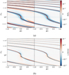 |
Fig. 1 r–ϕ maps of the density (a) and radial velocity (b) perturbation fields from the simulation (left panel) and analytical model (right panel) in the Mp = 0.25 mth case. The black dotted line represents the linear wake (Eq. (11)). The color bar is logarithmic above 0.01 km s−1 and linear below it. For reference, the Keplerian speed at the planet location is vK = 3 km s−1. |
3.1 Low mass limit
In this section, we present the results we obtained in the low planet mass limit (mp ≪ mth). In Fig. 1a, we compare the density perturbations extracted from the simulation against those computed using WAKEFLOW. The black dotted curve represents the spiral wake given by the linear approximation (Eq. (11)). In this regime, the pitch angle of the spirals is comparable; however, their amplitude and width are smaller in the analytic model. Moreover, the simulation shows the presence of an additional positive spiral arm below the black dotted line.
We show the same comparison for the radial velocity field in Fig. 1b. In this case, the width and amplitude differences are less severe compared to the density perturbation. The analytic model features a discontinuity between the linear and non-linear regions. This is because both the density and radial velocity in the linear regime are taken from the simulation, while only the density was obtained solving Burgers’ equation in the non-linear regime. The velocity components were then computed using Eqs. (23)–(24), which are obtained from Eqs. (2)–(3), neglecting higher order terms (Rafikov 2002). We believe this simplification in the model to be the source of the discontinuity.
We compared the properties of the spiral more quantitatively by looking at the azimuthal (η) profiles of the density and radial velocity perturbations, shown in Figs. 2a and 2b, respectively. The density profiles exhibit features similar to the ones presented in Cimerman & Rafikov (2021). When compared with the simulation, the amplitude of the spiral computed from Burgers’ equation suffers a stronger decay, and the shocks advance more slowly in the azimuthal direction. Moreover, the analytic profiles feature steep shock fronts, in contrast with the smoother profiles from the simulation, which are due to diffusive effects introduced by viscosity. Viscous diffusion affects the perturbations by lowering their amplitude while increasing their azimuthal extent. Indeed, the simulated profiles are wider than the analytic ones, but they still feature a higher amplitude. This suggests that the analytic model tends to overestimate the wave damping, in agreement with the results found in Cimerman & Rafikov (2021).
While we note that using a simulation with very low viscosity (α ≪ 10−4) would provide an ideal comparison with the inviscid analytic model, we have noticed that setting such a low α parameter triggers the onset of numerical effects, requiring an even higher resolution in order to remove them. Although increasing viscosity up to α = 10−3 removes these numerical artifacts, it also causes strong diffusion and makes a direct comparison between the simulated and analytic profiles more complicated. We find that choosing α = 10−4 gives the best trade off between suppressing numerical effects and limiting viscous spreading. However, we still see the presence of small oscillations at the shock fronts. In Appendix A, we use the α = 10−3 simulations to check that these oscillations are a result of the low viscosity and that they do not affect our results.
Additionally, we observed the presence of a positive peak for negative η in the simulation. This affects both the amplitude and width of the profile, causing the strongest deviation between the simulation and the model. Although the velocity profiles are remarkably different close to the planet due to the discontinuity previously discussed, after about 0.2 rp their behaviour becomes very similar to that of the density perturbations.
Lastly, we can define the centre of the spiral as the point where the perturbations change sign but only when the wave-fronts have already undergone a shock and the spiral features its characteristic N shape. This point is fixed by construction in the analytic model. We note that this is not the case in the simulation, where the centre of the spiral features a positive azimuthal shift. This implies that the pitch angle of the spiral from the analytical model is different with respect to that of the simulation at the centre of the spiral.
3.2 Intermediate mass limit
Next, we consider the results we obtain when the planet mass approaches the thermal mass. The main assumption of the semi-analytical model we are testing is that the perturbations are linear close to the planet. This is equivalent to the requirement mp < 1 mth. We tested this limit to assess the validity of the model when the linear assumption is not satisfied.
By comparing Figs. 3a, b with Figs. 1a, b, we observed that the planet starts to carve a gap in the disc. The density perturbations show positive features at the edge of the gap in the co-orbital region, while the velocity shows material rotating around the planet position. In this limit, the spiral becomes wider and stronger, as expected for a more massive planet. Although the amplitude of the perturbations now holds a better comparison between the simulation and the model, the discrepancy in pitch angle and width of the spiral increases. This is more evident in Figs. 4a, b. The general features shown by the profiles are similar to the low mass case, with the exception of their width. In this case, the analytic profiles are wider than the simulation, where the centre of the spiral suffers a stronger azimuthal shift.
In Fig. 5, we compare the azimuthal position of the minimum (yellow) and maximum (blue) of the density profiles with respect to the linear wake (black dashed line). We observed that the deviation between the simulation (solid lines) and the analytic model (dash-dotted lines) for the maximum increases up to 0.25 radians and remains stationary after 2.0 r/rp. On the other hand, the deviation for the minimum has an oscillatory behaviour until 1.8 r/rp, after which it starts increasing until the outer edge of the disc, reaching a value of 1.00 radians. This asymmetry not only changes the width of the profile, affecting the planet mass estimate3, but it also results in a shift in pitch angle. The deviation of the pitch angle for spirals induced by massive planets from the linear prediction was also reported in the simulations of Zhu et al. (2015); Bae & Zhu (2018). In the figure, we have also plotted the non-linear correction from Eq. (13) (black dot dashed line) that was introduced in Cimerman & Rafikov (2021) to correct this behaviour. Although this non-linear correction is valid for planet masses below the thermal limit, it deviates considerably from the peak of both the simulation and the analytical model above this limit. Thus the correction needs to be revisited in the limit of intermediate and high planet masses (mp≥ mth).
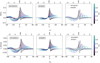 |
Fig. 2 Comparison between simulated (left) and analytical (middle) density (a) and radial velocity (b) η (azimuthal) profiles in the outer disc for the Mp = 0.25 mth case. In the right panels, we show a choice of profiles from the simulation (solid line) and the analytic model (dash dotted line) to better highlight the differences in individual profiles. The color scale shows the radial distance from the planet. We filtered the profiles from the simulation using the savgol_filter function from the scipy Python library to reduce the oscillations at the shock fronts (see Appendix A). |
3.3 Observational applications
Kinematic observations of protoplanetary discs have shown the presence of complex structures that can be associated with planet candidates (Pinte et al. 2020; Izquierdo et al. 2023). To visually test the applicability of the semi-analytical model to observations, we coupled WAKEFLOW with DISCMINER (Izquierdo et al. 2021). The latter fits each channel map with a parametric model describing physical and geometrical properties of the disc. It is possible to use a single or double Gaussian or a Bell line profile model at each pixel, enabling differentiation between the emission from the upper and lower surfaces of the disc. The DISCMINER model assumes a Keplerian axisymmetric velocity field. In this way, it can minimise the residuals between the observations and the model in order to fit for the disc parameters, but it cannot predict planet properties such as the planet mass.
We can model the presence of a planet by adding the velocity field computed with WAKEFLOW on top of the background Keplerian field of DISCMINER. Once we computed the perturbed field using our semi-analytical model, we could produce channel maps to perform a direct comparison with observed data. In a similar way, we can produce channel maps using the velocity field from the simulation.
Figure 6 presents the DISCMINER channel maps we produced using the simulation (top row) and WAKEFLOW (middle row) velocity field. In the bottom row, we also show the residuals between the two models. We show the output for a planet with mp = 1 mth in a disc with hp/rp = 0.05 (left column) and hp/rp = 0.1 (right column), respectively. This is equivalent to having a planet with mp ≃ 0.09 MJ and mp ≃ 0.7 MJ. We note how the perturbations in the first case have a very low amplitude are thus barely noticeable compared to the disc with a more realistic disc aspect ratio. This is because the kink amplitude ![$\[\mathcal{A}\]$](/articles/aa/full_html/2024/07/aa50087-24/aa50087-24-eq27.png) , defined as the maximum deviation from the unperturbed channel map, scales as
, defined as the maximum deviation from the unperturbed channel map, scales as ![$\[\mathcal{A}\]$](/articles/aa/full_html/2024/07/aa50087-24/aa50087-24-eq28.png) ∝ mp1/2 (Bollati et al. 2021), so the low planet mass excites perturbations with an amplitude of ~1% of the Keplerian velocity at the planet location. This does not change the behaviour of the model in the different regimes compared to the thermal mass, but it confirms how only planets in the Jupiter mass range or above can be detected with this method. The residuals in the bottom row highlight how the different pitch angle causes the spirals to cross the channel maps in different locations, producing oscillating residuals that do not cancel out, unlike when the amplitude of the spirals between the simulation and the model are comparable. As a result, a procedure that minimises this type of residuals cannot be used to estimate planet masses.
∝ mp1/2 (Bollati et al. 2021), so the low planet mass excites perturbations with an amplitude of ~1% of the Keplerian velocity at the planet location. This does not change the behaviour of the model in the different regimes compared to the thermal mass, but it confirms how only planets in the Jupiter mass range or above can be detected with this method. The residuals in the bottom row highlight how the different pitch angle causes the spirals to cross the channel maps in different locations, producing oscillating residuals that do not cancel out, unlike when the amplitude of the spirals between the simulation and the model are comparable. As a result, a procedure that minimises this type of residuals cannot be used to estimate planet masses.
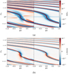 |
Fig. 3 r–ϕ map of the density (a) and radial velocity (b) perturbation fields from the simulation (left panel) and analytical model (right panel) in the Mp = 1.00 mth case. The black dotted line represents the linear wake (Eq. (11)). The color bar is logarithmic above 0.01 km s−1 and linear below it. For reference, the Keplerian speed at the planet location is vK = 3 km s−1. |
3.4 Limitations of this work
In the previous sections, we focused our analysis on the comparison between 2D hydrodynamical simulations with a globally isothermal equation of state and our analytic model in order to test this framework using models sharing the same assumptions. However, real protoplanetary discs have a 3D structure and may feature cooling processes, likely resulting in vertical thermal stratification. Both the vertical structure of the disc (Zhu et al. 2015; Pinte et al. 2019; Rosotti et al. 2020; Rabago & Zhu 2021) and more realistic thermodynamics prescriptions (Miranda & Rafikov 2019, 2020; Ziampras et al. 2023) change the spiral structure generated by a planet, thus affecting planet mass estimates obtained from the analysis of its morphology.
Muley et al. (2024) have recently performed 3D hydrodynamical simulations comparing different thermodynamic prescriptions, from locally isothermal to β-cooling and three-temperature radiation hydrodynamics. They studied the density and radial velocity azimuthal profiles at the midplane and at the emitting layer of 12CO for their different thermodynamic prescriptions and have found that using more realistic equations of state produces perturbations in the midplane with lower amplitudes compared with the locally isothermal case. Above the midplane, all the prescriptions instead produce radial velocity perturbations with approximately the same amplitude, which is lower compared to the isothermal case in the midplane. As the planet mass is directly related to the amplitude of the perturbations (Bollati et al. 2021; Rabago & Zhu 2021) and the analytical framework assumes that the emission comes from the midplane of a globally isothermal disc, we then expected that applying the analytical model to spirals coming from a finite height in a vertically temperature-stratified disc will produce lower planet mass estimates.
Additionally, numerical 3D simulations have shown that planetary spirals are less tightly wound in the upper layers of the disc (Zhu et al. 2015; Rosotti et al. 2020), due to the vertical temperature gradient of the disc. Following our discussion in Sect. 3.3, constraining the pitch angle dependence on the disc parameters also in the vertical direction is crucial to performing a fitting procedure using the analytical framework and to obtaining accurate estimates of planet masses.
4 Conclusions
The focus of the search for protoplanets is moving towards kinematic detections. With the development of new techniques to reveal protoplanet candidates, new possibilities are opening for the characterisation of their properties. Together with incoming observational constraints, novel and improved models need to be developed and robustly tested. In this paper, we have numerically tested the semi-analytical model for planet-induced spiral waves introduced in Bollati et al. (2021) with a set of 2D FARGO3D simulations in the low (< 1 mth) and intermediate (~1 mth) planet mass regime. In contrast to previous studies in the low planet mass regime (Cimerman & Rafikov 2021), our analysis was aimed at assessing the applicability of this analytical model to observations by testing the velocity field in the intermediate mass regime, as this is the quantity directly detected by kinematic observations. The results we obtained can be summarised as follows:
The comparison with the simulation with a 0.25 mth planet shows similar results with those obtained in Cimerman & Rafikov (2021) for the density field. Although qualitatively similar, the solution of Burgers’ equation propagates faster with respect to the simulations, producing spirals with a smaller width and amplitude. We found the same behaviour for the radial velocity component for a radial distance greater than ~0.2 r/rp from the planet.
Both perturbations feature a positive azimuthal shift in the centre of the spiral and a secondary spiral arm in the simulations, which are not present in the analytical model. This produces a change in pitch angle, even for low planet masses.
The velocity field computed from the semi-analytical model features a discontinuity at the interface between the linear and non-linear regions. This discontinuity is present in both planetary regimes.
For the simulation with a 1 mth planet, the discrepancy increases. The model produces profiles with a smaller amplitude but larger width, and it fails to reproduce the shift in azimuth present in the simulation profiles. This results in a different pitch angle. Moreover, the correction introduced in Cimerman & Rafikov (2021) does not reproduce the expected pitch angle from the simulation in this limit.
Although the general behaviour of the model is in good qualitative agreement with the simulation, the difference in pitch angle causes the two spirals to not overlap. As a result, standard fitting procedures based on the minimisation of residuals cannot converge. In order to apply this model to observations, it is necessary to revisit it while accounting for the shift in pitch angle and the discontinuity in the velocity field that are present for all planet masses. An alternative approach for fitting planet masses would consist of developing a parametric model for the velocity perturbations. Exploring these possibilities will be the scope of future work.
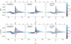 |
Fig. 4 Comparison between simulated (left) and analytical (middle) density (a) and radial velocity (b) η (azimuthal) profiles in the outer disc for the Mp = 1.00 mth case. In the right panels, we show a choice of profiles from the simulation (solid line) and the analytic model (dash dotted line) to better highlight the differences in individual profiles. The color scale shows the radial distance from the planet. We filtered the profiles from the simulation using the savgol_filter function from the scipy Python library to reduce the oscillations at the shock fronts (see Appendix A). |
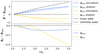 |
Fig. 5 Azimuthal deviation of the pitch angle from the linear prediction. Top panel: azimuthal distance of the maximum (blue) and minimum (yellow) from the linear wake prediction for the Mp = 1.00 mth case. We used this estimate to trace the pitch angle of the spiral wake. Solid lines represent the values obtained from the simulation, while dash dotted lines are obtained from the analytical model. Bottom panel: difference between the maximum (blue) and minimum (yellow) from the analytical model and the simulation as a function of the disc radius. |
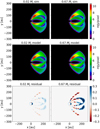 |
Fig. 6 Expected kink in the channel maps for a thermal mass planet in a disc with hp/rp = 0.05 (left column) and hp/rp = 0.1 (right column), resulting in a planet mass of mp ≃ 0.02 MJ and mp ≃ 0.67 MJ, respectively. We arbitrarily set the inclination of the disc to i = −45°. Top row: channel maps obtained from the velocity field of the simulation. Middle row: channel maps obtained from the velocity field of the analytical model. Bottom row: intensity residuals between the channel maps obtained from the velocity field of the simulation and the analytic model. |
Acknowledgements
We thank the referee for the constructive feedback provided that helped improve the manuscript. We also thank Jochen Stadler, Bin Ren and Enrico Ragusa for the useful discussions. This project has received funding from the European Research Council (ERC) under the European Union’s Horizon 2020 research and innovation programme (PROTOPLANETS, grant agreement no. 101002188). This work has received funding from the European Union’s Horizon 2020 research and innovation programme under the Marie Sklodowska-Curie grant agreement no. 823823 (RISE DUSTBUSTERS project). A.J.W. has received funding from the European Union’s Horizon 2020 research and innovation programme under the Marie Skłodowska-Curie grant agreement no. 101104656. GR and AR acknowledge support from the European Union (ERC Starting Grant DiscEvol, project number 101039651) and from Fondazione Cariplo, grant no. 2022-1217. Views and opinions expressed are, however, those of the author(s) only and do not necessarily reflect those of the European Union or the European Research Council. Neither the European Union nor the granting authority can be held responsible for them. Computational resources have been provided by INDACO Core facility, which is a project of High Performance Computing at the Universitá degli Studi di Milano (https://www.unimi.it). Support for AI was provided by NASA through the NASA Hubble Fellowship grant no. HST-HF2-51532.001-A awarded by the Space Telescope Science Institute, which is operated by the Association of Universities for Research in Astronomy, Inc., for NASA, under contract NAS5-26555.
Appendix A High viscosity simulation
In Fig. A.1b, we show the third panel of Fig. 2b and compare it with the same result obtained using simulations with α = 0 and α = 10−3 (Fig. A.1c). In this appendix, we show the full extent of the oscillations, whereas in the main text we filter them using the savgol_filter function from the scipy Python library. While the profiles from the lower viscosity simulation are completely dominated by oscillations, the higher viscosity simulation does not show any sign of them. These oscillations are likely due to numerical instabilities and are damped out with increasing viscosity. However the viscous damping of the profiles becomes too strong for α = 10−3, especially far away from the planet position, making a direct comparison between the analytical model and the simulations more challenging. As the structure of the perturbations is otherwise unchanged, we could safely carry out our analysis on the simulations with α = 10−4.
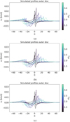 |
Fig. A.1 Comparison of a choice of radial velocity azimuthal profiles from the simulation (solid line) and the analytic model (dash dotted line) using α = 0 (a), α = 10−4 (b), and α = 10−3 (c). |
References
- Andrews, S. M., Huang, J., Pérez, L. M., et al. 2018, ApJ, 869, L41 [NASA ADS] [CrossRef] [Google Scholar]
- Armitage, P. J. 2015, arXiv e-prints [arXiv:1509.06382] [Google Scholar]
- Bae, J., & Zhu, Z. 2018, ApJ, 859, 118 [Google Scholar]
- Bae, J., Isella, A., Zhu, Z., et al. 2023, in ASP Conf. Ser., 534, Protostars and Planets VII, eds. S. Inutsuka, Y. Aikawa, T. Muto, K. Tomida, & M. Tamura, 423 [Google Scholar]
- Benítez-Llambay, P., & Masset, F. S. 2016, ApJS, 223, 11 [Google Scholar]
- Bollati, F., Lodato, G., Price, D. J., & Pinte, C. 2021, MNRAS, 504, 5444 [Google Scholar]
- Cimerman, N. P., & Rafikov, R. R. 2021, MNRAS, 508, 2329 [NASA ADS] [CrossRef] [Google Scholar]
- Disk Dynamics Collaboration (Armitage, P. J., et al.) 2020, arXiv e-prints [arXiv:2009.04345] [Google Scholar]
- Flock, M., Ruge, J. P., Dzyurkevich, N., et al. 2015, A&A, 574, A68 [NASA ADS] [CrossRef] [EDP Sciences] [Google Scholar]
- Goldreich, P., & Tremaine, S. 1979, ApJ, 233, 857 [Google Scholar]
- Goldreich, P., & Tremaine, S. 1980, ApJ, 241, 425 [Google Scholar]
- Goodman, J., & Rafikov, R. R. 2001, ApJ, 552, 793 [NASA ADS] [CrossRef] [Google Scholar]
- Hilder, T., Fasano, D., Bollati, F., & Vandenberg, J. 2023, J. Open Source Softw., 8, 4863 [CrossRef] [Google Scholar]
- Izquierdo, A. F., Testi, L., Facchini, S., Rosotti, G. P., & van Dishoeck, E. F. 2021, A&A, 650, A179 [NASA ADS] [CrossRef] [EDP Sciences] [Google Scholar]
- Izquierdo, A. F., Testi, L., Facchini, S., et al. 2023, A&A, 674, A113 [NASA ADS] [CrossRef] [EDP Sciences] [Google Scholar]
- Lodato, G., Dipierro, G., Ragusa, E., et al. 2019, MNRAS, 486, 453 [Google Scholar]
- Masset, F. 2000, A&ASS, 141, 165 [NASA ADS] [CrossRef] [EDP Sciences] [Google Scholar]
- Miranda, R., & Rafikov, R. R. 2019, ApJ, 875, 37 [Google Scholar]
- Miranda, R., & Rafikov, R. R. 2020, ApJ, 892, 65 [NASA ADS] [CrossRef] [Google Scholar]
- Muley, D., Melon Fuksman, J. D., & Klahr, H. 2024, A&A, 687, A213 [NASA ADS] [CrossRef] [EDP Sciences] [Google Scholar]
- Ogilvie, G. I., & Lubow, S. H. 2002, MNRAS, 330, 950 [Google Scholar]
- Okuzumi, S., Tanaka, H., Kobayashi, H., & Wada, K. 2012, ApJ, 752, 106 [NASA ADS] [CrossRef] [Google Scholar]
- Papaloizou, J., & Lin, D. N. C. 1984, ApJ, 285, 818 [NASA ADS] [CrossRef] [Google Scholar]
- Perez, S., Dunhill, A., Casassus, S., et al. 2015, ApJ, 811, L5 [NASA ADS] [CrossRef] [Google Scholar]
- Pérez, S., Casassus, S., & Benítez-Llambay, P. 2018, MNRAS, 480, L12 [Google Scholar]
- Pinte, C., Price, D. J., Ménard, F., et al. 2018, ApJ, 860, L13 [Google Scholar]
- Pinte, C., van der Plas, G., Ménard, F., et al. 2019, Nat. Astron., 3, 1109 [NASA ADS] [CrossRef] [Google Scholar]
- Pinte, C., Price, D. J., Ménard, F., et al. 2020, ApJ, 890, L9 [CrossRef] [Google Scholar]
- Pinte, C., Teague, R., Flaherty, K., et al. 2023, in ASP Conf. Ser., 534, Protostars and Planets VII, eds. S. Inutsuka, Y. Aikawa, T. Muto, K. Tomida, & M. Tamura, 645 [Google Scholar]
- Rabago, I., & Zhu, Z. 2021, MNRAS, 502, 5325 [NASA ADS] [CrossRef] [Google Scholar]
- Rafikov, R. R. 2002, ApJ, 569, 997 [Google Scholar]
- Rosotti, G. P., Benisty, M., Juhász, A., et al. 2020, MNRAS, 491, 1335 [Google Scholar]
- Shakura, N. I., & Sunyaev, R. A. 1973, A&A, 24, 337 [NASA ADS] [Google Scholar]
- Teague, R., Bae, J., Bergin, E. A., Birnstiel, T., & Foreman-Mackey, D. 2018, ApJ, 860, L12 [NASA ADS] [CrossRef] [Google Scholar]
- Val-Borro, M. D., Edgar, R. G., Artymowicz, P., et al. 2006, MNRAS, 370, 529 [NASA ADS] [CrossRef] [Google Scholar]
- Zhu, Z., Dong, R., Stone, J. M., & Rafikov, R. R. 2015, ApJ, 813, 88 [Google Scholar]
- Ziampras, A., Nelson, R. P., & Rafikov, R. R. 2023, MNRAS, 524, 3930 [NASA ADS] [CrossRef] [Google Scholar]
The azimuthal width of the profiles scales with the planet mass as ![$\[m_{\mathrm{p}}^{1 / 2}\]$](/articles/aa/full_html/2024/07/aa50087-24/aa50087-24-eq29.png) (Bollati et al. 2021).
(Bollati et al. 2021).
All Tables
All Figures
|
Fig. 1 r–ϕ maps of the density (a) and radial velocity (b) perturbation fields from the simulation (left panel) and analytical model (right panel) in the Mp = 0.25 mth case. The black dotted line represents the linear wake (Eq. (11)). The color bar is logarithmic above 0.01 km s−1 and linear below it. For reference, the Keplerian speed at the planet location is vK = 3 km s−1. |
| In the text | |
|
Fig. 2 Comparison between simulated (left) and analytical (middle) density (a) and radial velocity (b) η (azimuthal) profiles in the outer disc for the Mp = 0.25 mth case. In the right panels, we show a choice of profiles from the simulation (solid line) and the analytic model (dash dotted line) to better highlight the differences in individual profiles. The color scale shows the radial distance from the planet. We filtered the profiles from the simulation using the savgol_filter function from the scipy Python library to reduce the oscillations at the shock fronts (see Appendix A). |
| In the text | |
|
Fig. 3 r–ϕ map of the density (a) and radial velocity (b) perturbation fields from the simulation (left panel) and analytical model (right panel) in the Mp = 1.00 mth case. The black dotted line represents the linear wake (Eq. (11)). The color bar is logarithmic above 0.01 km s−1 and linear below it. For reference, the Keplerian speed at the planet location is vK = 3 km s−1. |
| In the text | |
|
Fig. 4 Comparison between simulated (left) and analytical (middle) density (a) and radial velocity (b) η (azimuthal) profiles in the outer disc for the Mp = 1.00 mth case. In the right panels, we show a choice of profiles from the simulation (solid line) and the analytic model (dash dotted line) to better highlight the differences in individual profiles. The color scale shows the radial distance from the planet. We filtered the profiles from the simulation using the savgol_filter function from the scipy Python library to reduce the oscillations at the shock fronts (see Appendix A). |
| In the text | |
|
Fig. 5 Azimuthal deviation of the pitch angle from the linear prediction. Top panel: azimuthal distance of the maximum (blue) and minimum (yellow) from the linear wake prediction for the Mp = 1.00 mth case. We used this estimate to trace the pitch angle of the spiral wake. Solid lines represent the values obtained from the simulation, while dash dotted lines are obtained from the analytical model. Bottom panel: difference between the maximum (blue) and minimum (yellow) from the analytical model and the simulation as a function of the disc radius. |
| In the text | |
|
Fig. 6 Expected kink in the channel maps for a thermal mass planet in a disc with hp/rp = 0.05 (left column) and hp/rp = 0.1 (right column), resulting in a planet mass of mp ≃ 0.02 MJ and mp ≃ 0.67 MJ, respectively. We arbitrarily set the inclination of the disc to i = −45°. Top row: channel maps obtained from the velocity field of the simulation. Middle row: channel maps obtained from the velocity field of the analytical model. Bottom row: intensity residuals between the channel maps obtained from the velocity field of the simulation and the analytic model. |
| In the text | |
|
Fig. A.1 Comparison of a choice of radial velocity azimuthal profiles from the simulation (solid line) and the analytic model (dash dotted line) using α = 0 (a), α = 10−4 (b), and α = 10−3 (c). |
| In the text | |
Current usage metrics show cumulative count of Article Views (full-text article views including HTML views, PDF and ePub downloads, according to the available data) and Abstracts Views on Vision4Press platform.
Data correspond to usage on the plateform after 2015. The current usage metrics is available 48-96 hours after online publication and is updated daily on week days.
Initial download of the metrics may take a while.