| Issue |
A&A
Volume 687, July 2024
|
|
|---|---|---|
| Article Number | A18 | |
| Number of page(s) | 8 | |
| Section | Interstellar and circumstellar matter | |
| DOI | https://doi.org/10.1051/0004-6361/202449824 | |
| Published online | 25 June 2024 | |
Magnetic field dragging in filamentary molecular clouds
1
Dipartimento di Fisica e Astronomia, Università degli Studi di Firenze,
Italy
e-mail: domitilla.tapinassi@edu.unifi.it
2
INAF – Osservatorio Astrofisico di Arcetri,
Largo E. Fermi 5,
50125
Firenze, Italy
e-mail: daniele.galli@inaf.it
3
Max Planck Institute for Astronomy,
Königstuhl 17,
69117
Heidelberg, Germany
Received:
1
March
2024
Accepted:
15
May
2024
Context. Maps of polarized dust emission of molecular clouds reveal the morphology of the magnetic field associated with star-forming regions. In particular, polarization maps of hub-filament systems show the distortion of magnetic field lines induced by gas flows onto and inside filaments.
Aims. We aim to understand the relation between the curvature of magnetic field lines associated with filaments in hub-filament systems and the properties of the underlying gas flows.
Methods. We consider steady-state models of gas with finite electrical resistivity flowing across a transverse magnetic field. We derive the relation between the bending of the field lines and the flow parameters represented by the Alfvén Mach number and the magnetic Reynolds number.
Results. We find that, on the scale of the filaments, the relevant parameter for a gas of finite electrical resistivity is the magnetic Reynolds number, and we derive the relation between the deflection angle of the field from the initial direction (assumed perpendicular to the filament) and the value of the electrical resistivity, due to either Ohmic dissipation or ambipolar diffusion.
Conclusions. Application of this model to specific observations of polarized dust emission in filamentary clouds shows that magnetic Reynolds numbers of a few tens are required to reproduce the data. Despite significant uncertainties in the observations (the flow speed, the geometry and orientation of the filament), and the idealization of the model, the specific cases considered show that ambipolar diffusion can provide the resistivity needed to maintain a steady state flow across magnetic fields of significant strength over realistic time scales.
Key words: ISM: clouds / dust, extinction / ISM: kinematics and dynamics / ISM: magnetic fields
© The Authors 2024
 Open Access article, published by EDP Sciences, under the terms of the Creative Commons Attribution License (https://creativecommons.org/licenses/by/4.0), which permits unrestricted use, distribution, and reproduction in any medium, provided the original work is properly cited.
This article is published in open access under the Subscribe to Open model. Subscribe to A&A to support open access publication.
1 Introduction
The filamentary structure of molecular clouds has recently received significant attention, both observationally and theoretically, particularly in relation to the morphology of the associated magnetic field derived from optical, near-infrared and submillimeter polarization maps (see, e.g., Pattle et al. 2023, for a recent review). Various theoretical models have been developed to describe self-gravitating cylindrical filaments in hydrostatic equilibrium, partially supported by magnetic fields with a poloidal, toroidal or helical geometry (Nagasawa 1987; Fiege & Pudritz 2000; Tomisaka 2014; Toci & Galli 2015a,b). While these characteristics may be suitable for describing massive and relatively isolated filaments, a frequently observed feature in star-forming regions is the “hub-filament” structure, consisting of a network of filaments converging to a central density concentration (the “hub”) hosting star and cluster formation (see, e.g., Myers 2009).
Velocity gradients observed along filaments (see, e.g., Friesen et al. 2013; Kirk et al. 2013; Pan et al. 2024) suggest the presence of accretion flows possibly driven by the gravitational attraction of dense clumps or hubs. This is also supported by numerical simulations (Zamora-Avilés et al. 2017; Gómez et al. 2018). However, these velocity gradients can also be interpreted as projection of large-scale turbulence (Fernández-López et al. 2014). lf these accretion flows exist, they would be responsible for feeding star formation in the central hub, and for dragging the magnetic field lines, stretching and progressively aligning them with the filament’s axis (Juárez et al. 2017; Yuan et al. 2018; Wang et al. 2020; Koch et al. 2022).
In some high-mass star-forming regions the overall morphology of the hub-filament system takes the form of a spiral pattern, which could be the consequence of a coherent large-scale rotation motion in the parent clump (Li et al. 2017; Liu et al. 2018; Schwörer et al. 2019; Mookerjea et al. 2023). When available, the direction of polarized dust emission in these regions generally follows the spiral pattern, indicating that the magnetic field morphology is primarily shaped by the gas dynamics. Some examples of such regions include the high-mass star-forming complexes Monoceros R2 (Treviño-Morales et al. 2019), G9.62+0.19 (Dall’Olio et al. 2019), G327.3 (Beuther et al. 2020), lRAS 18089-1732 (Sanhueza et al. 2021), and Monoceros R2 (Hwang et al. 2022).
In other cases of hub-filament systems there appears to be a progressive transition in the orientation of the magnetic field. The field is preferentially parallel to relatively low column density filaments (also known as “striations”), but, as column density increases, it becomes preferentially perpendicular to filaments (see, e.g., Chapman et al. 2011; Cox et al. 2016; Arzoumanian et al. 2021; Chen et al. 2023). This change occurs at a visual extinction of AV ≈ 2.7 mag, corresponding to a column density of NH ≈ 1021.7 cm−2 (Planck Collaboration Int. XXXV 2016). ln this scenario, the magnetic field within a filament is stretched in the longitudinal direction by the accretion flow, taking on a strongly pinched “hairpin”- or “U”-shape. Observations of bow- or U-shaped magnetic fields have been made in various regions, such as the massive infrared-dark cloud G035.39-00.33 (Liu et al. 2018), the high-mass star-forming region G327.3 (Beuther et al. 2020), and the massive hub-filament system SDC13 (Wang et al. 2022). ln all of these regions, it seems that the magnetic field has been partially dragged by the collapsing gas flows responsible for forming the densest structures. This scenario of dragged magnetic fields and accretion flows within filaments finds support in high-resolution and high-sensitivity observations of polarized dust emission. These observations have resolved the magnetic field structure inside filaments at scales <0.1 pc. ln some cases, they have revealed a transition from perpendicular to aligned fields occurring at AV ≈ 21 mag (NH ≈ 1022.6 cm−2) in the Serpens South molecular cloud (Pillai et al. 2020) and in the hub-filament system NGC 6334 (Arzoumanian et al. 2021).
In this work, we investigate the configuration of the magnetic field in and around a filament that results from dragging and bending a pre-existing uniform magnetic field by a prescribed accretion flow. Our motivation is to establish the relationship between observable geometrical characteristics of the field (as derived from dust polarization maps) and the physical properties of the filament. First, in Sect. 2 we consider the case of clumpy filaments, made by perfectly conducting localized overdensities that move toward the central hub across the cloud’s magnetic field. Then, in Sect. 3 we examine the configuration of the magnetic field in stationary accretion-diffusion flows with constant Ohmic or ambipolar diffusion resistivity. ln Sect. 4, we apply the methods described in Sects. 2–3 to two specific examples, the hub-filament structure in the Serpens South molecular cloud and the high-mass star-forming region G327.3, and derive the magnetic field strength from available dust polarization data. Finally, in Sect. 5 we discuss the implications of this work, and in Sect. 6 we draw our conclusions.
2 Alfvén wings
Gómez et al. (2018) explore the shape of magnetic field lines in MHD simulations, in which filaments are long-lived structures that channel gas flows toward a central accreting clump. Along the spines of these filaments, transverse magnetic field lines are stretched by the flow and assume a U-shape. The geometrical characteristics of this U-shape depend on the flow velocity, density and magnetic field strength. According to Gómez et al. (2018), the curvature of the field lines depends on the Alfvén Mach number MA = u/vA, defined as the ratio of the longitudinal flow speed u and the Alfvén speed  determined by the strength of the magnetic field B and the density ρ of the filament. Therefore, by analyzing the observed curvature of magnetic field lines (from maps of polarized dust emission) one could potentially determine the Alfvén Mach number of the flow.
The relation between the geometry of the magnetic field and flow properties has been extensively studied in the case of localized overdensities (clumps, or “bullets”) of density ρc and size a moving with speed u in a medium with density ρ < ρc across a transverse magnetic field (see, e.g., Lyutikov 2006; Dursi & Pfrommer 2008). The moving clump diverts the plasma on its sides and bends the ambient magnetic field into wedge-shaped structures similar to Cherenkov cones, called “Alfvén wings.” These wings are characterized by a deflection angle θ in the plane containing the flow direction and the background magnetic field, as given by

(Drell et al. 1965; Neubauer 1980). The formation of Alfvén wings has been investigated in the context of satellites moving in the magnetospheric plasma of a planet (Kivelson et al. 2007), planets interacting with the solar wind (Baumjohann et al. 2010), and galaxy clusters moving in the magnetized intracluster medium (Lyutikov 2006). Equation (1) has been validated through numerical simulations (see, e.g., Linker et al. 1991; Dursi & Pfrommer 2008). When MA is sufficiently large, the wings can fold over the moving clump to form a magnetotail.
This scenario is valid if the electrical resistivity of the clump is low enough that the time scale of magnetic diffusion across the scale a is much longer than its crossing time a/u, and the clump can be considered a perfect conductor. In this case, the ambient magnetic field is swept up and accumulates in a strongly magnetized boundary layer of thickness approximately equal to  ahead of the clump, where magnetic tension approximately balances the ram pressure gradient (Gómez et al. 2018). At this point the magnetic tension of the stretched and compressed field acts essentially as a hydrodynamical drag, decelerating the clump on a braking time scale tbr ≈ δa/u, where δ = ρc/ρ > 1 (Dursi & Pfrommer 2008). This is the well-known expression for the braking time of an aligned rotator of density ρc in an external medium with density ρ (Ebert et al. 1960; Mouschovias 1977), with the Alfvén speed in the “external medium” (the boundary layer) replaced by the clump’s speed u by virtue of the balance of magnetic and ram pressure. Actually, if the clump is moving at supersonic speed, internal shocks propagating at speed us = u/δ1/2 promote instabilities that disrupt the clump in a time approximately equal to a/us = δ1/2a/u, shorter than tbr by a factor δ1/2 (see, e.g., Jones et al. 1994, 1996).
As recognized by Gómez et al. (2018), in order for gas to flow longitudinally along a filament across a transverse magnetic field, some of magnetic diffusion must be involved. Without it, a fluid element of size a would only be able to travel a distance approximately equal to δa or δ1/2a before being stopped by magnetic tension or disrupted by internal shocks. Additionally, Eq. (1) suggests that large deflection angles, greater than 45°, for example, are a result of motions at super-Alfvénic speeds. Although the determination of MA in filament-hub system is uncertain, current observations based on the interpretation of sub-mm dust polarization maps and molecular line emission indicate that, generally, MA ≲ 1 in filaments, and MA ≳ 1 only in or near the central clump/hub (Beltrán et al. 2019, 2024; Hwang et al. 2022). In the next section we examine the effects of a finite electrical resistivity on the motion of gas in a filament across a transverse magnetic field.
3 Magnetic diffusion
A finite electrical resistivity η substantially modifies the situation described in Sect. 2. Instead of accumulating in front of the moving clump, the ambient magnetic field can pass through the fluid more or less unimpeded, depending on the value of the magnetic Reynolds number

which represents the ratio of diffusion time scale a2/η to the crossing time a/u. In the presence of magnetic diffusion, the effect of flow on the geometry of the magnetic field is no longer described by the Alfvén Mach number, but by the magnetic Reynolds number. This situation can be illustrated by the following example: consider an electrically conducting fluid with a constant density ρ and Ohmic resistivity η, flowing with a velocity u in the x-direction, perpendicular to a magnetic field B in the z-direction (see Fig. 1). The fluid motion induces an electric current in the y-direction given by Ohm’s law as j = ucB/(4πη), where c is the speed of light1. The Lorentz force per unit mass is then F = jB/(cρ) = uB2/(4πρη), directed opposite to the fluid motion. Therefore, the magnetic field exerts a drag on the fluid with a magnetic damping time  (see, e.g., Roberts 1967; Davidson 2001). The kinetic energy per unit volume is dissipated by Joule heating at a rate d(pu2/2)/dt = 4πη j2/c2 = ρu2/td. A steady flow can be maintained provided an external driving force is acting on the fluid on a time scale longer than td. Alfvénic disturbances generated within the flow propagate on a scale aS before being damped by magnetic diffusion, where S = R/MA is the Lundquist number.
Inspired by Gómez et al. (2018), in the following section we consider a steady flow along a filament. This flow is driven by some unspecified external cause such as gravity, shocks, large-scale turbulence, etc. Our goal is to compute the curvature of a magnetic field initially perpendicular to the flow. We assume a stationary state and neglect the back-reaction of the field on the fluid motion. In other words, we adopt a kinematic approximation (Parker 1963), which is the first step in a fully magnetohydrodynamical treatment. Unlike the situation considered in Sect. 2, no magnetized boundary layer is formed in this case. The fundamental parameter in this case is the magnetic Reynolds number, rather than the Alfvén Mach number.
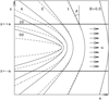 |
Fig. 1 Steady-state magnetic field lines for a flow with uniform resistivity and uniform velocity u (arrows) in a transverse magnetic field. for different values of the magnetic Reynolds number: R = 0.5, 1, 2, 4, 10 and 50. Solid lines: with ambipolar diffusion (R = Rad); dashed lines: with Ohmic resistivity (R = RO). The flow is limited to the region −a < z < a. The deflection angle θ is also shown. |
3.1 Diffusion-dominated gas flows
Let us consider an electrically resistive fluid flowing in the x-direction with velocity u between the planes z = ±a, while acting upon an initially uniform and perpendicular magnetic field B0 in the z-direction (see Fig. 1). The velocity u is assumed to vary on the scale of the filament’s length, which is much larger than the filament’s width. Therefore, it can be considered uniform over a region of size ~a. Magnetic field lines within the flow region will be stretched, progressively increasing their curvature until they eventually reach a state where field diffusion balances field advection, preventing any further increase in magnetic tension.
Let us first consider the case of a uniform Ohmic resistivity ηO. In this case, the induction equation is linear in the magnetic field, and can be “uncurled”2 into

where  .
.
With the non-dimensionalization z = aζ and Bx(z) = B0b(ζ) Eq. (3) becomes

where RO = au/ηO is the Ohmic magnetic Reynolds number. The solution of Eq. (4), with the symmetry boundary condition b(0) = 0 is

As anticipated, the motion of the resistive fluid in the perpendicular magnetic field has induced an electric current in the y-direction and a magnetic field Bx(z) = –R0B0z/a in the direction of the flow, leaving unchanged the magnetic field Bz = B0 perpendicular to the flow. Field lines are parabolas for |z| < a and straight lines for |z| > a. The deflection angle of the field lines for |z| > a is equal to the magnetic Reynolds number,

The evolution of the magnetic field toward this asymptotic steady state was computed by Lundquist (1952).
However, in the context of molecular clouds the magnetic Reynolds number RO is not relevant: Ohmic resistivity is negligible, and the electrical resistivity is dominated by ambipolar diffusion (see, e.g., Pinto et al. 2008; Gutiérrez-Vera et al. 2023). Although ambipolar diffusion introduces a non-linearity in the problem, a calculation of the asymptotic configuration of the field is straightforward. The uncurled induction equation is now
![${\bf{u}} \times {\bf{B}} + {{{\bf{B}} \times [{\bf{B}} \times (\nabla \times {\bf{B}})]} \over {4\pi \gamma {\rho _i}\rho }} = 0,$](/articles/aa/full_html/2024/07/aa49824-24/aa49824-24-eq11.png)
where γ is the ion-neutral drag coefficient and ρi the ion density. Equation (7) can be non-dimensionalized as before, obtaining

where Rad = au/ηad is the ambipolar diffusion magnetic Reynolds number, with ambipolar diffusion resistivity

assumed constant in the following. By interchanging the dependent and independent variables, Eq. (8) can be easily integrated with the boundary condition ζ(b = 0) = 0, resulting in
 (10)
(10)
The solution for b(ζ) is then
 (11)
(11)
where α = Radζ. For |z| > a, fieldlines are bent back from the direction perpendicular to the flow by an angle θ given by
 (12)
(12)
Figures 1 and 2 show the steady-state magnetic field lines in the x-z plane and the deflection angle θ, respectively, as a function of the magnetic Reynolds number. In the case with ambipolar diffusion, the flow bends the field lines less than in the case with Ohmic resistivity for the same magnetic Reynolds number. For small values of the magnetic Reynolds number, the shape of the magnetic field lines is approximately the same for both diffusive processes. In fact, for Rad ≪, Eq. (12) reduces to Eq. (6),  . This is also evident from Eq. (7), which reduces to Eq. (3) if the magnetic diffusivity is high, and therefore the induced magnetic field is small, b2 ≪ 1. For example, the condition for the magnetocentrifugal launching of a wind from a magnetized accretion disk, θ > 30° (Blandford & Payne 1982), requires a modest value of the radial magnetic Reynolds number:
  rom Eq.(6), or
  from Eq. (12). The two values are within 11% of each other.
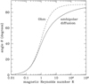 |
Fig. 2 Deflection angle 9 as a function of the magnetic Reynolds number RO (Eq. (6), dashed line) and Rad (Eq. (12), solid line). |
3.2 Numerical values
With the usual parametrization ρi = Cρ1/2, where C is a constant, the ambipolar diffusion resistivity Eq. (9) becomes
 (13)
(13)
The values of γ and C depend on the chemical composition of the medium. However, the combination γC is relatively well constrained, and can be conveniently expressed as γC = χ(8πG)1/2, where G is the gravitational constant and χ ≈ 1–3 (Pinto et al. 2008). This scaling reflects the relative importance of the ambipolar diffusion and free-fall time scales (Shu 1983), but in the present context in which the self-gravity of the filament is neglected, it is just a numerically convenient expression.
Inserting typical numerical values, with ρ = µmHn, where µ = 2.8 is the mean molecular weight,
 (14)
(14)

Thus, in principle, the direct evaluation of Rad from the curvature of the magnetic field lines allows to derive the magnetic field strength B0, provided the quantities a, u, and n are known.
Finally, the time to reach a steady state (ambipolar diffusion time) is
 (16)
(16)
and depends, if Rad is known, only on the filament’s size a and the flow velocity u.
4 Applications
In this section we apply the method described in Sects. 2 and 3 to two filaments in hub-filament systems, one in the Serpens South molecular cloud and one in the G327.3 high-mass star-forming region. Each filament has a mass of a few tens of solar masses, and is connected to a core/hub with a mass of a few hundreds of solar masses harboring a cluster of low-mass stars (in the Serpens South cloud) or a hot core (in G327.3). The physical parameters of the Serpens South and G327.3 filaments derived from observations, from the model with field-freezing (Sect. 2), and from the model with ambipolar diffusion (Sect. 3), are summarized in Table1.
4.1 Filaments in the Serpens South molecular cloud
The Serpens South molecular cloud is a nearby star-forming region that contains a young protostellar cluster embedded in a hub-filament system (Gutermuth et al. 2008). Kirk et al. (2013) found that these filaments show evidence of mass accretion flows, with rates similar to the star formation rate in the central cluster. Specifically, Kirk et al. (2013) measured a velocity gradient in the southern filament with a value of ∇uobs = 1.4 ± 0.2 km s−1 pc−1, over a projected length Lobs = 0.33 pc3. This measured velocity gradient corresponds to a flow with u = ∇uobs Lobs/ sin α, where 30° ≲ α ≲ 60° is the inclination of the filament with respect to the plane of the sky (Kirk et al. 2013). This gives a flow velocity  (here and in the following, the upper and lower values should be intended as extremes of a range, not an uncertainty).
Pillai et al. (2020) combine near- and far-infrared observations of polarized dust emission to map the magnetic field morphology in the Serpens South hub-filament system. They discovered a transition in the field orientation from approximately perpendicular to approximately parallel to the southern filament (referred to as FIL2) at visual extinctions above AV ≈ 20 mag up to AV ≈ 60 mag, that they interpreted as the consequence of the field being dragged by the gas flow. Specifically, the median deviation of polarization segments (magnetic field direction) from the parallel direction on either side of the filament, with diameter 2a = 0.1 pc, is 22° ± 3°, corresponding to an observed deflection angle θ = 78° ± 3°.
If the magnetic field pattern in the FIL2 region is interpreted in terms of Alfvén wings generated by the ballistic motion of perfectly conducting clumps in a magnetized medium, Eq. (1) implies a motion with Alfvén Mach number  . As mentioned in Sect. 2, highly super-Alfvénic motions are unlikely to be present in hub-filament systems, except, perhaps, near the central clump/hub. More importantly, as discussed in Sect. 2, a frozen-in magnetic field decelerates the fluid motion on a time scale of the order of the flow crossing time a/u times a factor δ or δ1/2, where δ is the density contrast between the filament and the environment. With the values of a and u estimated for the FIL2 region, the flow crossing time is
  . Although the factor δ is difficult to estimate, the deceleration time scale of the flow in the FIL2 region appears to be quite short, making the field-freezing model implausible.
On the other hand, in the framework of ambipolar diffusiondominated flows modeled in Sect. 3, the observed range of 9 corresponds to  (see Eq. (12) and Fig. 2), an acceptable value for dense gas (Myers & Khersonsky 1995). From Eq. (16), the time scale needed to reach an advection-diffusion steady state is
  Myr, which is compatible with the age of Serpens Main, the youngest cluster in the Serpens molecular cloud (~4 Myr, Zhou et al. 2022)4. In this case, an estimate of the magnetic field strength in the FIL2 region can be obtained from Eq. (15), if the filament’s average density n is known. This quantity can be estimated as follows. The range of visual extinction 20–60 mag corresponds to an observed H2 column density Nobs = (3.8 ± 1.9) × 1022 cm−2. Assuming a cylindrical filament with diameter 2a, the density n = 2Nobs cos α/(πa) is
  . Eq. (15) with χ = 3 then gives a magnetic field strength
  . With the central values of Nobs, α and B0, the non-dimensional mass-to-flux ratio λ ≈ 7.6 (Nobs cos α/1021 cm−2)(B0/µG)−1 (Crutcher 2004) is λ ≈ 3.0, albeit with large uncertainties. Kusune et al. (2019) apply the Davis-Chandrasekhar-Fermi method (see Sect. 4.2) to model near-infrared polarization data in the same region analyzed here, finding Bpos = 36 µG and λ = 3.6, compatible with our results.
Parameters for the Serpens South and G327.3 filament: field-freezing vs. magnetic diffusion.
4.2 Filaments in the high-mass star-forming region G327.3
The high-mass star-forming region G327.3 is a massive star-forming region characterized by filamentary structures connected to a central massive hot core. Beuther et al. (2020) conduct sub-mm continuum and polarization observations of G327.3 discovering filamentary structures characterized with U-shaped magnetic field morphologies pointing toward the central core (see their Fig. 1). One of these structures, the filament NE1-NE2, has a width of 2.5″ (equivalent to a full size of 2a = 7750 au at the distance of 3.1 kpc), a range of H2 column densities Nobs = (4.3 ± 2.7) × 1023 cm−2, and a small inclination α ≈ 9° with respect to the plane of the sky. As in the case of the Serpens South filament, assuming a cylindrical geometry, the mean density is in the range n = (4.6 ± 3.0) × 106 cm−3.
The filamentary structures in the G327.3 system were interpreted by Beuther et al. (2020) as indicative of channel flows feeding star formation in the central hot core. To test this hypothesis with the diffusive flow model developed in Sect. 3, we used the DustPol module of the ARTIST package (Padovani et al. 2012) to produce synthetic polarization maps of the filament NE1-NE2. DustPol computes the Stokes parameters I, Q and U from the expressions given in Padovani et al. (2012), originally derived by Lee & Draine (1985). A uniform dust temperature was assumed. The output maps are then processed with the simobserve and simanalyze tasks of the CASA programme5, adopting the same antenna configuration as in the observing runs. A best-fit of the polarization data is obtained for a magnetic Reynolds number Rad = 16. Figure 3 shows the comparison between the observed polarization segments and those from the best fit model. Unfortunately no information is available about the existence of a longitudinal accretion flow in the filament: the almost face-on orientation of this hub-filament system, favorable to the modeling of dust polarization data, makes it difficult to measure a velocity gradient. From the first moment map of 13CH3CN(124-114) of Beuther et al. (2020), an upper limit on the line-of-sight component of the flow velocity ulos < 0.21 km s−1 can be derived. For an inclination α ≈ 9°, this implies u < ulos/sin α = 1.3 km s−1. Assuming u = 1 km s−1, Eq. (15) with χ = 3 gives  mG. With the central values of Nobs, α and B0, the non-dimensional mass-to-flux ratio is λ ≈ 2.2. If, instead, u = 0.5 km s−1, the magnetic field strength would be reduced by a factor of
  , the ambipolar diffusion time would be 2 times larger, and the mass-to-flux ratio a factor of
  larger (Table 1). In either case, the magnetic field strength is higher than in the case of the Serpens South cloud (and therefore the bending of field lines less strong), consistently with the higher density and mass of the G327.3 star-forming region. The time needed to reach an advection-diffusion balance, from Eq. (16), is tad = 2.8−5.6 × 10⁵ yr. Although the evolutionary age of G327.3 is not known, this timescale is not incompatible with the dynamical characteristics of the central hot core (Leurini et al. 2017).
As a further check, one can estimate the strength of the component of the magnetic field in the plane of the sky Bpos in the NE1-NE2 filament. This can be done by applying the Davis-Chandrasekhar-Fermi formula (Davis 1951; Chandrasekhar & Fermi 1953),
 (17)
(17)
In Eq. (17), ξ is a correction factor typically set to 0.5 based on simulation of turbulent clouds (Ostriker et al. 2001), σlos is the line-of-sight velocity dispersion, and σψ is the standard deviation of polarization angle residuals. Figure 4 shows the distribution of polarization angle residuals Δψ = ψobs − ψmod for the best-fit model. By fitting a Gaussian to the distribution of residuals, we find a mean value of 〈Δψ〉 = −1.1° and a standard deviation σψ = 18°. Unfortunately, the 13CH3CN(124−114) data of Beuther et al. (2020) only have a spectral resolution of 2.7km s−1, and the line width σlos cannot be determined. For the purpose of demonstration we assume σlos = 1 km s−1, a reasonable value for high-mass star forming regions (Beltrán et al. 2019, 2024). With this value of σlos, along with the range of n given above, we obtain  , which is consistent with the estimates of B derived above from the analysis of the field curvature. The revised Davis-Chandrasekhar-Fermi formula proposed by Skalidis & Tassis (2021),
 (18)
(18)
gives a slightly smaller value of  . A magnetic field strength of similar magnitude has been estimated by Beltrán et al. (2019, 2024) in the outer regions of the high-mass star forming region G31.41+031.
As in the case of the Serpens South filament, an interpretation of the polarization pattern in terms of a frozen-in magnetic field distorted by the motions of clumps NE1 and NE2 toward the central hot core results in a high magnetic Alfvén Mach number, MA = 3.3. More importantly, the magnetic braking time of the motion of the clumps is within a factor δ or δ1/2 of the flow crossing time a/u = 1.8−3.6 × 10⁴ yr. Therefore, as in the case of the Serpens South filament, we conclude that the interpretation based on the diffusive model is more realistic.
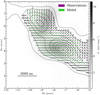 |
Fig. 3 Map of polarization segments (rotated by 90°) and polarized intensity P (greyscale) in the NE1-NE2 filament in the high-mass star-forming region G327.7: observations (purple), from Beuther et al. (2020); best-fit model (green). The black contours show the observed 1.3 mm dust emission intensity starting from 3σ in steps of 6σ. |
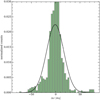 |
Fig. 4 Histogram of polarization angle residuals Δψ = ψobs − ψmod for our best-fit model in the region shown in Fig. 3 inside the 6σ contour of the 1.3 mm dust continuum map. The black curve is a Gaussian with mean 〈Δψ〉 = −1.1° and standard deviation σψ = 18°. |
5 Discussion
The deflection angle θ of magnetic field lines analyzed in Sects. 2 and 3 can be considered as a rough measure of the magnetic field curvature  , where
  (Boozer 2004). This geometrical parameter is connected to the physical characteristics of the field and the underlying flow (Yang et al. 2019). If the velocity field has a typical lifetime shorter than the crossing time scale a/u, the curvature of the field depends on the Alfvén Mach number of the flow MA, as discussed in Sect. 2. This is the case of turbulent velocity fields, where the time correlation extends no farther than a/u. The scaling of the magnetic field curvature with the Alfvén Mach number is in fact a characteristic of magnetohydrodynamical turbulence (Yuen & Lazarian 2020). In the opposite limit of a flow driven on a time scale longer than the diffusion time across the flow region, as in the cases studied here, the diffusive 2-D models of Sect. 3, Eq. (6) or Eq. (12) provide the relationship between k and RO or Rad, respectively.
Models of diffusive magnetic field transport have frequently been developed in the past to describe the radial flow in accretion disks adopting an axisymmetric thin-disk geometry. Wardle & Konigl (1990) proposed a relationship equivalent to Eq. (6) between the bending of field lines and the magnetic Reynolds number of the radial motion in their self-similar model of the Galactic center disk6; Lubow et al. (1994) numerically confirmed Eq. (6) for the accretion flow in a protostellar viscous disk. In both these models the disk half-width H is proportional to the disk radius ϖ, and the magnetic Reynolds number R = Hu/η is constant with ϖ: in the model of Wardle & Konigl (1990) u is constant and η ∝ ϖ; in the model of Lubow et al. (1994) u ∝ ϖ−1 and η is constant.
The dependence of the magnetic Reynolds number on the spatial scale is important, because it determines the degree of coupling of the field to the gas and the curvature of the magnetic field lines. In a spherical free-falling cloud with u ∝ r−1/2, the magnetic Reynolds number R = ru/η ∝ r1/2 increases with r (for η constant). Therefore fieldlines are aligned with the flow at large radii and straight and uniform close to the central protostar where the field decouples from the gas (Shu et al. 2006). Conversely, a gravity-driven free-fall flow with uniform resistivity in a filament with constant width has a magnetic Reynolds number R = au/η ∝ r−1/2 that decreases outward. At large distance from the center of gravitational attraction, the field is relatively unaffected by the flow (i.e., almost uniform), but becomes increasingly coupled to the fluid (i.e., more pinched) approaching the center of attraction (see Fig. 16 of Wang et al. 2020). A hint of increased curvature of the fieldlines can be seen in the bottom right corner of Fig. 3, where the filament in the G327.7 region merges with the central core. However, for simplicity, in this work we have considered flows with constant a, u and η.
A more serious simplification of our model is the neglect of self-gravity: Fig. 3 shows the presence in the G327.7 filament of two concentrations of dust emission intensity suggesting the onset of fragmentation, in agreement with the magnetically super-critical state of the filament found in Sect. 4.2. However, the magnetic field revealed by the dust polarization pattern seems to be unaffected by the gravitational attraction of the two concentrations.
Finally, it should be kept in mind that the problem of reconstructing the morphology of the magnetic field morphology from dust polarization maps is well-known for being degenerate (see, e.g., Reissl et al. 2018). Even for the simple geometry assumed in this study, projection effects impact the applicability of the model: a U-shaped magnetic field line may appear more or less curved than it actually is, depending on the viewing direction, or may not appear curved at all (Gómez et al. 2018); also, the derivation of the flow velocity along the filament from the observed velocity gradient depends on the inclination of the filament with respect to the plane of the sky, which is generally unknown. The discussion of Sect. 4 highlights the need to complement dust polarization observations with accurate kinematic and spectroscopic data, a task that requires, among other things, the selection of sources with known inclinations with respect to the plane of the sky. Another limitation of the applicability of the diffusive model of Sect. 3 is the slow convergence of θ to 90° for large values of the magnetic Reynolds number (see Fig. 2). This slow convergence implies a significant uncertainty in the value of the magnetic Reynolds number, even for a relatively well-constrained value of θ. However, comparing the method with specific cases can at least provide a consistency check on the amount of magnetic diffusivity required to maintain a steady-state filamentary accretion, as well as a rough estimate of the time scale needed to reach such a state.
6 Conclusions
We have elaborated the idea of Gómez et al. (2018), suggesting that that the curvature of magnetic field lines in filamentary molecular clouds, as inferred from polarization maps, could provide insights into the properties of accretion flows that feed star formation at the intersection of filaments (hubs). Given the clumpy appeareance of most filaments, at first sight it seems reasonable to consider that the frozen-in magnetic field, being dragged by moving inhomogeneities, could form bow wakes known as Alfvén wings. These wings would be characterized by an opening angle dependent on the Alfvén Mach number of the flow (see Sect. 2). However, the accumulation of the swept-up magnetic field in front of a highly conducting moving body leads to a deceleration of the flow within a time scale comparable to the flow crossing time, implying that filaments cannot be persistent structures. Furthermore, in the Alfvén wings scenario, the observed bending of the field would imply significantly large values of the Alfvén Mach number.
If, on the other hand, filaments in hub-filament systems have long lifetimes and transport a significant amount of mass to the central core, a steady-state accretion flow can be established on a time scale of the order of the flow crossing time a/u times the magnetic Reynolds number. In this steady state, the inward advection of magnetic field, driven by an external source, is balanced by magnetic field diffusion (see Sect. 3). Ambipolar diffusion can provide the necessary decoupling between the magnetic field and the flowing matter. The two examples analyzed in this study demonstrate that this scenario is consistent with the observed data, while an interpretation based on field-freezing appears less plausible. It must be stressed, however, that the interpretation of velocity gradients in terms of gas inflow along the filaments toward the hubs needs to be fully verified by observations.
Table 1 summarizes the physical characteristics of the two regions analyzed here according to the two interpretations. Our results support a general picture in which a star-forming core (the hub) keeps gaining mass by accretion along filaments over most of its lifetime, without the need to accumulate all of its mass during a pre-stellar core phase. Being magnetically supercritical, the filaments studied in this work are expected to disperse by fragmentation and collapse. In the FIL2 filament in the Serpens South cloud Friesen & Jarvis (2024) identify ~5 cores gravitationally bound, with a mass of a few solar masses each. However, unlike their isolated counterparts, hub-feeding filaments are strongly affected by protostellar feedback from the forming stellar cluster, which eventually leads to the dispersal of the network of filaments (Wang et al. 2010), and by the strong gravitational pull of the central core, as suggested by the evidence of gas acceleration in the proximity of the hub (Hacar et al. 2017; Zhou et al. 2023; Sen et al. 2024).
Further validation of the basic findings in this study can be obtained by generating synthetic dust polarization maps using models that incorporate more realistic filament geometry and flow properties. Since grid-based codes have a high intrinsic numerical viscosity vnum of the order of 1023 cm2 s−1 (McKee et al. 2020), albeit dependent on resolution, and have a numerical magnetic Prandtl number Pnum = vnum/ηnum ~ 1–2, as argued by Lesaffre & Balbus (2007), then the numerical resistivity of MHD simulations is quite large, of the order of the resistivity provided by ambipolar diffusion in the typical conditions of filaments. Therefore it is possible that current ideal MHD simulations of filament formation and evolution are in fact showing the effects of diffusion-dominated gas flows outlined in this work.
Acknowledgements
We thank the referee, whose comments and suggestions resulted in an improved final version of this paper. D.G. and M.P. acknowledge support from INAF large grant “The role of MAGnetic fields in MAssive star formation” (MAGMA).
References
- Arzoumanian, D., Furuya, R. S., Hasegawa, T., et al. 2021, A&A, 647, A78 [NASA ADS] [CrossRef] [EDP Sciences] [Google Scholar]
- Baumjohann, W., Blanc, M., Fedorov, A., & Glassmeier, K.-H. 2010, Space Sci. Rev., 152, 99 [NASA ADS] [CrossRef] [Google Scholar]
- Beltrán, M. T., Padovani, M., Girart, J. M., et al. 2019, A&A, 630, A54 [Google Scholar]
- Beltrán, M. T., Padovani, M., Galli, D., et al. 2024, A&A, 686, A281 [NASA ADS] [CrossRef] [EDP Sciences] [Google Scholar]
- Beuther, H., Soler, J. D., Linz, H., et al. 2020, ApJ, 904, 168 [NASA ADS] [CrossRef] [Google Scholar]
- Blandford, R. D., & Payne, D. G. 1982, MNRAS, 199, 883 [CrossRef] [Google Scholar]
- Boozer, A. H. 2004, Rev. Mod. Phys., 76, 1071 [Google Scholar]
- Chandrasekhar, S., & Fermi, E. 1953, ApJ, 118, 113 [Google Scholar]
- Chapman, N. L., Goldsmith, P. F., Pineda, J. L., et al. 2011, ApJ, 741, 21 [NASA ADS] [CrossRef] [Google Scholar]
- Chen, Z., Sefako, R., Yang, Y., et al. 2023, MNRAS, 525, 107 [CrossRef] [Google Scholar]
- Cox, N. L. J., Arzoumanian, D., André, P., et al. 2016, A&A, 590, A110 [NASA ADS] [CrossRef] [EDP Sciences] [Google Scholar]
- Crutcher, R. M. 2004, Ap&SS, 292, 225 [NASA ADS] [CrossRef] [Google Scholar]
- Dall’Olio, D., Vlemmings, W. H. T., Persson, M. V., et al. 2019, A&A, 626, A36 [NASA ADS] [CrossRef] [EDP Sciences] [Google Scholar]
- Davidson, P. A. 2001, An Introduction to Magnetohydrodynamics (Cambridge) [CrossRef] [Google Scholar]
- Davis, L. 1951, Phys. Rev., 81, 890 [Google Scholar]
- Drell, S. D., Foley, H. M., & Ruderman, M. A. 1965, J. Geophys. Res., 70, 3131 [Google Scholar]
- Dursi, L. J., & Pfrommer, C. 2008, ApJ, 677, 993 [NASA ADS] [CrossRef] [Google Scholar]
- Ebert, R., von Hoerner, S., & Temesváry, S. 1960, in Die Entstehung von Sternen durch Kondensation diffuser Materie (Springer), 184 [CrossRef] [Google Scholar]
- Faraday, M. 1832, Philos. Trans. Roy. Soc. London, 122, 163 [NASA ADS] [CrossRef] [Google Scholar]
- Fernández-López, M., Arce, H. G., Looney, L., et al. 2014, ApJ, 790, L19 [Google Scholar]
- Fiege, J. D., & Pudritz, R. E. 2000, MNRAS, 311, 85 [Google Scholar]
- Friesen, R. K., & Jarvis, E. 2024, ApJ, submitted [arXiv:2404.07259] [Google Scholar]
- Friesen, R. K., Medeiros, L., Schnee, S., et al. 2013, MNRAS, 436, 1513 [NASA ADS] [CrossRef] [Google Scholar]
- Gómez, G. C., Vázquez-Semadeni, E., & Zamora-Avilés, M. 2018, MNRAS, 480, 2939 [Google Scholar]
- Gutermuth, R. A., Bourke, T. L., Allen, L. E., et al. 2008, ApJ, 673, L151 [NASA ADS] [CrossRef] [Google Scholar]
- Gutiérrez-Vera, N., Grassi, T., Bovino, S., et al. 2023, A&A, 670, A38 [NASA ADS] [CrossRef] [EDP Sciences] [Google Scholar]
- Hacar, A., Alves, J., Tafalla, M., & Goicoechea, J. R. 2017, A&A, 602, L2 [NASA ADS] [CrossRef] [EDP Sciences] [Google Scholar]
- Hwang, J., Kim, J., Pattle, K., et al. 2022, ApJ, 941, 51 [NASA ADS] [CrossRef] [Google Scholar]
- Jones, T. W., Kang, H., & Tregillis, I. L. 1994, ApJ, 432, 194 [Google Scholar]
- Jones, T. W., Ryu, D., & Tregillis, I. L. 1996, ApJ, 473, 365 [NASA ADS] [CrossRef] [Google Scholar]
- Juárez, C., Girart, J. M., Zamora-Avilés, M., et al. 2017, ApJ, 844, 44 [Google Scholar]
- Kirk, H., Myers, P. C., Bourke, T. L., et al. 2013, ApJ, 766, 115 [Google Scholar]
- Kivelson, M. G., Bagenal, F., Kurth, W. S., et al. 2007, in Jupiter (Cambridge), 513 [Google Scholar]
- Koch, P. M., Tang, Y.-W., Ho, P. T. P., et al. 2022, ApJ, 940, 89 [NASA ADS] [CrossRef] [Google Scholar]
- Kusune, T., Nakamura, F., Sugitani, K., et al. 2019, PASJ, 71, S5 [NASA ADS] [CrossRef] [Google Scholar]
- Lee, H. M., & Draine, B. T. 1985, ApJ, 290, 211 [Google Scholar]
- Lesaffre, P., & Balbus, S. A. 2007, MNRAS, 381, 319 [NASA ADS] [CrossRef] [Google Scholar]
- Leurini, S., Herpin, F., van der Tak, F., et al. 2017, A&A, 602, A70 [NASA ADS] [CrossRef] [EDP Sciences] [Google Scholar]
- Li, G.-X., Wyrowski, F., & Menten, K. 2017, A&A, 598, A96 [NASA ADS] [CrossRef] [EDP Sciences] [Google Scholar]
- Linker, J. A., Kivelson, M. G., & Walker, R. J. 1991, J. Geophys. Res., 96, 21037 [NASA ADS] [CrossRef] [Google Scholar]
- Liu, T., Li, P. S., Juvela, M., et al. 2018, ApJ, 859, 151 [NASA ADS] [CrossRef] [Google Scholar]
- Lubow, S. H., Papaloizou, J. C. B., & Pringle, J. E. 1994, MNRAS, 267, 235 [NASA ADS] [Google Scholar]
- Lundquist, S. 1952, Arkiv. Fisik, 5, 297 [Google Scholar]
- Lyutikov, M. 2006, MNRAS, 373, 73 [CrossRef] [Google Scholar]
- McKee, C. F., Stacy, A., & Li, P. S. 2020, MNRAS, 496, 5528 [NASA ADS] [CrossRef] [Google Scholar]
- Mookerjea, B., Veena, V. S., Güsten, R., Wyrowski, F., & Lasrado, A. 2023, MNRAS, 520, 2517 [NASA ADS] [CrossRef] [Google Scholar]
- Mouschovias, T. C. 1977, ApJ, 211, 147 [NASA ADS] [CrossRef] [Google Scholar]
- Myers, P. C. 2009, ApJ, 700, 1609 [Google Scholar]
- Myers, P. C., & Khersonsky, V. K. 1995, ApJ, 442, 186 [NASA ADS] [CrossRef] [Google Scholar]
- Nagasawa, M. 1987, Progr. Theor. Phys., 77, 635 [NASA ADS] [CrossRef] [Google Scholar]
- Neubauer, F. M. 1980, J. Geophys. Res., 85, 1171 [Google Scholar]
- Ortiz-León, G. N., Loinard, L., Dzib, S. A., et al. 2018, ApJ, 869, L33 [Google Scholar]
- Ostriker, E. C., Stone, J. M., & Gammie, C. F. 2001, ApJ, 546, 980 [Google Scholar]
- Padovani, M., Brinch, C., Girart, J. M., et al. 2012, A&A, 543, A16 [NASA ADS] [CrossRef] [EDP Sciences] [Google Scholar]
- Pan, S., Liu, H.-L., & Qin, S.-L. 2024, ApJ, 960, 76 [NASA ADS] [CrossRef] [Google Scholar]
- Parker, E. N. 1963, ApJ, 138, 552 [NASA ADS] [CrossRef] [Google Scholar]
- Pattle, K., Fissel, L., Tahani, M., Liu, T., & Ntormousi, E. 2023, in Protostars and Planets VII (Astronomical Society of the Pacific), 193 [Google Scholar]
- Pillai, T. G. S., Clemens, D. P., Reissl, S., et al. 2020, Nat. Astron., 4, 1195 [Google Scholar]
- Pinto, C., Galli, D., & Bacciotti, F. 2008, A&A, 484, 1 [NASA ADS] [CrossRef] [EDP Sciences] [Google Scholar]
- Planck Collaboration Int. XXXV. 2016, A&A, 586, A138 [NASA ADS] [CrossRef] [EDP Sciences] [Google Scholar]
- Reissl, S., Stutz, A. M., Brauer, R., et al. 2018, MNRAS, 481, 2507 [NASA ADS] [CrossRef] [Google Scholar]
- Roberts, P. H. 1967, An Introduction to Magnetohydrodynamics (Longmans) [Google Scholar]
- Sanhueza, P., Girart, J. M., Padovani, M., et al. 2021, ApJ, 915, L10 [NASA ADS] [CrossRef] [Google Scholar]
- Schwörer, A., Sánchez-Monge, Á., Schilke, P., et al. 2019, A&A, 628, A6 [NASA ADS] [CrossRef] [EDP Sciences] [Google Scholar]
- Sen, S., Mookerjea, B., Güsten, R., Wyrowski, F., & Ishwara Chandra, C. H. 2024, ApJ, 967, 151 [Google Scholar]
- Shu, F. H. 1983, ApJ, 273, 202 [NASA ADS] [CrossRef] [Google Scholar]
- Shu, F. H., Galli, D., Lizano, S., & Cai, M. 2006, ApJ, 647, 382 [NASA ADS] [CrossRef] [Google Scholar]
- Skalidis, R., & Tassis, K. 2021, A&A, 647, A186 [NASA ADS] [CrossRef] [EDP Sciences] [Google Scholar]
- Toci, C., & Galli, D. 2015a, MNRAS, 446, 2110 [NASA ADS] [CrossRef] [Google Scholar]
- Toci, C., & Galli, D. 2015b, MNRAS, 446, 2118 [NASA ADS] [CrossRef] [Google Scholar]
- Tomisaka, K. 2014, ApJ, 785, 24 [Google Scholar]
- Treviño-Morales, S. P., Fuente, A., Sánchez-Monge, Á., et al. 2019, A&A, 629, A81 [NASA ADS] [CrossRef] [EDP Sciences] [Google Scholar]
- Wang, P., Li, Z.-Y., Abel, T., & Nakamura, F. 2010, ApJ, 709, 27 [NASA ADS] [CrossRef] [Google Scholar]
- Wang, J.-W., Koch, P. M., Galván-Madrid, R., et al. 2020, ApJ, 905, 158 [Google Scholar]
- Wang, J.-W., Koch, P. M., Tang, Y.-W., et al. 2022, ApJ, 931, 115 [NASA ADS] [CrossRef] [Google Scholar]
- Wardle, M., & Konigl, A. 1990, ApJ, 362, 120 [NASA ADS] [CrossRef] [Google Scholar]
- Yang, Y., Wan, M., Matthaeus, W. H., et al. 2019, Phys. Plasmas, 26, 072306 [NASA ADS] [CrossRef] [Google Scholar]
- Yuan, J., Li, J.-Z., Wu, Y., et al. 2018, ApJ, 852, 12 [Google Scholar]
- Yuen, K. H., & Lazarian, A. 2020, ApJ, 898, 66 [NASA ADS] [CrossRef] [Google Scholar]
- Zamora-Avilés, M., Ballesteros-Paredes, J., & Hartmann, L. W. 2017, MNRAS, 472, 647 [Google Scholar]
- Zhou, X., Herczeg, G. J., Liu, Y., Fang, M., & Kuhn, M. 2022, ApJ, 933, 77 [NASA ADS] [CrossRef] [Google Scholar]
- Zhou, J. W., Wyrowski, F., Neupane, S., et al. 2023, A&A, 676, A69 [NASA ADS] [CrossRef] [EDP Sciences] [Google Scholar]
Faraday unsuccessfully attempted to measure the electric current induced by the Thames River flowing in the Earth’s magnetic field (Faraday 1832).
The right-hand side of Eq. (3) should be equal to the gradient in the y-direction of a function ϕ. However, since there cannot be a y-dependence in this 2-D problem, ∇ϕ is at most a constant representing a uniform electric field in the y-direction. In the absence of such an external electric field, the induction equation takes the form of Eq. (3).
Kirk et al. (2013) assumed a distance to the Serpens cloud of 260 pc, smaller than the value currently adopted of 436 pc (Ortiz-León et al. 2018). However the correction for distance cancels out in the product of ∇uobsLobs.
Wardle & Konigl (1990) found that a value of the magnetic Reynolds number (referred to as βδ) equal to 3.4 can reproduce a set of polarization measurements in the Galactic center region.
All Tables
Parameters for the Serpens South and G327.3 filament: field-freezing vs. magnetic diffusion.
All Figures
|
Fig. 1 Steady-state magnetic field lines for a flow with uniform resistivity and uniform velocity u (arrows) in a transverse magnetic field. for different values of the magnetic Reynolds number: R = 0.5, 1, 2, 4, 10 and 50. Solid lines: with ambipolar diffusion (R = Rad); dashed lines: with Ohmic resistivity (R = RO). The flow is limited to the region −a < z < a. The deflection angle θ is also shown. |
| In the text | |
|
Fig. 2 Deflection angle 9 as a function of the magnetic Reynolds number RO (Eq. (6), dashed line) and Rad (Eq. (12), solid line). |
| In the text | |
|
Fig. 3 Map of polarization segments (rotated by 90°) and polarized intensity P (greyscale) in the NE1-NE2 filament in the high-mass star-forming region G327.7: observations (purple), from Beuther et al. (2020); best-fit model (green). The black contours show the observed 1.3 mm dust emission intensity starting from 3σ in steps of 6σ. |
| In the text | |
|
Fig. 4 Histogram of polarization angle residuals Δψ = ψobs − ψmod for our best-fit model in the region shown in Fig. 3 inside the 6σ contour of the 1.3 mm dust continuum map. The black curve is a Gaussian with mean 〈Δψ〉 = −1.1° and standard deviation σψ = 18°. |
| In the text | |
Current usage metrics show cumulative count of Article Views (full-text article views including HTML views, PDF and ePub downloads, according to the available data) and Abstracts Views on Vision4Press platform.
Data correspond to usage on the plateform after 2015. The current usage metrics is available 48-96 hours after online publication and is updated daily on week days.
Initial download of the metrics may take a while.