| Issue |
A&A
Volume 689, September 2024
|
|
|---|---|---|
| Article Number | A282 | |
| Number of page(s) | 10 | |
| Section | Galactic structure, stellar clusters and populations | |
| DOI | https://doi.org/10.1051/0004-6361/202449791 | |
| Published online | 19 September 2024 | |
Cluster membership analysis with supervised learning and N-body simulations
1
Department of Physics, Xi’an Jiaotong-Liverpool University,
111 Ren’ai Road, Dushu Lake Science and Education Innovation District, Suzhou
215123,
Jiangsu Province,
PR
China
2
Energetic Cosmos Laboratory, Nazarbayev University,
53 Kabanbay Batyr Ave.,
010000
Astana,
Kazakhstan
3
Heriot-Watt University Aktobe Campus,
263 Zhubanov Brothers Str,
030000
Aktobe,
Kazakhstan
4
Heriot-Watt International Faculty, K. Zhubanov Aktobe Regional University,
263 Zhubanov Brothers Str,
030000
Aktobe,
Kazakhstan
5
Fesenkov Astrophysical Institute,
23 Observatory Str.,
050020
Almaty,
Kazakhstan
6
Faculty of Physics and Technology, Al-Farabi Kazakh National University,
71 Al-Farabi Ave,
050020
Almaty,
Kazakhstan
7
Department of Physics, School of Sciences and Humanities, Nazarbayev University,
53 Kabanbay Batyr Ave.,
010000
Astana,
Kazakhstan
8
Shanghai Key Laboratory for Astrophysics, Shanghai Normal University,
100 Guilin Road,
Shanghai
200234,
PR
China
9
Nicolaus Copernicus Astronomical Centre Polish Academy of Sciences,
ul. Bartycka 18,
00-716
Warsaw,
Poland
10
Konkoly Observatory, HUN-REN Research Centre for Astronomy and Earth Sciences,
Konkoly Thege Miklós út 15–17,
1121
Budapest,
Hungary
11
Main Astronomical Observatory, National Academy of Sciences of Ukraine,
27 Akademika Zabolotnoho St.,
03143
Kyiv,
Ukraine
Received:
29
February
2024
Accepted:
27
July
2024
Context. Membership analysis is an important tool for studying star clusters. There are various approaches to membership determination, including supervised and unsupervised machine-learning (ML) methods.
Aims. We perform membership analysis using the supervised ML approach.
Methods. We trained and tested our ML models on two sets of star cluster data: snapshots from N-body simulations, and 21 different clusters from the Gaia Data Release 3 data.
Results. We explored five different ML models: random forest (RF), decision trees, support vector machines, feed-forward neural networks, and K-nearest neighbors. We find that all models produce similar results, and the accuracy of RF is slightly better. We find that a balance of classes in the datasets is optional for a successful learning. The classification accuracy strongly depends on the astrometric parameters. The addition of photometric parameters does not improve the performance. We find no strong correlation between the classification accuracy and the cluster age, mass, and half-mass radius. At the same time, models trained on clusters with a larger number of members generally produce better results.
Key words: methods: data analysis / methods: numerical / Galaxy: kinematics and dynamics / open clusters and associations: general / solar neighborhood
© The Authors 2024
 Open Access article, published by EDP Sciences, under the terms of the Creative Commons Attribution License (https://creativecommons.org/licenses/by/4.0), which permits unrestricted use, distribution, and reproduction in any medium, provided the original work is properly cited.
This article is published in open access under the Subscribe to Open model. Subscribe to A&A to support open access publication.
1 Introduction
The research of open clusters (OC) is essential in many areas of astronomy, including the formation and evolution of stars, Galactic dynamics, and star formation history (Lada & Lada 2003; de la Fuente Marcos & de la Fuente Marcos 2004; Krumholz et al. 2019). The reason is that the stars in a cluster tend to have the same age and kinematics (Portegies Zwart et al. 2010; Renaud 2018; Krumholz et al. 2019). To better estimate the fundamental parameters of star clusters such as age, mass, size, and metallicity, it is crucial to separate stars that are members from those that are in the field of the Galaxy (Kharchenko et al. 2005, 2012). This process is usually referred to as membership analysis.
Identifying member stars within OCs presents a significant challenge due to their location within the Galactic disk (Ascenso et al. 2009; Kharchenko et al. 2012). The subtle over-density generated by these clusters often becomes obscured by field stars (Bland-Hawthorn & Gerhard 2016). Historically, membership analysis relied heavily on manual methods (e.g. Stock 1956; Ruprecht et al. 1981; Phelps & Janes 1994; Chen et al. 2003; Kharchenko et al. 2005, 2012; Dias et al. 2014; Conrad et al. 2017; Röser et al. 2019; Meingast & Alves 2019; Lodieu et al. 2019). However, recent advancements in machine-learning (ML) and large datasets provided by Gaia Data Releases (Gaia Collaboration 2016a,b, 2018, 2021, 2023) have revolutionized this process (Olivares et al. 2023). Generally, supervised and unsupervised ML methods can be used (Sindhu Meena & Suriya 2020). While the supervised approach is based on training on labeled data, the unsupervised method does not rely on labeled data (Sindhu Meena & Suriya 2020). Numerous studies now leverage unsupervised learning techniques to automate and enhance the determination of cluster membership (Gao 2014; Cantat-Gaudin et al. 2018; Gao 2018b; Tang et al. 2019; Liu & Pang 2019; Castro-Ginard et al. 2020; Agarwal et al. 2021; Noormohammadi et al. 2023; Hunt & Reffert 2023, and more).
There are several types of unsupervised learning methods (Bishop 2006), including clustering, self-organized map algorithms, and probabilistic models (Bação et al. 2005). Among the clustering methods, the density-based algorithms have gained wide use (Gao 2014; Tucio et al. 2023; Ghosh et al. 2022). There are two versions of this method: a density-based spatial clustering of applications with noise (DBSCAN, Ester et al. 1996), and a hierarchical density-based spatial clustering of applications with noise (HDBSCAN, Campello et al. 2013). DBSCAN works by assigning (i.e., using hyperparameters) the radius and the minimum number of stars (Hunt & Reffert 2021). When the numbers of actual stars exceed these values, this region is classified as a cluster (Gao 2014). HDBSCAN works similarly but extends DBSCAN by constructing a cluster hierarchy based on minimum spanning trees (Hunt & Reffert 2021). This allows the handling of clusters of varying shapes and densities (Campello et al. 2013). Gao (2014) used DBSCAN on the 3D kinematic features of the NGC 188 cluster and identified 1504 member star candidates. Tucio et al. (2023) and Ghosh et al. (2022) used HDBSCAN to separate the member stars of NGC 2682 and NGC 7789 from field stars. The code UPMASK combines principle component analysis and clustering algorithms such as the k-means clustering implemented in the R language (Krone-Martins & Moitinho 2015). pyUPMASK is a Python implementation of the same method (Pera et al. 2021). StarGO (Yuan et al. 2018) is an unsupervised self-organized map algorithm that was initially built to find halo stars in the Galaxy. Tang et al. (2019) used it for dimensionality reduction and membership determination by using 5D kinematic data of stars. Later, this technique was used to find new OCs in the solar neighborhood (Liu & Pang 2019; Pang et al. 2020, 2022). Additionally, a probabilistic model such as the Gaussian mixture model (GMM) was used by Jaehnig et al. (2021), who applied it to 426 OCs.
Several attempts have also been made to use supervised learning in a membership analysis. A combination of unsupervised learning with supervised model methods was employed, such as random forest (RF) with GMM (Gao 2018a, a,b; Mahmudunnobe et al. 2021; Jadhav et al. 2021; Das et al. 2023; Guido et al. 2023) and K-nearest neighbors (KNN) with GMM (Agarwal et al. 2021; Deb et al. 2022). As for the supervised learning-only approach, van Groeningen et al. (2023) used deep sets neural networks on 167 OCs from the Gaia DR2 and eDR3 data based on the catalog of Cantat-Gaudin et al. (2020).
However, the membership analyses performed using different methods in previous studies show only a limited agreement with each other. For example, Bouma et al. (2021) reported that for OC NGC 2516, only 25% of the labels by Kounkel & Covey (2019), 41% of the labels by Meingast et al. (2021), and 68% of the labels by Cantat-Gaudin et al. (2018) overlap with each other.
In this work, we perform a membership analysis using supervised learning on data from simulations and observations for training and testing. For the former, we use the N-body simulations from Shukirgaliyev et al. (2021). The advantage of using simulation data is that we can determine the memberships of stars based on the physical conditions in the simulation. We use the Gaia DR3 data as the observational data and label the cluster members based on the findings of Liu & Pang (2019) and Pang et al. (2022).
This paper is organized as follows. Section 2 describes the method. Section 3 presents our results, and Sec. 4 provides our conclusions.
Sets of feature combinations.
2 Method
2.1 Data
We trained our ML models using data from N-body simulations and Gaia DR3 observations. When we used the simulation data, we considered eight observable parameters to describe the stars. These are the five astrometric parameters right ascension α, declination δ, two proper motions along these directions μα and μδ, the parallax π, and two photometric parameters: the apparent magnitude mG and the color index Gbp − Grp in the Gaia bands (Maíz Apellániz & Weiler 2018), and the radial velocity υr. To study the impact of these parameters, we explored different combinations of these parameters in our training and testing. For our default combination, which we call combination 1, we used a five-parameter family (α, δ, μα, μδ, and π). For parameter combination 2, we used α, δ, m, and Gbp − Grp. For combinations 3, 4, and 5, we used α, δ, μα, μδ, m, and Gbp − Grp, α, δ, μα, μδ, π, and υr, and α, δ, μα, μδ, π, m, and Gbp − Grp. Not all of these data combinations are available in the Gaia catalog. For this reason, when we tested and trained using the Gaia data, we only used the default combination (combination 1; see Table 1 for a summary).
2.1.1 N-body simulations
Our study is partially based on applications of supervised learning on N-body simulation data that cover the dynamic evolution from the gas expulsion to complete dissolution (Shukirgaliyev et al. 2017, 2021). The initial conditions are based on the Parmentier & Pfalzner (2013) model. We use the N-body simulation models of Shukirgaliyev et al. (2021) with Plummer density profile at the time of instantaneous gas expulsion. These are clusters of 104 stars that formed with three different global star formation efficiencies (SFEs) of 17%, 20%, and 25%. Shukirgaliyev et al. (2021) performed nine simulations per model with different randomization. We only use two randomizations of the position and mass labeled 11 and 22 by Shukirgaliyev et al. (2021). We did not use model clusters with the lowest SFE of 15% because they dissolve soon: Their star count in the aftermath of gas expulsion is low.
N-body simulations use Cartesian coordinates with an origin at the Galactic center (Shukirgaliyev et al. 2019). We then place the cluster at a distance of 150 pc from the Sun, as shown by Kalambay et al. (2022). We transfer the data to equatorial (International Celestial Reference System, ICRS) coordinates using the Astropy package (Astropy Collaboration 2013) to derive the five astrometric parameters α, δ, μα, μδ, and π. Using effective temperature, mass, metallicity, and luminosity of each star available in N-body simulations snapshots, we calculate the absolute magnitude corresponding to the Gaia DR2 (G, GBP, GRP, Maíz Apellániz & Weiler 2018) bands using the method described in Chen et al. (2019). Finally, with the knowledge of the parallaxes of all stars and their G, we calculate their apparent magnitudes (mg) using
![$\[m_G=G-5(\log \pi+1).\]$](/articles/aa/full_html/2024/09/aa49791-24/aa49791-24-eq1.png) (1)
(1)
We excluded dim stars with mG < 21 mag in the Gaia DR2 catalog from our analysis (Gaia Collaboration 2018).
To make our simulation data resemble actual astronomical observations, we generated field stars of the Galactic plane with the code Galaxia to produce a synthetic galaxy model (Sharma et al. 2011). We used the modified version by Rybizki (2019) to fit Gaia DR2. We then placed our cluster inside these stars. We labeled stars within the Jacobi radii (Just et al. 2009) as member stars, and those outside this radius were labeled as non-members. These nonmembers were member stars in earlier N-body simulation snapshots. The field stars obtained from Galaxia were also labeled nonmembers, but some may occur within the Jacobi radius of the cluster.
We considered a circular field of view around the cluster center that covered about 600 square degrees. This region included types of stars of the simulated cluster that are gravitationally bound and those that are unbound. We removed the tidal tail stars that are located outside this region. Nevertheless, some of the tail stars may appear in front of or behind the cluster by being projected onto the celestial sphere. Before applying ML, we moved the origin of our equatorial coordinate system to the cluster center. We determined the cluster center using the observational coordinates and proper motions using an iterative search of the density center. In this algorithm, the average coordinates (α and δ in our case) of all stars in our set were determined, and we shifted the coordinate origin to this location. Then, we repeated this process, considering stars within 80% of the maximum radius in the previous set until we reached the minimum threshold of 150 stars.
2.1.2 Gaia data
In addition to using data from N-body simulations, we also performed training and testing on clusters from the Gaia DR3 data (Gaia Collaboration 2023). From now on, we refer to Gaia DR3 as Gaia data. We trained three supervised ML models on Blanco 1, the Pleiades, and NGC 2516. We selected 21 clusters for testing: Blanco 1, Collinder 69, Huluwa 3, IC 4756, LP 2373 gp2, LP 2373 gp4, LP 2383, LP 2442, Mamajek 4, NGC 1980, NGC 2422, NGC 2451B, NGC 2516, NGC 3532, NGC 6405, NGC 6475, NGC 6633, the Pleiades, Praesepe, Stephenson 1, and UBC 31. We selected these clusters from the Pang et al. (2022) catalog. These clusters are classified by five morphological categories: filaments, fractals, halo, tidal tail, and unspecified (i.e., without clear morphological features outside one tidal radius). The 21 clusters that we selected contain clusters that belong to each of these categories (four filamentary clusters, four fractal clusters, three halo clusters, five tidal tail clusters, and five unspecified clusters). The data were retrieved from Astropy queries with a full inclusion of the field stars. The membership labeling data were taken from Pang et al. (2022). Since the member stars from Pang et al. (2022) are incomplete for mG < 21, we again excluded the dim stars with mG < 21 in the Gaia DR3 data from our analysis. This magnitude cut removed stars below 0.3 solar mass (Pang et al. 2024), but it does not affect our scientific motivation in this work.
2.2 Machine-learning
We tested five ML algorithms: KNN (Cover & Hart 1967), decision trees (DT, Breiman et al. 1984), RF (Breiman 2001), feed-forward neural network (FFNN, Bebis & Georgiopoulos 1994), and support vector machines (SVM, Cortes & Vapnik 1995).
The KNN is a simple, effective, and widely used ML model. It compares the distances of the KNN to a given sample for making predictions (Peterson 2009). The algorithm performance depends on K. Previously, the algorithm was used on the Gaia data in combination with the GMMs for membership identification (Agarwal et al. 2021). We used K = 5. The distance between neighbors is measured in terms of Minkowski distance. The probability of a cluster membership was calculated based on the distance weight function.
The supervised ML algorithm DT recursively splits the data based on features to create a tree-like structure (Fürnkranz 2010). We used a DT classifier from Scikit-learn (Pedregosa et al. 2011) with default parameters. To the best of our knowledge, this model has not yet been used in studies of OCs.
The ensemble learning ML algorithm RF uses multiple decision-tree predictors for classification and regression problems (Breiman 2001). This method was used in several studies that worked with Gaia data (Gao 2018a,b, 2019a; Mahmudunnobe et al. 2021; Das et al. 2023). We configured the model with 100 trees, a gini tree-split criterion, and did not specify the depth of the trees. We used an RF classifier from the Scikit-Learn library (Pedregosa et al. 2011).
The FFNN is the supervised ML model and is considered part of deep learning because the model depth depends on the number of layers (Bebis & Georgiopoulos 1994). The selection of an appropriate hyperparameters such as activation functions, optimization functions, learning rate, criterion, batch size, number of epochs, and number of layers is crucial for successful learning. We used five-layer neural networks with a batch size of 400 with activation functions such as LeakyReLU, Sigmoid, and GeLU and trained on 20 epochs with an Adam optimizer and the cross-entropy loss criterion. We used the PyTorch library (Paszke et al. 2019) to implement FFNN.
The SVM is a supervised ML algorithm that finds the optimal hyperplane that best separates different classes in the input feature space (Cortes & Vapnik 1995). To our knowledge, it was not used in previous studies on OC membership. We configured SVM with default hyperparameters from the Scikit-learn library (Pedregosa et al. 2011).
For the evaluation criteria, we used the confusion matrix, which is a matrix that shows the number of true positives (TP), true negatives (TN), false positives (FP), and false negatives (FN) of binary classification, as shown in Table 2. The diagonal part of the matrix is the correctly classified samples that are TN and TP (Kohl 2012). We measured the accuracy in terms of the F1 score accuracy (Goutte & Gaussier 2005),
![$\[F_1=\frac{2 \times \text { precision } \times \text { recall }}{\text { precision }+ \text { recall }},\]$](/articles/aa/full_html/2024/09/aa49791-24/aa49791-24-eq2.png) (2)
(2)
![$\[\text { precision }=\frac{\mathrm{TP}}{\mathrm{TP}+\mathrm{FP}}, \quad \text { recall }=\frac{\mathrm{TP}}{\mathrm{TP}+\mathrm{FN}}.\]$](/articles/aa/full_html/2024/09/aa49791-24/aa49791-24-eq3.png)
We trained our ML models on data from snapshots of N-body simulations and the Gaia DR3 data. The performance was not improved when a few snapshots were combined. For the N-body simulation data, we considered snapshots with different SFEs in different time frames. For the default case, we used the snapshot at the end of the violent relaxation at 20 Myr of the model cluster with an SFE of 17%. We also considered snapshots at 100 Myr and 500 Myr, as discussed below.
For the testing, we used snapshots from simulations with different SFEs. These simulations included a randomization for positions and masses that were different from those of the training set. When we added field stars, we used snapshots at 100 Myr and 1 Gyr. An example testing set of model clusters with an SFE of 17% in a 20 Myr snapshot combined with field stars is shown in Fig. 1.
Confusion matrix representing the performance of the prediction compared to the actual value.
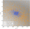 |
Fig. 1 Stars from N-body simulation with an SFE of 17% in a 20 Myr snapshot with generated field stars projected onto the sky. The blue, orange, and gray points show the member, nonmember, and Galactic field stars. |
3 Results
All the results shown below were obtained using the RF method. The dependence on the ML methods is described in Appendix A.
3.1 Test on N-body simulation data
We first applied ML to N-body simulation data. For our first training, we selected a snapshot at 20 Myr for a simulation with an SFE of 17%. This snapshot corresponds to the system equilibrium phase after violent relaxation.
The upper panel of Fig. 2 shows the F1 score as a function of time for different testing sets. We first discuss the case with an SFE of 17%, shown in black. In the initial phase (t ≲ 200 Myr), the accuracy is ≈95%. It starts to decrease with time at t ≈ 200 Myr and reaches ≈77.5% at t ≈ 1 Gyr. The drop in accuracy is correlated with the size and mass of the cluster, which shrink over time, as shown in the bottom panel of Fig. 2. Most of the mistakes in later snapshots are due to an increase in FP classifications.
The classification accuracy for simulations with a higher SFE is qualitatively similar to an SFE of 17%, but has some modest quantitative differences. The red and blue lines show the F1 score accuracy as a function of time for tests with an SFE of 20% and SFE of 25%. At t ≲ 200 Myr, the accuracies are ≈98.0% and ≈97.5 for an SFE of 20% and an SFE of 25%, respectively. The F1 scores start to decrease with time at t ≈ 1 Gyr and t ≈ 2 Gyr for an SFE of 20% and an SFE of 25%, respectively. The lowest value for an SFE of 20% is F1 ≈ 68% at t ≈ 1.557 Gyr, and for an SFE of 25%, it is F1 ≈ 83% at t ≈ 3 Gyr.
Next, we explored the dependence of training sets on the time and SFE of N-body simulation snapshots. We trained nine models on snapshots of three model clusters with different SFEs (17, 20, and 25%) at three times (20, 100, and 500 Myr). We tested each model on 1096 snapshots with different times and SFEs representing the full snapshots of all N-body simulations we used. Figure 3 shows the F1 score as box plots for different values of t and SFE. The center of the box corresponds to the median F1 score value, while the upper and lower boundaries correspond to 25% quantiles. The error bars represent the maximum and minimum values. Overall, the differences in accuracies between different training sets are minor. The average accuracy varies between F1 ≈ 95% to F1 ≈ 97%. The upper quantiles are between ≈97% and ≈ 99%, and the maximum values are ≈99%. The lower quantiles are between 89.0% and ≈93.5%, and the minimum values are between 63% and 73%. We also trained our models on a combination of up to ten snapshots, but the resulting accuracy was not higher than that for models trained with only one snapshot.
Next, we explored the impact of the stellar parameters on the classification accuracy. As described above, we used five different parameter combinations (see Table 1). Figure 4 shows the F1 score for these five combinations. Overall, the accuracy is not very sensitive to the combination of parameters used for training. The five-parameter combination (α, δ, μα, μδ, and π) exhibits the highest median accuracy of ≈96.5%. The upper and lower quantiles are ≈92.4% and ≈98.7%. The four-parameter combination (α, δ, m, and Gbp − Grp) exhibits the lowest median accuracy of ≈88.8%. The upper and lower quantiles are ≈82.0% and ≈92.4%. The results of the remaining combinations are similar to the result of the five-parameter combination (α, δ, μα, μδ, and π) in medians, quantiles, and minimum and maximum values.
We finally explored the impact of field stars. We added field stars as nonmembers to the training set at 20 Myr. We then tested the model on 100 Myr and 1 Gyr snapshots. The corresponding F1 scores are shown as crosses in the top panel of Fig. 2. The inclusion of the field does not affect the F1 score significantly. The accuracy of the test at t = 1 Gyr matches that of the test without field stars. For the tests at 100 Myr, all the accuracies are slightly lower than for the results without field stars. For SFE of 17% and SFE of 20%, the accuracies are 1.1% and 2.0% lower. For SFE of 25%, the drop in accuracy is 5.5%. The values are provided in Table 3.
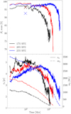 |
Fig. 2 F1 score of ML models tested on N-body simulation data with different SFEs as a function of time (top panel). The half-mass radius (solid lines) and Jacobi mass (dashed lines) are shown in the bottom panel. |
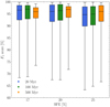 |
Fig. 3 Box plots of F1 score as a function of SFE for different snapshots. The x-axis shows the SFE value of the training set. The color represents the snapshot time of the training sets. Each box plot shows the median, quantiles, minimum, and maximum values of the classification results on more than 1096 synthetic cluster datasets. |
Classification results of the RF model with the Galactic field stars.
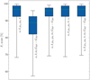 |
Fig. 4 Box plots of F1 accuracy score for the five different parameter combinations used in the training set. |
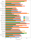 |
Fig. 5 F1 score accuracies for 21 different clusters. Instances with the same training and testing set are dropped. |
3.2 Tests on observational data
We applied our ML approach to the clusters from the Gaia data. As mentioned, we trained on four different models (default set of N-body simulation, Blanco 1, Pleiades, and the NGC 2516 clusters) and then tested it on 21 Gaia clusters. Figure 5 shows the F1 score for all training and testing data combinations. In the following, we first discuss the impact of the training data and then the impact of the testing data.
The models trained on N-body simulation, Blanco 1, the Pleiades, and the NGC 2516 clusters yield average F1 scores1 of 61.4, 51.4, 33.0, and 60.8%, as summarized in Table 4. The highest accuracy of ≈91.1% is reached when the model trained on NGC 2516 was tested on NGC 3532. The lowest accuracy of F1 ⩽ 1% is reached when models trained on Blanco 1 and the Pleiades were tested on IC 4756. Field stars are misclassified as 22 296 and 11408 FPs for these two models.
We analyzed the impact of the quantitative properties of the training sets on the classification accuracy. Table 4 provides the mean F1 scores averaged over Gaia data for models trained on N-body simulation, Blanco 1, the Pleiades, and the NGC 2516 clusters. No clear dependence between the accuracy and the training set mass, age, and rh is apparent. However, the mean F1 score tends to be higher in the models trained on clusters with more member stars, but the dependence is not monotonic.
Figure 6 shows the scatter plots of the F1 score for different clusters as a function of the age (left panel), total mass (middle panel), and half-mass radius (right panel). We do not observe any clear correlation between the F1 score and these quantities. The model trained on the Pleiades cluster exhibits an overall lower accuracy than other models. This is consistent with the lowest average F1 score of 31.4% mentioned above.
As an example of the classification, Fig. 7 shows the histograms of parallaxes for the Blanco 1 cluster. We applied the model trained on N-body simulation (left panel) and Pleiades (right panel). The histograms of different colors represent TPs, TNs, FPs, and FNs according to the key. Overall, the two methods yield similar results. The accuracy is ≈79.0% and ≈71.0% for models trained on N-body simulations and the Pleiades. For the former model, the number of TPs is 501 and that of FNs is 202. For the latter model, we have 424 TPs and 279 FNs.
The reason for this behavior can be identified by considering individual stars. Figure 8 shows the FPs, FNs, and TPs with colorful dots as indicated in the figure key for individual stars as a function of coordinates α and δ (top panels), proper motions in α and δ (middle panels), and magnitudes (bottom panels). The left panel shows a model trained on N-body simulation, and the right panel shows a model trained on the Pleiades cluster. The TP stars of the model trained on the N-body appear to be closer to the center than the TPs of the model trained on the Pleiades. This is visible in the top and middle panels. The locations of FP stars are different in the top and middle panels. FPs are mainly located near the cluster center for the model trained on N-body simulations. However, the FPs are primarily located outside the cluster for the model trained on the Pleiades. FNs appear in similar locations, but there are more FNs for models trained on the Pleiades inside the cluster in the top and middle panels. The bottom panels show that most FPs and FNs of both models are low-mass (dim and cold) stars in the bottom right part of the plot.
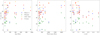 |
Fig. 6 F1 score as a function of age, mass, half mass radius, and density. The different colors correspond to models trained with Blanco 1, the Pleiades, NGC 2516, and N-body simulations. Individual dots correspond to the result of testing on clusters from the Gaia data. |
Characteristics of the training sets and the values of the F1 scores.
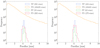 |
Fig. 7 Classification results in terms of parallaxes for the models trained on N-body simulation (left panels) and the Pleiades (right panel) and tested on the Praesepe cluster. |
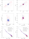 |
Fig. 8 Classification results for individual stars for the models trained on N-body simulation (left panels) and the Pleiades (right panel) and tested on the Praesepe cluster. The top panel shows coordinates α and δ. The middle panels show proper motions in α and δ. The bottom panels show apparent magnitude and color. Due to their large number, the true negatives are not visualized in these plots. |
3.3 Comparison with other methods
We compared the membership derived from our approach to that from the non-ML method of Röser & Schilbach (2019), which is based on a modified convergent-point method. At the same time, we also compared it to the membership from Pang et al. (2022), who used the unsupervised ML method StarGo. We chose the Praesepe cluster as an example to carry out the comparison. We used stars within the same field of view as in the previous sections (see Sect. 2). Of the 1393 member stars from Röser & Schilbach (2019), 1079 lie in this field of view. The stars outside the selected field of view are considered as the tidal tail of Praesepe.
We display the Venn diagram of the comparison of the three methods in Fig. 9. The blue circle corresponds to our method, and the red and gray circles represent the members of Pang et al. (2022) and Röser & Schilbach (2019), respectively. Our method identifies 799 stars as members of Praesepe, while Pang et al. (2022) and Röser & Schilbach (2019) identified 982 and 1079 member stars, respectively. Among all stars, 645 are crossmatched in all three memberships. Seventy stars are identified as members that are not recognized by the other two methods. Two hundred and ten members identified in Röser & Schilbach (2019) are not recovered in the other two methods, most of which are located in the extended tidal tails.
Figure 10 shows color-magnitude diagrams (CMDs) for the member stars identified by these three methods. All three show similar patterns. Our method identifies more faint stars with low effective temperatures because we did not apply a quality cut to the stars before membership identification. These faint stars have larger observational uncertainties than most of the other stars.
The left panel of Fig. 11 displays the distribution of stars by the proper motions in α and δ. Members from our method are very concentrated around μδ ≈ −12 and μα ≈ 35 mass/yr within a radius of ≈4 mass/yr. Members of Pang et al. (2022) are more extended than this region roughly within a radius of ≈5 mass/yr. The members identified by Röser & Schilbach (2019) are distributed most widely, well outside (≳ 10 mass/yr) of the proper motion center. This is consistent with the radial distribution shown in the middle panel of Fig. 11: 4 member stars identified by our method are located farther away than 15 pc from the cluster center, while of the Pang et al. (2022) and Röser & Schilbach (2019) members, 73 and 194 stars lie more than 15 pc away from the cluster center. Similarly, the parallax distribution (right panel of Fig. 11) reveals that the member star identified by our method is confined to a central concentrated region. The main reason for this difference stems from the fact that our method uses the proper motion and parallax for the training.
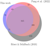 |
Fig. 9 Venn diagram of the comparison of three membership identification methods. Blue corresponds to our method, and gray and red correspond to Röser & Schilbach (2019) and Pang et al. (2022), respectively. |
4 Conclusion
We performed a membership analysis of stellar clusters using a supervised ML algorithm. We trained and tested our models on snapshots data from N-body simulations of stellar clusters and observed clusters from the Gaia DR3 data. Our findings are summarized below.
We studied five supervised ML algorithms on N-body simulation data. These models are RF, DT, SVM, FFNN, and KNN. All models produced comparable accuracies within ≈1% (see Appendix A). Following this result, we used the RF method for the rest of the paper.
We then explored the impact of eight different observational parameters on the accuracy of the membership identification. Five of these eight were astrometric parameters: right ascension (α), declination (δ), proper motions in α (μα) and δ (μδ), and parallax (π), and two were photometric parameters: apparent magnitude m, and color parameter Gbp − Grp. The radial velocity was the last parameter. It is measured with spectroscopy. We tested five different combinations of these eight parameters. The highest accuracy was observed in models trained on purely astrometric parameters α, δ, μα, μδ, and π. The parallax is the most critical parameter in a member classification. The inclusion of rv and photometric features do not seem to improve accuracy. However, this might be biased by the current observational uncertainty of rv.
We studied the impact of the SFE and the cluster age on the classification accuracy using N-body simulation data. The F1 score accuracy, which defines the reliability of our ML method, is ≳90% in all snapshots before cluster dissolution. When the cluster is mainly dissolved, the F1 score accuracy drops to ≈70%. The errors in classification during the dissolution are primarily due to FNs. The statistical results of three snapshots of different SFEs at different times show that the accuracy is similar regardless of the time and SFE of the snapshot used for training.
Additionally, we explored the impact of the number of member and nonmember stars in datasets. Generally, for the successful performance of the supervised ML models, it is desirable to have a similar number of samples in all the classes. The datasets of OCs typically contain a large number of field stars that are not members. We found that the number of field stars within the training dataset does not affect the classification accuracy.
We applied our model to 21 clusters from the Gaia DR3 data. These clusters are Blanco 1, Collinder 69, Huluwa 3, IC 4756, LP 2373 gp2, LP 2373 gp4, LP 2383, LP 2442, Mamajek 4, NGC 1980, NGC 2422, NGC 2451B, NGC 2516, NGC 3532, NGC 6405, NGC 6475, NGC 6633, the Pleiades, Praesepe, Stephenson 1, and UBC 31. In addition to N-body simulation data, we trained our model on Blanco 1, the Pleiades, and the NGC 2516 clusters. The models trained on N-body simulation and NGC 2516 yield an average F1 of ≈60%. The models trained on Blanco 1 and the Pleiades show a lower average F1 score of ≈51% and ≈32%. The models trained on clusters (trained on NGC 2516 and N-body simulation) with a larger number of member stars tend to yield a higher classification accuracy, but the dependence is not monotonic. The two models with the highest accuracy have over 2000 member stars in the training set. In contrast, the two models with the lowest accuracy (trained on Blanco 1 and the Pleiades) have fewer than 2000 members. Among these clusters, we find no noticeable correlation between the classification accuracy and the mass, age, and half-mass radius (rh) of clusters.
We compared our membership determination results with the membership of Pang et al. (2022) and Röser & Schilbach (2019) for the Praesepe cluster. In total, 645 member stars were crossmatched in all three methods. Our model retrieved 124 and 280 fewer stars than Pang et al. (2020) and Röser & Schilbach (2019), respectively. The members identified by our method are more concentrated in both space distribution and proper motion distribution than in the other two methods. Our models were trained on a five-parameter space: right accession, declination, parallax, and proper motions. Therefore, parallax and proper motion play roles that place a greater weight on member identification.
Our work suggests that ML approaches are promising for a membership analysis despite several limitations. We used a limited number of 21 Gaia clusters. The inclusion of more clusters should improve the accuracy. It is also worthwhile to compare the unsupervised learning approach with other ML methods (e.g., StarGO, DBSCAN, HDBSCAN, or GMMs). Moreover, cross-matching the results with other studies of a membership analysis can further improve the results. These limitations will be addressed in future studies.
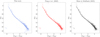 |
Fig. 10 Comparison of three membership identifications in the color-magnitude diagrams. |
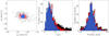 |
Fig. 11 Comparison of three membership labels in terms of proper motions in α and δ (left panel), radial distribution (middle panel), and parallaxes (right panel). Blue, red, and black represent the member stars identified by our method, Pang et al. (2022), and Röser & Schilbach (2019), respectively. |
Acknowledgements
The authors would like to thank the anonymous referee for his/her valuable comments and suggestions, which have helped to improve the quality of this manuscript. This research has been funded by the Science Committee of the Ministry of Education and Science, Republic of Kazakhstan (Grant No. AP13067834, AP19677351, and Program No. BR20280974). Additionally, funding is provided through the Nazarbayev University Faculty Development Competitive Research Grant Program, with Grant No. 11022021FD2912. Xiaoying Pang acknowledges the financial support of the National Natural Science Foundation of China through grants 12173029 and 12233013. Peter Berczik thanks the support from the special program of the Polish Academy of Sciences and the US National Academy of Sciences under the Long-term program to support the Ukrainian research teams grant No. PAN.BFB.S.BWZ.329.022.2023. The data used in this study can be obtained from the authors upon request.
Appendix A Dependence on the ML model
In this section, we check how our results depend on the ML model. We applied RF, DT, SVM, FFNN, and KNN models.
Figure A.1 shows the F1 score as a function of time for different SFE values and different ML models. The colored lines represent F1 score accuracy as a function of time for the RF, DT, SVM, FFNN, and KNN models. The training is performed on N-body simulation snapshots at 20 Myr. All ML models exhibit similar F1 scores. The difference between different models does not exceed ≈1%. The RF model performs slightly better within this difference, especially for t ≲ 200 Myr. We thus adopted the RF model in the main part of our work.
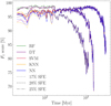 |
Fig. A.1 Average F1 score as a function of time for different ML models. |
References
- Agarwal, M., Rao, K. K., Vaidya, K., & Bhattacharya, S. 2021, MNRAS, 502, 2582 [CrossRef] [Google Scholar]
- Ascenso, J., Alves, J., & Lago, M. T. V. T. 2009, A&A, 495, 147 [NASA ADS] [CrossRef] [EDP Sciences] [Google Scholar]
- Astropy Collaboration (Robitaille, T. P., et al.) 2013, A&A, 558, A33 [NASA ADS] [CrossRef] [EDP Sciences] [Google Scholar]
- Bação, F., Lobo, V., & Painho, M. 2005, in Computational Science-ICCS 2005: 5th International Conference, Atlanta, GA, USA, May 22–25, 2005, Proceedings, Part III 5, Springer, 476 [Google Scholar]
- Bebis, G., & Georgiopoulos, M. 1994, IEEE Potentials, 13, 27 [CrossRef] [Google Scholar]
- Bishop, C. M. 2006, Pattern Recognition and Machine Learning (Springer) [Google Scholar]
- Bland-Hawthorn, J., & Gerhard, O. 2016, ARA&A, 54, 529 [Google Scholar]
- Bouma, L. G., Curtis, J. L., Hartman, J. D., Winn, J. N., & Bakos, G. Á. 2021, AJ, 162, 197 [NASA ADS] [CrossRef] [Google Scholar]
- Breiman, L. 2001, Mach. Learn., 45, 5 [Google Scholar]
- Breiman, L., Friedman, J., Olshen, R., & Stone, C. 1984, Classification and Regression Trees (Chapman and Hall/CRC) [Google Scholar]
- Campello, R. J. G. B., Moulavi, D., & Sander, J. 2013, in Advances in Knowledge Discovery and Data Mining, eds. J. Pei, V. S. Tseng, L. Cao, H. Motoda, & G. Xu (Berlin, Heidelberg: Springer Berlin Heidelberg), 160 [Google Scholar]
- Cantat-Gaudin, T., Jordi, C., Vallenari, A., et al. 2018, A&A, 618, A93 [NASA ADS] [CrossRef] [EDP Sciences] [Google Scholar]
- Cantat-Gaudin, T., Anders, F., Castro-Ginard, A., et al. 2020, A&A, 640, A1 [NASA ADS] [CrossRef] [EDP Sciences] [Google Scholar]
- Castro-Ginard, A., Jordi, C., Luri, X., et al. 2020, A&A, 635, A45 [NASA ADS] [CrossRef] [EDP Sciences] [Google Scholar]
- Chen, L., Hou, J. L., & Wang, J. J. 2003, AJ, 125, 1397 [NASA ADS] [CrossRef] [Google Scholar]
- Chen, Y., Girardi, L., Fu, X., et al. 2019, A&A, 632, A105 [EDP Sciences] [Google Scholar]
- Conrad, C., Scholz, R. D., Kharchenko, N. V., et al. 2017, A&A, 600, A106 [NASA ADS] [CrossRef] [EDP Sciences] [Google Scholar]
- Cortes, C., & Vapnik, V. 1995, Mach. Learn., 20, 273 [Google Scholar]
- Cover, T. M., & Hart, P. E. 1967, Inform. Theory IEEE Trans., 13, 21 [CrossRef] [Google Scholar]
- Das, S. R., Gupta, S., Prakash, P., Samal, M., & Jose, J. 2023, ApJ, 948, 7 [NASA ADS] [CrossRef] [Google Scholar]
- Deb, S., Baruah, A., & Kumar, S. 2022, MNRAS, 515, 4685 [NASA ADS] [CrossRef] [Google Scholar]
- de la Fuente Marcos, R., & de la Fuente Marcos, C. 2004, New A, 9, 475 [NASA ADS] [CrossRef] [Google Scholar]
- Dias, W. S., Monteiro, H., Caetano, T. C., et al. 2014, A&A, 564, A79 [NASA ADS] [CrossRef] [EDP Sciences] [Google Scholar]
- Ester, M., Kriegel, H.-P., Sander, J., & Xu, X. 1996, in Proceedings of the Second International Conference on Knowledge Discovery and Data Mining (KDD) (ACM), 226 [Google Scholar]
- Fürnkranz, J. 2010, Decision Tree, eds. C. Sammut, & G. I. Webb (Boston, MA: Springer US), 263 [Google Scholar]
- Gaia Collaboration (Brown, A. G. A., et al.) 2016a, A&A, 595, A2 [NASA ADS] [CrossRef] [EDP Sciences] [Google Scholar]
- Gaia Collaboration (Prusti, T., et al.) 2016b, A&A, 595, A1 [NASA ADS] [CrossRef] [EDP Sciences] [Google Scholar]
- Gaia Collaboration (Brown, A. G. A., et al.) 2018, A&A, 616, A1 [NASA ADS] [CrossRef] [EDP Sciences] [Google Scholar]
- Gaia Collaboration (Brown, A. G. A., et al.) 2021, A&A, 649, A1 [NASA ADS] [CrossRef] [EDP Sciences] [Google Scholar]
- Gaia Collaboration (Vallenari, A., et al.) 2023, A&A, 674, A1 [NASA ADS] [CrossRef] [EDP Sciences] [Google Scholar]
- Gao, X.-H. 2014, Res. Astron. Astrophys., 14, 159 [CrossRef] [Google Scholar]
- Gao, X. 2018a, ApJ, 869, 9 [NASA ADS] [CrossRef] [Google Scholar]
- Gao, X.-H. 2018b, Ap&SS, 363, 232 [NASA ADS] [CrossRef] [Google Scholar]
- Gao, X.-h. 2019a, PASP, 131, 044101 [NASA ADS] [CrossRef] [Google Scholar]
- Gao, X.-h. 2019b, MNRAS, 486, 5405 [NASA ADS] [CrossRef] [Google Scholar]
- Ghosh, E. M., Sulistiyowati, Tucio, P., & Fajrin, M. 2022, J. Phys. Conf. Ser., 2214, 012009 [NASA ADS] [CrossRef] [Google Scholar]
- Goutte, C., & Gaussier, E. 2005, in Lecture Notes in Computer Science, 3408, 345 [Google Scholar]
- Guido, R. M. D., Tucio, P. B., Kalaw, J. B., & Geraldo, L. E. 2023, in IOP Conference Series: Earth and Environmental Science, 1167, 012010 [NASA ADS] [CrossRef] [Google Scholar]
- Hunt, E. L., & Reffert, S. 2021, A&A, 646, A104 [NASA ADS] [CrossRef] [EDP Sciences] [Google Scholar]
- Hunt, E. L., & Reffert, S. 2023, A&A, 673, A114 [NASA ADS] [CrossRef] [EDP Sciences] [Google Scholar]
- Jadhav, V. V., Pennock, C. M., Subramaniam, A., Sagar, R., & Nayak, P. K. 2021, MNRAS, 503, 236 [NASA ADS] [CrossRef] [Google Scholar]
- Jaehnig, K., Bird, J., & Holley-Bockelmann, K. 2021, ApJ, 923, 129 [NASA ADS] [CrossRef] [Google Scholar]
- Just, A., Berczik, P., Petrov, M. I., & Ernst, A. 2009, MNRAS, 392, 969 [Google Scholar]
- Kalambay, M. T., Naurzbayeva, A. Z., Otebay, A. B., et al. 2022, Recent Contrib. Phys., 83, 4 [Google Scholar]
- Kharchenko, N. V., Piskunov, A. E., Röser, S., Schilbach, E., & Scholz, R. D. 2005, A&A, 438, 1163 [NASA ADS] [CrossRef] [EDP Sciences] [Google Scholar]
- Kharchenko, N. V., Piskunov, A. E., Schilbach, E., Röser, S., & Scholz, R. D. 2012, A&A, 543, A156 [NASA ADS] [CrossRef] [EDP Sciences] [Google Scholar]
- Kohl, M. 2012, Int. J. Statist. Med. Res., 1, 79 [CrossRef] [Google Scholar]
- Kounkel, M., & Covey, K. 2019, AJ, 158, 122 [Google Scholar]
- Krone-Martins, A., & Moitinho, A. 2015, ascl:1504.001 [Google Scholar]
- Krumholz, M. R., McKee, C. F., & Bland-Hawthorn, J. 2019, ARA&A, 57, 227 [NASA ADS] [CrossRef] [Google Scholar]
- Lada, C. J., & Lada, E. A. 2003, ARA&A, 41, 57 [Google Scholar]
- Liu, L., & Pang, X. 2019, ApJS, 245, 32 [NASA ADS] [CrossRef] [Google Scholar]
- Lodieu, N., Pérez-Garrido, A., Smart, R. L., & Silvotti, R. 2019, A&A, 628, A66 [NASA ADS] [CrossRef] [EDP Sciences] [Google Scholar]
- Mahmudunnobe, M., Hasan, P., Raja, M., & Hasan, S. N. 2021, Eur. Phys. J. Special Top., 230, 2177 [NASA ADS] [CrossRef] [Google Scholar]
- Maíz Apellániz, J., & Weiler, M. 2018, A&A, 619, A180 [Google Scholar]
- Meingast, S., & Alves, J. 2019, A&A, 621, A3 [Google Scholar]
- Meingast, S., Alves, J., & Rottensteiner, A. 2021, A&A, 645, A84 [NASA ADS] [CrossRef] [EDP Sciences] [Google Scholar]
- Noormohammadi, M., Khakian Ghomi, M., & Haghi, H. 2023, MNRAS, 523, 3538 [NASA ADS] [CrossRef] [Google Scholar]
- Olivares, J., Lodieu, N., Béjar, V. J. S., et al. 2023, A&A, 675, A28 [NASA ADS] [CrossRef] [EDP Sciences] [Google Scholar]
- Pang, X., Li, Y., Tang, S.-Y., Pasquato, M., & Kouwenhoven, M. B. N. 2020, ApJ, 900, L4 [NASA ADS] [CrossRef] [Google Scholar]
- Pang, X., Tang, S.-Y., Li, Y., et al. 2022, ApJ, 931, 156 [NASA ADS] [CrossRef] [Google Scholar]
- Pang, X., Liao, S., Li, J., et al. 2024, ApJ, 966, 169 [Google Scholar]
- Parmentier, G., & Pfalzner, S. 2013, in Protostars and Planets VI Posters [Google Scholar]
- Paszke, A., Gross, S., Massa, F., et al. 2019, in Advances in Neural Information Processing Systems 32, eds. H. Wallach, H. Larochelle, A. Beygelzimer, F. d’Alché-Buc, E. Fox, & R. Garnett (Curran Associates, Inc.), 8024 [Google Scholar]
- Pedregosa, F., Varoquaux, G., Gramfort, A., et al. 2011, J. Mach. Learn. Res., 12, 2825 [Google Scholar]
- Pera, M. S., Perren, G. I., Moitinho, A., Navone, H. D., & Vazquez, R. A. 2021, A&A, 650, A109 [NASA ADS] [CrossRef] [EDP Sciences] [Google Scholar]
- Peterson, L. E. 2009, Scholarpedia, 4, 1883 [CrossRef] [Google Scholar]
- Phelps, R. L., & Janes, K. A. 1994, ApJS, 90, 31 [NASA ADS] [CrossRef] [Google Scholar]
- Portegies Zwart, S. F., McMillan, S. L. W., & Gieles, M. 2010, ARA&A, 48, 431 [NASA ADS] [CrossRef] [Google Scholar]
- Renaud, F. 2018, New A Rev., 81, 1 [CrossRef] [Google Scholar]
- Röser, S., & Schilbach, E. 2019, A&A, 627, A4 [NASA ADS] [CrossRef] [EDP Sciences] [Google Scholar]
- Röser, S., Schilbach, E., & Goldman, B. 2019, A&A, 621, A2 [NASA ADS] [CrossRef] [EDP Sciences] [Google Scholar]
- Ruprecht, J., Balázs, B., & White, R. E. 1981, Akad. Kiado, 0 [Google Scholar]
- Rybizki, J. 2019, Galaxia_wrap: Galaxia wrapper for generating mock stellar surveys, Astrophysics Source Code Library, record ascl:1901.005 [Google Scholar]
- Sharma, S., Bland-Hawthorn, J., Johnston, K. V., & Binney, J. 2011, ApJ, 730, 3 [NASA ADS] [CrossRef] [Google Scholar]
- Shukirgaliyev, B., Parmentier, G., Berczik, P., & Just, A. 2017, A&A, 605, A119 [NASA ADS] [CrossRef] [EDP Sciences] [Google Scholar]
- Shukirgaliyev, B., Otebay, A., Just, A., et al. 2019, Reports of NAS RK. Physicomathematical series, 130 [Google Scholar]
- Shukirgaliyev, B., Otebay, A., Sobolenko, M., et al. 2021, A&A, 654, A53 [NASA ADS] [CrossRef] [EDP Sciences] [Google Scholar]
- Sindhu Meena, K., & Suriya, S. 2020, in Proceedings of International Conference on Artificial Intelligence, Smart Grid and Smart City Applications, eds. L. A. Kumar, L. S. Jayashree, & R. Manimegalai (Cham: Springer International Publishing), 627 [CrossRef] [Google Scholar]
- Stock, J. 1956, ApJ, 123, 258 [NASA ADS] [CrossRef] [Google Scholar]
- Tang, S.-Y., Pang, X., Yuan, Z., et al. 2019, ApJ, 877, 12 [Google Scholar]
- Tucio, P. B., Guido, R. M. D., & Kalaw, J. B. 2023, IOP Conf. Ser.: Earth Environ. Sci., 1167, 012002 [NASA ADS] [CrossRef] [Google Scholar]
- van Groeningen, M. G. J., Castro-Ginard, A., Brown, A. G. A., Casamiquela, L., & Jordi, C. 2023, A&A, 675, A68 [NASA ADS] [CrossRef] [EDP Sciences] [Google Scholar]
- Yuan, Z., Chang, J., Banerjee, P., et al. 2018, ApJ, 863, 26 [NASA ADS] [CrossRef] [Google Scholar]
All Tables
Confusion matrix representing the performance of the prediction compared to the actual value.
All Figures
|
Fig. 1 Stars from N-body simulation with an SFE of 17% in a 20 Myr snapshot with generated field stars projected onto the sky. The blue, orange, and gray points show the member, nonmember, and Galactic field stars. |
| In the text | |
|
Fig. 2 F1 score of ML models tested on N-body simulation data with different SFEs as a function of time (top panel). The half-mass radius (solid lines) and Jacobi mass (dashed lines) are shown in the bottom panel. |
| In the text | |
|
Fig. 3 Box plots of F1 score as a function of SFE for different snapshots. The x-axis shows the SFE value of the training set. The color represents the snapshot time of the training sets. Each box plot shows the median, quantiles, minimum, and maximum values of the classification results on more than 1096 synthetic cluster datasets. |
| In the text | |
|
Fig. 4 Box plots of F1 accuracy score for the five different parameter combinations used in the training set. |
| In the text | |
|
Fig. 5 F1 score accuracies for 21 different clusters. Instances with the same training and testing set are dropped. |
| In the text | |
|
Fig. 6 F1 score as a function of age, mass, half mass radius, and density. The different colors correspond to models trained with Blanco 1, the Pleiades, NGC 2516, and N-body simulations. Individual dots correspond to the result of testing on clusters from the Gaia data. |
| In the text | |
|
Fig. 7 Classification results in terms of parallaxes for the models trained on N-body simulation (left panels) and the Pleiades (right panel) and tested on the Praesepe cluster. |
| In the text | |
|
Fig. 8 Classification results for individual stars for the models trained on N-body simulation (left panels) and the Pleiades (right panel) and tested on the Praesepe cluster. The top panel shows coordinates α and δ. The middle panels show proper motions in α and δ. The bottom panels show apparent magnitude and color. Due to their large number, the true negatives are not visualized in these plots. |
| In the text | |
|
Fig. 9 Venn diagram of the comparison of three membership identification methods. Blue corresponds to our method, and gray and red correspond to Röser & Schilbach (2019) and Pang et al. (2022), respectively. |
| In the text | |
|
Fig. 10 Comparison of three membership identifications in the color-magnitude diagrams. |
| In the text | |
|
Fig. 11 Comparison of three membership labels in terms of proper motions in α and δ (left panel), radial distribution (middle panel), and parallaxes (right panel). Blue, red, and black represent the member stars identified by our method, Pang et al. (2022), and Röser & Schilbach (2019), respectively. |
| In the text | |
|
Fig. A.1 Average F1 score as a function of time for different ML models. |
| In the text | |
Current usage metrics show cumulative count of Article Views (full-text article views including HTML views, PDF and ePub downloads, according to the available data) and Abstracts Views on Vision4Press platform.
Data correspond to usage on the plateform after 2015. The current usage metrics is available 48-96 hours after online publication and is updated daily on week days.
Initial download of the metrics may take a while.