| Issue |
A&A
Volume 695, March 2025
|
|
|---|---|---|
| Article Number | A271 | |
| Number of page(s) | 14 | |
| Section | Interstellar and circumstellar matter | |
| DOI | https://doi.org/10.1051/0004-6361/202449717 | |
| Published online | 27 March 2025 | |
The bright, dusty aftermath of giant eruptions and H-rich supernovae
Late interaction of supernova shocks and dusty circumstellar shells created by 45, 50, and 60 M⊙ stars
1
Instituto Nacional de Astrofísica Óptica y Electrónica,
AP 51,
72000
Puebla, Mexico
2
Astronomical Institute of the Czech Academy of Sciences,
Boční II 1401/1,
141 00
Praha 4, Czech Republic
★ Corresponding author; This email address is being protected from spambots. You need JavaScript enabled to view it.
Received:
24
February
2024
Accepted:
12
February
2025
Abstract
Context. The late-stage evolution of massive stars is marked by periods of intense instability as they transit towards their final corecollapse. Within these periods, stellar eruptions stand out due to their hallmark of exceptionally high mass-loss rates, resulting in the formation of copious amounts of dust. However, the survival of these dust grains is threatened by the powerful shock waves generated when the progenitor star explodes as a supernova (SN).
Aims. We aim to assess the impact of selected cases of hydrogen-rich SN explosions from progenitors of 45, 50, and 60 M⊙ on dust grains formed after giant stellar eruptions, exploring late interactions with circumstellar shells that occur a few years to centuries after the eruption.
Methods. We present 3D hydrodynamical simulations that follow the evolution of dust particles in a scenario that includes, for the first time, the progenitor’s stellar wind, a giant stellar eruption, and the eventual SN explosion, while in line with the mass budget prescribed by stellar evolutionary models.
Results. For a standard SN ejecta mass of 10 M⊙, kinetic energy of 1051 erg, and a long 200-year eruption-SN gap, only 25% of the dust mass remains 250 years post-explosion in a spherical circumstellar medium (CSM), and only 2% a century after the explosion in a bipolar CSM. Conversely, a shorter gap of a dozen years preserves 75% of the dust mass after shock-processing for a standard explosion, while this drops to 20% for more massive (15-20 M⊙) ejecta with kinetic energy of 5 × 1051 erg.
Conclusions. The CSM geometry and an early SN remnant transition to a radiative phase impact dust survival. As the shock wave weakens from efficiently converting kinetic energy into thermal radiation (up to half of the injected kinetic energy), there is a greater potential for survival, not only for dust in the CSM but also for SN-condensed dust (due to a weaker SN reverse shock), and pre-existing dust in the ambient ISM. Against expectations, a larger fraction of the dust mass can survive if the SN occurs just a few years after the eruption event.
Key words: hydrodynamics / stars: massive / stars: mass-loss / supernovae: general / stars: winds, outflows / dust, extinction
© The Authors 2025
 Open Access article, published by EDP Sciences, under the terms of the Creative Commons Attribution License (https://creativecommons.org/licenses/by/4.0), which permits unrestricted use, distribution, and reproduction in any medium, provided the original work is properly cited.
This article is published in open access under the Subscribe to Open model. This email address is being protected from spambots. You need JavaScript enabled to view it. to support open access publication.
1 Introduction
Interstellar dust plays a crucial role in the interstellar medium (ISM), influencing various astrophysical processes that impact the gas dynamics, chemistry, and thermodynamics within galaxies. These processes include the formation of molecules, planets, and stars (Draine 2003a, 2011; Tielens 2005). The dust ability to absorb and scatter starlight is most pronounced in UV and optical regimes, while it emits radiation in the infrared regime (Draine 2003b).
The origin and nature of dust in galaxies remain not fully understood, although it is recognized to form in the dense and cold envelopes of evolved stars through their stellar winds, especially stars in the asymptotic giant branch stage, red supergiants, Wolf Rayet stars, and luminous blue variable (LBV) stars (e.g. Todini & Ferrara 2001; Crowther 2003; Massey et al. 2005; Tielens 2005; Dwek 2005; Cherchneff 2013; Smith 2010; Kochanek 2011). Furthermore, the ejecta of core-collapse supernovae (SNe) are also known to have the required conditions to form dust and contribute significantly to the dust budget in the Universe (e.g. Elmegreen 1981; Todini & Ferrara 2001; Dunne et al. 2009; Matsuura et al. 2009; Gall & Hjorth 2018; Sarangi et al. 2018; Kirchschlager et al. 2019, 2020; Priestley et al. 2021, 2022).
During their evolution, stars experience fast outflows that inject mechanical energy, mass, and momentum into the ISM. These outflows, known as stellar winds, lead to the formation of bubbles around the progenitor stars, since the winds are ejected into the ISM at supersonic speeds (Weaver et al. 1977; Dyson 1989; van Marle et al. 2004; Draine 2011). Moreover, massive stars can also lose mass during eruptive processes, which tend to occur when the star becomes unstable as it approaches the so-called Eddington limit (e.g. Humphreys & Davidson 1994). Indeed, when the Eddington limit is reached, the radiation forces at the surface prevail over gravity, resulting in a substantially increased mass-loss rate. These outbursts or stellar eruptions are explosive events during which a huge amount of gas is ejected from the star’s surface into the surrounding medium. Therefore, they can lead to the creation of intricate shell-like structures and contribute to the enrichment of the ISM with heavy elements that can subsequently condense onto dust particles (Kochanek 2011; Smith 2014). These eruptions can endure for months or even years, leading to the development of a dense circumstellar medium (CSM) surrounding the star (e.g. Smith 2011; Davidson 2020). Previous numerical simulations have successfully modelled the formation and evolution of such CSM structures around massive stars (e.g. Garcia-Segura et al. 1996a,b).
Furthermore, the powerful shock waves generated by corecollapse SNe can dramatically influence the fate of the dust grains formed during the preceding stellar outbursts, as they interact with the pre-existing CSM weeks to centuries postexplosion (Smith & Andrews 2020). The extreme temperatures, pressures, and velocities associated with the shock waves, along with the intense shock breakout radiation, can result in the destruction, fragmentation, or vaporization of the dust grains (e.g. Nozawa et al. 2010; Temim et al. 2015; Gall & Hjorth 2018; Micelotta et al. 2018).
These interactions often involve an asymmetric environment around the progenitor, typical of evolved massive stars, with non- spherical CSM structures like discs or bipolar outflows (Smith et al. 2018; Qin et al. 2024). This asymmetry strongly impacts the observed SNR-CSM interaction signatures and can result in a large amount of radiated energy when the SN blast wave interacts with the dense stellar wind and outburst-produced CSM (van Marle et al. 2010; Pan et al. 2013; Vlasis et al. 2016; Smith 2017; Smith & Andrews 2020; Margalit 2022; Martinez et al. 2024; Bersten et al. 2024).
The best known case of a stellar eruption in the Milky Way is the Great Eruption of η Carinae (η Car) around 1843 that formed its remarkable bipolar nebula known as the Homunculus (Humphreys & Davidson 1994; Mac Low et al. 1996; Davidson & Humphreys 1997). η Car is a luminous binary star system classified as LBV, with two massive components of about 90 M⊙ and 30 M⊙, respectively (Madura et al. 2012). The Great Eruption resulted in the ejection of a massive amount of material; hence, the high density, low temperature, and abundance of heavy elements in the erupted matter provided favourable conditions for the formation of dust particles (Humphreys & Martin 2012; Weis 2012). Indeed, up to 0.4 M⊙ of dust were produced after the eruption (Gomez et al. 2010), raising questions about its fate in the event of a SN explosion (e.g. Gall & Hjorth 2018).
Furthermore, dust formation in SNe showing interaction with a dense CSM has also recently been studied, providing both theoretical and observational evidence of the formation of new dust grains following the collision of the SN blast wave with the dense CSM (Sarangi & Slavin 2022; Smith et al. 2024). Examples of core-collapse SNe exhibiting evidence of strong interaction with a dense CSM include SN 2005gj (Trundle et al. 2008), SN 2005gl (Gal-Yam et al. 2007), SN 2017hcc (Kumar et al. 2019; Smith & Andrews 2020), SN 2005ip (Smith et al. 2017), SN 2015da (Smith et al. 2024), SN 2007od (Andrews et al. 2010), SN 2004et (Szalai et al. 2021), SN 2013ej (Mauerhan et al. 2017; Szalai et al. 2021), and SN 2018lab (Pearson et al. 2023).
The wide range of timescales, from weeks to millennia, between eruptive episodes and subsequent SN explosions, which is highlighted by available data (Brethauer et al. 2022), is an intriguing research subject. This work examines these timescales as crucial parameters influencing the dynamics of these phenomena.
Here, we employ detailed 3D hydrodynamical calculations to investigate the impact of selected cases of hydrogen-rich SN explosions on dust grains formed during late-stage stellar outbursts. Our goal is to determine whether these explosions result in the complete or partial destruction of the circumstellar dust. In particular, we simulate the evolution of the SN blast wave, its interaction with the pre-SN erupted matter and stellar wind, and calculate on the fly the resulting destruction of the erupted dust grains. By comparing the initial and final amount of the dust grains, we quantify the degree of destruction and gain insights into the survival mechanisms of interstellar dust.
The paper is organized as follows. Section 2 describes the implemented hydrodynamical scheme, and the initial conditions for the stellar winds (Sect. 2.1), the erupted CSM evolution (Sect. 2.2), and the supernova remnant (SNR) evolution (Sect. 2.3). In Sect. 3, we present the results of the simulations, and the summary and conclusions are presented in Sect. 5.
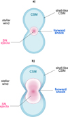 |
Fig. 1 Schematic (not to scale) of a SNR evolving within a bipolar CSM created by a stellar eruption, subsequent to the ejection of the stellar wind. Panel a shows the expansion of the SN ejecta and the forward shock at early times after the explosion. Panel b presents the time when the SN begins to interact with the densest medium left by the eruption. |
2 Numerical set-up
Figure 1 presents a schematic illustration of the late-stage evolution of a massive star undergoing several mass-loss episodes. First, the fast stellar wind from the star continuously injects mass and energy into the ambient ISM gas. Later, the star goes through an eruptive episode that creates a bipolar CSM (shown in the scheme as blue). Finally, the star explodes as SN, expanding into the CSM (panel a). The SN forward shock eventually collides with the densest sections of the erupted matter (panel b), first towards the equator and later with the poles of the structure.
Stellar winds may be inhomogeneous, which leads to a reduction in the empirical mass-loss rates (Oskinova et al. 2007). Therefore, we estimated the characteristic cooling timescale in the free wind regions (see Eq. (A.11)) and found that in all our models, it is much longer than our simulation timescales. However, it depends on the injection radius, Rw, which we cannot decrease significantly. Another important issue is the potential impact of numerical diffusion, which can suppress or limit the growth of thermal instabilities.
Therefore, we have carried out a set of 3D hydrodynamical simulations using the adaptive-mesh refinement (AMR) code FLASH 4.6 (Fryxell et al. 2000). The code implements the piece-wise parabolic method to solve the hydrodynamic equations (Colella & Woodward 1984). The package PARAMESH (MacNeice et al. 1999) was used to implement the AMR grid, which employs a block-structured adaptive mesh refinement scheme.
The simulation scheme includes the calculation of a timedependent stellar wind (Sect. 2.1) and the SN explosion (Sect. 2.3) using the Wind module (Wünsch et al. 2008, 2017), which was also adapted to allow for the injection of the stellar eruption (Sect. 2.2). Furthermore, we also included radiative cooling at solar metallicity, as was prescribed by Schure et al. (2009), assuming collisional ionization equilibrium and instantaneous electron-ion energy equipartition. In our case, the validity of these assumptions stems from the high densities and short timescales characterizing the region behind the forward shock, where the bulk of radiative cooling occurs (Spitzer 1962; Smith & Hughes 2010; Wong et al. 2016). The implementation also includes the injection and destruction of dust particles, and the additional radiative cooling resulting from gas-grain collisions, calculated on the fly with the CINDER module (Cooling INduced by Dust & Erosion Rates, Martínez-González et al. 2018, 2019, 2022).
In our calculations, we assume three progenitor stars with masses of 45, 50, and 60 M⊙ at the zero-age main sequence (ZAMS). The first two progenitors are assumed to have formed with a metalliciy of 0.02 Z⊙, whereas the third is assumed to have formed with the Milky Way’s metalliciy of 0.73 Z⊙. According to the Bonn Optimized Stellar Tracks (BoOST Szécsi et al. 2022), such stars evolve over to the point of forming a carbon core. This phase is reached when each star is about 99% through their lifetime, having shed a substantial amount of mass through a stellar wind. Despite this loss, the 45-M⊙, 50-M⊙, and 60-M⊙ stars still maintain a mass of ~42.5, 47, and 37 M⊙, respectively. In the remaining 1% of the stars’ lifetime, we assume the occurrence of a giant stellar eruption, shedding ~25 M⊙ of material (e.g. Woosley et al. 2007; Smith et al. 2010; Wang et al. 2022). Subsequently, as the stars progress towards their ultimate fate, a hydrogen-rich core-collapse SN occurs (consistent with expectations for carbon core masses below 40 M⊙ Szécsi et al. 2022), ejecting ≥10 M⊙ of material and leaving behind a compact stellar remnant. Hydrogen-rich core-collapse SNe typically yield relatively small amounts of 56Ni (Anderson 2019; Rodríguez et al. 2021). Nevertheless, for energetic hydrogen-rich SNe, a higher 56Ni content is expected, as is exemplified by the SNe iPTF14hls (Wang et al. 2022), and 2006gy (Moriya et al. 2013). We thus also accounted for the impact of radiative heating from the decay of 56Ni in the SNR evolution.
2.1 Stellar winds
An isotropic stellar wind was simulated according to the implementation of Wünsch et al. (2017), in which the wind mass and energy are inserted within a radius, Rw, centred at the origin of the spatial domain. For each grid cell within Rw , mass was first added and the velocity was corrected to ensure momentum conservation. Subsequently, energy was also added according to the wind energy deposition rate. The gas density around the source, within Rw, was set as
 (1)
(1)
and
 (2)
(2)
respectively. In these equations, Ṁw is the time-dependent massloss rate, υ∞ is the wind terminal velocity, and r is the distance from the centre. The wind insertion radius, Rw, was set to be as small as possible, such that the wind is approximately spherical.
The wind temperature, Tw, was set to 104 K, as in Martínez-González et al. (2019). Following Frank et al. (1995); González et al. (2022), our calculations assume that Ṁw = 10−3 M⊙ yr−1, and υ∞ = 250 km s−1 around the time the subsequent eruption occurs. No dust was inserted together with the stellar wind as our aim here is to study the fate of the dust injected by the stellar eruption. The calculations assume solar metallicity (Z = Z⊙).
The stellar wind was left to evolve until it extended beyond the boundaries of the computational domain. Afterwards, the stellar wind was switched off upon the insertion of the stellar eruption.
It is worth noting that the computational cost of the stable stellar wind phase was relatively low compared to the more demanding calculations for the following stages, which include both the stellar eruption and the SNR. This allowed us to include the wind phase in the simulations without significantly increasing the overall computational expense. We would also like to highlight that calculating the wind in 3D directly on the Cartesian grid avoids the potential sources of noise and inaccuracies that could arise from remapping a spherically symmetric wind solution onto a Cartesian grid.
2.2 Erupted CSM evolution
Here, the evolution of the expanding circumstellar matter resulting from a stellar eruption is studied by considering several input parameters, including the deposited kinetic energy, Ek,e, the maximum expansion velocity, υmax,e, and the total mass of the eruption ejecta, Me. Similarly to the stellar wind insertion, the eruption ejecta was modelled by inserting mass and internal energy in all grid cells within an insertion radius during a single time-step. The radius of the inserted eruption, denoted as Re, was limited by the spatial resolution. We minimized the insertion radius to cover the smallest possible volume so the eruption maintains an approximately spherical shape; this ensures minimal error in the mass and energy insertion. We assume that the initial distribution for the ejecta density is given by
 (3)
(3)
where fe(we) is a structure function:
 (4)
(4)
with a power law index of k > 0, we = r/Re, and wsh,e = Rsh,e /Re.
Here, r, Rsh,e, and Re are the distance from the eruption site, and the inner and outer radii of the homogeneous eruption layer, respectively. The terms f0,e and fk are constants set by the mass and energy conservation (see Appendix B).
Figure 2 presents the ejecta density distribution for Re = 0.06 pc, k = 2.5, and wsh,e = 0.95, where one can note that density increases with r up to a defined radius, Rsh,e, followed by an uniform density outer shell between Rsh,e and Re. This approximation for the density distribution is designed to match a thin, hollow CSM shell mass distribution, similar to that observed in the Homunculus Nebula (e.g., Smith 2006, 2017; Smith et al. 2018; Steffen et al. 2014), where the value of wsh,e = 0.95 corresponds to a shell thickness of 5% of Re. We note that similar density profiles to the one given by Eqs. (3) and (4) have been used before to describe the initial conditions of other explosive events, such as SNRs (e.g. Truelove & McKee 1999; Tang & Chevalier 2017).
In order to model the bipolar morphology of the erupted CSM, we assume a latitude-dependent expansion velocity (Smith 2006):
 (5)
(5)
where the radial velocity, υr,e, follows a Hubble-like expansion:
 (6)
(6)
and
 (7)
(7)
is the function introduced by Frank et al. (1995) to describe the angular dependence of the expanding ejecta (see also Blondin et al. 1995). The parameter α controls the pole-to-equator velocity contrast, β controls the shape of the erupted CSM, and ϕ is the azimuth angle. We fixed α and β to 0.78 and 0.3, respectively, in order to obtain a bipolar CSM similar to the Homunculus (González et al. 2004).
The maximum expansion velocity of the eruption ejecta was derived from energy conservation as
![Mathematical equation: ${\v _{\max ,{\rm{e}}}} = {\left[ {\left( {{{2{E_{{\rm{k}},{\rm{e}}}}} \over {{I_e}{M_{\rm{e}}}}}} \right){1 \over {{f_k}{\lambda _\v } + {{{f_{0,{\rm{e}}}}} \over 5}\left( {1 - w_{{\rm{sh}},{\rm{e}}}^5} \right)}}} \right]^{1/2}},$](/articles/aa/full_html/2025/03/aa49717-24/aa49717-24-eq8.png) (8)
(8)
where
 (9)
(9)
and λυ is a constant dependent on the initial conditions (see Appendix B).
In this set-up, we assume that the stellar wind prior to the eruption is spherical, and the bipolar shape results from the eruption itself. However, in Appendix C, we have also explored the opposite scenario, in which the stellar wind is aspherical and the eruption is inserted with spherical symmetry. We demonstrate that both cases lead to similar CSM morphologies by the time the SN explosion occurs.
Since we adopted an eruption ejecta mass of Me = 25 M⊙, with a dust-to-gas mass ratio of ~0.01 (Smith & Ferland 2007), the ejected dust mass from the eruption is Mdust = 0.25 M⊙ in all our models. Furthermore, we assume that the kinetic energy of the eruptions is Ek,e = 1050 erg (Smith et al. 2018; Smith & Andrews 2020) in all cases. Finally, we considered only one eruptive event, acknowledging that massive stars may undergo multiple eruptions throughout the final stages of their evolution (Kochanek 2011).
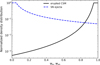 |
Fig. 2 Normalized density distributions of ejected material during the eruption and the SN ejecta expressed as a function of we = r/Re and wsn = r/Rsn, respectively. Note that the CSM follows a shell-like density structure. |
2.3 Supernova remnant evolution
In order to model the SNR evolution, we considered as input parameters the total kinetic energy, Ek,sn, the maximum SN ejecta expansion velocity, υmax,sn, and the total ejected mass, Msn. The insertion of the SNR was performed analogously to the insertion of the erupted CSM. Thus, following Tang & Chevalier (2017) and Truelove & McKee (1999, see also Chevalier 1982), the density distribution is given by
 (10)
(10)
 (11)
(11)
where Rsn is the SNR insertion radius, wsn = r/Rsn, and wc,sn = Rc,sn / Rsn.
We note that SNe follow a decreasing power law density distribution, as is depicted in Fig. 2 for Rsn = 0.04 pc, and wc,sn = 0.05. The index, m, of the power law envelope region was chosen to be equal to 1.
The initial radial velocity of the SN ejecta follows a profile analogous to the one given by Eq. (6) but we also assume that the SN ejecta is initially spherically symmetric. In such a case, energy conservation defines the maximum velocity of the expanding SN ejecta:
![Mathematical equation: $\matrix{ {{\v _{{\rm{max}},{\rm{sn}}}} = {{\left[ {2w_{{\rm{c}},{\rm{sn}}}^{ - 2}\left( {{{5 - m} \over {3 - m}}} \right)\left( {{{w_{{\rm{c}},{\rm{sn}}}^{m - 3} - m/3} \over {w_{{\rm{c}},{\rm{sn}}}^{m - 5} - m/5}}} \right){{{E_{{\rm{k}},{\rm{sn}}}}} \over {{M_{{\rm{sn}}}}}}} \right]}^{1/2}}.} \cr {\rm{}} \cr } $](/articles/aa/full_html/2025/03/aa49717-24/aa49717-24-eq12.png) (12)
(12)
We assume four cases for hydrogen-rich core-collapse SN explosions. In the first one (B12−10), a standard ejecta mass and kinetic energy of 10 M⊙ and 1051 erg (van Marle et al. 2010; Dessart et al. 2016; Matsumoto et al. 2025), respectively, were considered. In the second case (B12−56Ni), we used the same parameters as in the B12−10 case, but with the SN ejecta set at an initial temperature of 106 K aimed to mimic the effect of radioactive decay heating (see Appendix D). In the third case (B12−15), a more massive and energetic explosion is assumed, releasing 15 M⊙ of gas with a kinetic energy of 5 × 1051 erg. This is consistent with SN iPTF14hls, whose estimated energy is between 1051 −1052 erg, and which has an ejecta mass greater than 10 M⊙ (Andrews & Smith 2018; Wang et al. 2022). For the fourth case, an even more massive SN ejecta is assumed, releasing 20 M⊙ of gas with a kinetic energy of 5 × 1051 erg (e.g. the SN 2006gy, Smith et al. 2010; Moriya et al. 2013).
In the latter cases B12−15 and B12−20, we assumed MNi ~ 0.9 M⊙ and 2.5 M⊙, respectively (Wang et al. 2022; Moriya et al. 2013). Thus, the corresponding energies released by the radioactive decay of 56Ni (see Eq. (D.1)) result in ejecta temperatures of >107 K. In the three cases considering the radioactive decay heating, we disabled radiative cooling for the first 200 days of the SNR’s evolution, allowing it to cool solely through adiabatic expansion (although cooling from processes like CO rovibrational transitions should be at play Ono et al. 2024).
As we did for the stellar wind, we refrained from injecting any dust along with the SN ejecta. This allows us to focus on individually tracking the dust originating from the erupted CSM. In doing so, we aim to better understand the fate of CSM-formed dust grains, recognizing the complexity that would arise from attempting to trace dust grains from multiple sources.
Initial conditions.
2.4 Dust injection and destruction
The injection and destruction of dust in the simulations was carried out with the CINDER module, which also allows one to calculate, on the fly, the rate of the thermal sputtering within specific grid cells. CINDER incorporated an initial grain size distribution with 10 bins logarithmically spaced, and the dust was traced by means of the dust-to-gas mass ratio as an advecting mass scalar. The grain sizes follow a log-normal distribution of the form ~a−1 exp{−0.5[ln(a/a0)/σ]2}, where a is the grain size, a0 = 0.1, σ = 0.7, and amin = 0.005 µm, amax = 0.5 µm are the lower and upper limits of the grain size, respectively (see Martínez-González et al. 2018, 2021).
2.5 Initial conditions
Our simulations initialize with a spherical stellar wind that undergoes evolution within an ambient medium of number density n = 1 cm−3 . The presence of this wind sets the conditions for the subsequent evolution of the erupted CSM. The latter was simulated considering different cases with spherical and bipolar (similar to the Homunculus Nebula) geometries. Such an eruption leads to Mdust = 0.25 M⊙ of dust being produced. Finally, the simulations took into account the effects of a spherical SN explosion that interacts with the pre-existing CSM created by the eruption and the stellar wind. Additionally, the growth of dust grains was also included using the capabilities of the CINDER module, as is described in Martínez-González et al. (2022). The simulations incorporate white noise; that is, random initial density perturbations.
We explored three distinct scenarios based on the shape of the erupted CSM, and the eruption-SN gap. For the first and second scenarios, the SN explosion is considered to occur 200 yr after the CSM ejection as a result of the eruptive episode. This time interval aligns with cases such as SN 2004dk and SN 2007od, whose estimated CSM-SN delay time is >100 years (Andrews et al. 2010; Mauerhan et al. 2018), and it is also comparable with the time elapsed from the Great Eruption of η Car to the present day. These two scenarios consider a spherically symmetric CSM (case S200), and a bipolar-shaped CSM (case B200), respectively.
In certain instances, the eruption may occur just a few years prior to the SN explosion, as is exemplified by the SNes 2006qq, 2006Y, 2017hcc, 2018zd, and 2020tlf, whose estimated evolution time is within the range of 6–12 years (Taddia et al. 2013; Smith & Andrews 2020; Hiramatsu et al. 2021a,b; Chugai & Utrobin 2022). Therefore (in cases B12−10, B12−56Ni, B12−15, and B12−20), the SN explosion occurs 12 yr after a bipolar CSM ejection.
Table 1 presents the initial parameters adopted for the stellar wind, the erupted CSM, and the SNR for each case. The simulations in the S200 and B200 cases take place in a cubic computational domain in which the origin of the Cartesian coordinate system lies at the centre, and whose size is (2pc)3 and (1 pc)3 for cases S200 and B200, respectively. In the B12 cases, the simulations were performed in a single octant of the computational domain with size (0.05 pc)3.
A minimum refinement level of 5 and maximum of 71 were considered for S200 and B200, and 6 and 8 for B12−10, B12−56Ni, B12−15, and B12−20. We set the minimum and maximum spatial resolutions shown in Table 1. The external boundary conditions were set to outflow in cases S200 and B200, while in the simulations conducted within a single octant, reflecting boundary conditions were implemented on the planes x = 0, y = 0, and z = 0. Low-resolution convergence tests were also conducted for the S200, B200, and B12−10 cases, with the corresponding minimum and maximum resolutions listed in Table 1.
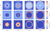 |
Fig. 3 Evolution of the SNR within the erupted CSM for S 200, with each column showing snapshots at tSN = 4,40,170, and 250 yr after the SN explosion, respectively. From top to bottom, each row displays, in log scale, the number gas density, the gas temperature, and the dust mass density. |
3 Results
Figures 3, 4, and 6 present x−z slices of the logarithm of the number gas density, temperature, and dust mass density of four snapshots for S200, B200, and B12−10, respectively. Similarly, Fig. 7 presents the logarithm of the gas temperature only. For the B12−10, B12−15 and B12−20 cases, Figs. 6 and 7 show the plots mirrored along the x and z axes to illustrate the simulations as if they were conducted across the full domain instead of a single octant. Appendix E also presents 1D density profiles along the x and z axes for B200 and B12−10, for the same post-SN times as in Figs. 4 and 6, respectively. Finally, Figs. 5 and 8 show the evolution of the SN kinetic, thermal, and radiated energies, and the dust mass fraction after the SN explosion for all the models listed in Table 1.
3.1 200-year eruption-SN delay
The S200 (spherical) and B200 (bipolar) cases are characterized by a distinct geometry of the CSM created by the eruption. In both cases, the stellar eruption occurs 200 years before the SN explosion. The top left panels in Figs. 3 and 4 show the instant a few years after the SN explosion (tSN = 4 yr), when the shell-like CSM have reached maximum number densities of ~104.5 cm−3 and ~106 cm−3 for S200 and B200, respectively. These densities are lower than those found in the outer shell of the Homunculus Nebula, which average approximately 107 cm−3 (Smith 2006).
For case S200, the SN forward shock initially grows almost in free expansion given the relatively low-density cavity created by the preceding stellar eruption. We note that the kinetic energy (solid line in the top left panel of Fig. 5) decreases slightly and the thermal energy (dashed line) is very small during these early stages (tSN ≲ 170 yr), indicating that the forward shock has indeed processed only a small fraction of the circumstellar gas. On the other hand, the high shock velocity and post-shock temperatures (T ~ 107 K, see the middle row of Fig. 3) lead to an efficient destruction of the CSM dust located in those inner regions, as is shown in the bottom row of Fig. 3. However, the dust mass fraction decreases just ~10% (see the bottom panel of Fig. 5) as only a small amount of dust is located within the cavity. Once the forward shock reaches the densest region of the CSM at tSN ~ 170 yr, the shock processes the largest fraction of dust in the shell, increasing considerably the amount of dust destroyed, as is shown by the steeper decline on the dust mass fraction in the bottom left panel of Fig. 5. After 250 years post-explosion, around 25% of the dust mass (~0.06 M⊙) produced in the erupted CSM still remains. Finally, it is also interesting to note that the middle row in Fig. 3 shows that up to the simulated time, the SN reverse shock has not started moving inwards, which may be due to the still very low thermal energy (and thus thermal pressure) behind the forward shock. In this case, the impact of gas and dust cooling is negligible for the simulated time (see Erad (dotted line) in the top left panel of Fig. 5).
The SNR evolution within the bipolar CSM (case B200) proceeds somewhat differently. First, in this case, the cavity density is larger than in S200 (see the top row in Fig. 4). Also, at tSN = 20 yr the SN forward shock collides with the equatorial section of the CSM shell. Hence, the thermalization of the SN energy proceeds faster. This is shown in the top right panel of Fig. 5, where the SN kinetic energy drops rapidly while being transformed into kinetic and thermal energy of the shocked gas. Furthermore, this is also supported by the fact that, unlike S200, in this case the SN reverse shock starts moving towards the centre (see the middle row in Fig. 4) very early in the evolution of the remnant (tSN ~ 70−100 yr). It becomes increasingly evident that the SNR undergoes deformation, acquiring a configuration that closely resembles the bipolar shape of the CSM, as is depicted in Fig. 4. This suggests that the SNR is constrained from expanding freely in the direction of those sections of the CSM, due to the high equatorial densities.
The lower panels of Fig. 5 show that the dust destruction in B200 occurs more efficiently than in S200. As a result, in the bipolar case only ~2% of the CSM dust survives 115 years post-explosion. However, we argue that the main difference between S200 and B200 regarding the fate of the CSM dust is the timescale of the destruction process, which is smaller in B200 only because the forward shock encounters the bulk of the CSM dust (located in the dense shell) faster than in S200. Ultimately, however, the eruption and SN composite remnant will keep expanding, and the destruction of the CSM dust grains will continue in both cases. Given the similarities to the B200 case, it is expected that in a circumstellar nebula like the Homunculus, all the dust produced after the eruption would be destroyed if the progenitor exploded as a SN.
It should be noted that as soon as the forward shock starts its interaction with the CSM shell, the radiated energy increases considerably (dotted line in the top right panel of Fig. 5). In fact, the remnant thermal energy reaches a peak value of ~0.15ESN at tSN ~ 25 yr, and then starts to fall afterwards, which could delay the reverse shock in its motion towards the explosion centre. This maximum for the gas thermal energy differs considerably with the one expected for an adiabatic SNR (~0.7 ESN). Hence, although gas cooling is not sufficient to decrease the destruction rates of the CSM dust grains in this particular case (B200), it could potentially hinder the ability of the SN forward shock to destroy the interstellar dust contained within the wind-driven shell located at a greater distance at later stages of its evolution (Martínez-González et al. 2019). Finally, between tSN = 50 yr and tSN = 115 yr, one can observe a slight increase in the kinetic energy as the SN shock wave reaches and expands into the decreasing wind density, and therefore it accelerates (e.g. Tenorio-Tagle et al. 2015; Jiménez et al. 2021).
We conducted convergence tests at lower resolution for both the S200 and B200 cases (namely, S200−Test and B200−Test) using a maximum refinement level of 6, obtaining the resolutions shown in Table 1. The results, depicted in Fig. 5 by thin lines, demonstrate an agreement within 1% for the energy and within 2% for the dust mass fraction in S200, and similarly, an agreement within 1% for the energy and 1% for the dust mass fraction for B200.
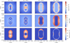 |
Fig. 4 Same as Fig. 3 but for B200, with snapshots at tSN = 4,20,75, and 115 yr, respectively. Additional 1D density profiles along the x and z axes are provided in Appendix E. |
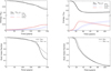 |
Fig. 5 Upper panels: SNR (only gas) kinetic (solid), thermal (dotted), and radiated (dashed) energies as a function of time for S200 (left) and B200 (right). Lower panels: evolution of the dust mass, normalized to that ejected by the eruption. For all panels, thicker lines correspond to S200 and S200, while thinner lines to B200−Test and S200−Test, respectively. |
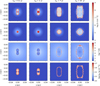 |
Fig. 6 Same as Fig. 4 but for B 12−10, with snapshots at tSN = 0.1,1,7 , and 10 yr after the SN explosion, respectively. Note in the last column that several blisters of shock-heated gas already extend beyond the CSM density distribution. Additional 1D density profiles along the x and z axes are provided in Appendix E. |
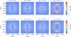 |
Fig. 7 Gas temperature distribution slices in the x−z plane, with the first row showing results for B12−15 and the second row for B12−20. |
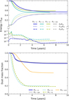 |
Fig. 8 Same as Fig. 5 but for B12−10,B12−56Ni, B12−15, B12−20, and B12−wind (see Appendix C). Note that while the curves corresponding to cases B12−10 and B12−56Ni are presented up to 10 years post-SN, the ones corresponding to B12−15, B12−20, and B12−wind are presented only up to 7–8 years, as the simulations have reached the boundaries of the computational domain, but the most relevant phase of their evolution has already taken place. |
3.2 12-year eruption-SN delay
The B12−10, B12−56Ni, B12−15, and B12−20 models also consider a bipolar CSM but with a 12-year delay between the onset of the stellar eruption and the SN explosion. Due to the short delay time, the CSM cavity is much denser compared to S200 and B200, reaching densities of ~109 cm−3 mostly concentrated at equatorial latitudes (see the top row of Fig. 6). Thus, the shock wave undergoes a rapid transition to a radiative phase, bypassing the Sedov-Taylor phase (Pan et al. 2013).
In the B12−10 case, the solid line in the bottom panel of Fig. 8 shows that although the dust grains begin to be processed soon, by the time the SN reaches the densest region of the CSM (tSN = 1 yr, second column in Fig. 6), dust destruction is limited, and as much as 75% (0.19 M⊙) is preserved.
In the B12−56Ni case, the thermal, kinetic, and radiated energy curves nearly overlap with those of B12−10, appearing as single curves in each plot. Here, about 76% of the dust mass is conserved (thin solid grey line in Fig. 8), slightly higher than in the B12−10 case. This is because the SN shell has a slightly larger thickness (hence, it is less dense) due to the absence of radiative cooling, leading to less dust destruction. We note that as the SN ejecta becomes optically thin to γ-rays around 200 days after the explosion, the radioactive heating efficiency is expected to sharply decrease over time (Matsumoto et al. 2025).
Conversely, for B12−15 and B12−20, where the explosion energy is higher, the SNRs expand more rapidly, reaching the equatorial region of the CSM shell in a shorter time, as is shown in the second column of Fig. 7. Consequently, at tSN = 0.5 yr, the stronger shock induces a more efficient dust destruction, resulting in preserving about 20% of the dust mass (see the dashed and dotted curves in the lower panel of Fig. 8). In all B12 cases – namely, B12−10, B 12−56Ni, B12−15, B12−20 and B12−wind (see Appendix C) – stabilized dust mass fractions have been reached by the end of the simulations, suggesting prolonged survival of the remaining CSM dust grains.
In the case of B12−10, the gas thermal energy remains orders of magnitude lower than the kinetic energy due to the strong gas and dust cooling, as is shown by the dashed and dotted lines in Fig. 8. For cases B12−15 and B12−20, the amount of gas thermal energy is higher, reaching up to 5 × 1050 erg due to the injection of energy via 56Ni radioactive decay heating (see Appendix D). The radiated energy corresponding to case B12−10 reaches values of >0.4 ESN (= 4 × 1050 erg) at tSN = 10 yr, which is comparable with that obtained by van Marle et al. (2010) for their 2D B04 model with similar parameters (a 25 M⊙ CSM shell and a SN explosion injecting 10 M⊙ of gas) for a 2-year eruption-SN gap. On the other hand, for B12−15 and B12−20, the cumulative radiated energy reaches approximately Erad ~ 0.5ESN (equivalent to 2.5 × 1051 erg) after tSN = 7 and tSN = 8 years, respectively. Therefore, it is expected that this energy should be emitted as infrared radiation by shock-heated CSM dust grains (Chevalier & Fransson 2017; Tartaglia et al. 2020; Dwek et al. 2021).
As can be observed in the top and middle panels in Fig. 6, the SN shock wave manages to overrun the whole erupted CSM, leaving a cold region behind. According to Tenorio-Tagle et al. (1990), the mass of a an encompassing dense shell must be approximately 40 times greater than that of the SN ejecta to effectively prevent it being overrun by the SN blast wave. However, in the current scenario, this criterion is far from being fulfilled, as the mass of the erupted CSM is only 2.5 times the SN ejecta mass.
Counterintuitively, our results reveal that for a given SN energy, a shorter delay time between an eruptive episode and the subsequent SN explosion results in a larger fraction of surviving dust mass. This unexpected outcome is attributed to the enhanced radiative cooling as the dusty CSM is still very dense (reaching densities of ~109 cm−3) at its early stages. This result emphasizes the crucial role of the time interval in shaping the fate of dust grains generated after stellar eruptions. It also shows that pre-existing dust grains in the surroundings of SNRs with late CSM interactions have a greater chance of survival.
Finally, the growth of ‘blisters’ of hot gas is observed on the surface of the eruption and SN composite remnant, as is depicted in the middle row of Fig. 6 and in Fig. 7. They are created by the interaction of the SN shock that has passed through the CSM with the slow stellar wind. This is similar to the scenario described by Pittard (2013), except that the hot gas is not escaping from the interior of the CSM shell but generated by the shock on the shell surface. In our model, these features are resolved with 24 grid cells per shell thickness, which corresponds to a shell thickness of 0.00152 pc within a spatial domain of (0.05 pc)3. By contrast, in Pittard (2013), the blister growth is described with 2–3 grid cells per shell thickness, but over a larger spatial domain of (8 pc)2, resulting in a shell thickness of approximately 0.13–0.19 pc.
In the case of B12−10, we performed a lower resolution convergence test, B12−10−Test, listed in Table 1. The results show that the percentage of the surviving dust mass after 10 years postexplosion is ~76%. Therefore, agreements within 0.1% for the energy and 0.3% for the dust mass fraction were obtained.
4 Modelling limitations
Our calculations include the main processes influencing the evolution of dust grains in type II SN explosions, but we simplified some aspects due to complexity. For example, grid effects in our simulations due to the Cartesian geometry, as is seen in the quadrilateral symmetry in Figs. 3, 4, 6, and 7 (see also the 1D density profiles in Appendix E), may influence the results, especially in later stages, as the grid’s geometry can impose artificial symmetries and distort the fluid dynamics.
For instance, during the late-time SN shock-CSM interaction (final columns of Figs. 3, 4, and 6), the CSM and SN composite remnant exhibits densities of the order of 103−104.5, 104.2−106.5, and 106.5−108.9 cm−3 for cases S200, B200, and B12, respectively. The highest densities are primarily observed in the equatorial region, likely influenced by the Cartesian grid effects. We caution readers that these high densities may not be appropriate for the conditions observed in evolved SNRs several years after the explosion.
The simulations were stopped when the eruption and SN composite remnants expanded to the boundaries of the computational domain (occurring at 250, 115, and 10 years for cases S200, B200, and B12, respectively). Hence, we did not track dust destruction at later times. Nevertheless, this does not affect our conclusions as in all cases the dust mass fraction has reached constant, stable values. Indeed, we found nearly complete dust destruction in S200 and B200, and the stabilization of the dust mass fraction in all B12 cases.
Another point to address is that our calculations do not account for the optically thick regime at high densities (≳1010 cm−3). While this approximation is necessary for accurately quantifying radiative cooling, it does not significantly impact the validity of our results as the regions of interest throughout the evolution of the eruption and SN composite remnant remain within this limit. Nevertheless, the obtained estimates of the dust mass fraction in this work should be treated as upper limits in all scenarios (especially in the B12 cases).
Our model neglects fluctuations in abundances once they are initially set relative to solar abundances. Nevertheless, behind the forward shock, where the majority of radiative cooling occurs, dust grains act as the primary coolants above gas temperatures of ≳106 K (Ostriker & Silk 1973; Dwek & Werner 1981; Dwek 1987). This implies that a considerable fraction of radiative cooling is primarily determined by the evolving dust-togas mass ratio and grain size distribution, rather than by specific abundances.
Finally, we assume collisional ionization equilibrium and electron-ion energy equipartition to account for radiative losses. These assumptions are justified by the high CSM densities of our simulated remnants, which significantly reduce the timescales for electron-ion energy equipartition (teq) and collisional ionization equilibrium (tCIE). Lower CSM density values, however, are expected to introduce substantial deviations from equilibrium. These assumptions may also break down in localized regions, particularly due to the rapid heating by shock waves, which can drive the system out of equilibrium. This is observed only in model S200, in which non-equilibrium conditions arise in zones immediately behind the shock wave (characterized by teq / tSN > 1). Nonetheless, as is discussed in Sect. 3.1, the radiative cooling timescale (tcool) remains long in these regions (teq/tcool ≪ 1).
5 Conclusions
By employing 3D hydrodynamic simulations using the AMR code FLASH, we have made the first attempt to understand the survival of dust grains formed after late-stage stellar eruptions, in relation to an eventual hydrogen-rich core-collapse SN explosion. This has been achieved by following the evolution of the progenitor’s stellar wind, an erupted spherical or bipolar CSM, and the subsequent expansion of a SNR.
Various scenarios were examined based on the shape of the CSM created by the eruption, and the time that had elapsed prior to the SN explosion. Below, we summarize the main findings derived from our research:
Our results emphasize how CSM geometry affects the SNR evolution and the dust destruction efficiency. They also reveal the crucial role of eruption-SN delay time, unexpectedly favouring dust survival due to strong radiative cooling induced by high CSM densities when this delay time is shorter.
Our models show that with a 200-year eruption-SN separation, only about 25% of dust survives post-SN explosion in the spherical case up to the simulated time, while the CSM dust is almost entirely destroyed in the bipolar case.
Conversely, a 12-year eruption-SN separation in the bipolar case results in a higher likelihood of dust survival as approximately half of the injected kinetic energy is radiated away, conserving between ~20−75% of the CSM dust mass fraction.
The amount of energy radiated away upon the SNR-CSM interaction is ~(0.4−2.5) × 1051 erg. Consequently, as the SN forward shock turns radiative and weakens (which occurs to varying extents with both short and long eruption-SN gaps), we can anticipate that its eventual impact on the surrounding interstellar dust locked up within the encompassing wind- driven shell will be substantially reduced.
A weaker SN forward shock implies the development of a weaker SN reverse shock; thus, we can also expect a reduced destruction of SN-condensed dust grains.
Consequently, this study sheds light on the survival of pre- and post-SN dust grains, as well as interstellar dust grains, and their contribution to the overall dust content of local and high-redshift galaxies.
Acknowledgements
The authors thank the anonymous referee for his/her helpful comments and suggestions which improved the quality of the paper. D.B.S- H. acknowledges support through a scholarship granted by SECIHTI-México. The authors thankfully acknowledge computer resources, technical advice and support provided by Laboratorio Nacional de Supercómputo del Sureste de México (LNS), a member of the SECIHTI national laboratories, with project No. 202501004C. D.B.S-H. and S.M-G. thank the Astronomical Institute of the Czech Academy of Sciences for providing support during their stay in 2024. S.J. acknowledge the support provided by the Czech Academy of Sciences, through its Programme to Support Prospective Human Resources – Postdoctoral Fellows (PPLZ), contract number L100032351. SJ and RW acknowledge support by the institutional project RVO:67985815. Software: FLASH v4.6 (Fryxell et al. 2000), Numpy Harris et al. (2020), Wind (Wünsch et al. 2017), CINDER (Martínez-González et al. 2018), Matplotlib (Hunter 2007), SciPy (Virtanen et al. 2020).
Appendix A Dynamical and cooling timescales of the stellar wind
To estimate the characteristic dynamical timescale, tdyn, in the free wind region, we use the relation (Silich et al. 2003)
 (A.1)
(A.1)
where Rw is the wind injection radius, and Vw is the nearly constant wind velocity outside the free wind zone.
The cooling time, tcool, is determined by the balance between the radiated energy and the gas’s thermal energy within a radius R (Mac Low & McCray 1988). For a monoatomic gas with 1 He atom per each 10 H atoms, the mean mass per atom µ = 14/11 mH and f = 3/2, the thermal energy is
 (A.2)
(A.2)
where k is the Boltzmann constant,  is the gas number density at r = Rw, x = R/Rw, and T(x) is the temperature at radius R.
The radiated energy beyond Rw over time t is
 (A.3)
(A.3)
where Λ(T) is the cooling function. Setting Erad = Eth gives tcool(R) as a function of R. Radiative cooling dominates when tcool < tdyn, that leads to the critical radius Rcrit.
In the adiabatic wind solution (Chevalier & Clegg 1985), the temperature follows a power law profile:
 (A.4)
(A.4)
The thermal energy in this case is thus
![Mathematical equation: ${E_{{\rm{th}}}}(R) = 12\pi fk{n_w}{T_w}R_w^3\left[ {1 - {{\left( {{R \over {{R_w}}}} \right)}^{ - 1/3}}} \right],$](/articles/aa/full_html/2025/03/aa49717-24/aa49717-24-eq18.png) (A.5)
(A.5)
which simplifies for R ≫ Rw to
 (A.6)
(A.6)
Approximating the low-temperature cooling (Tw ≤ 104 K, ionization fraction of 0.1) derived by Dalgarno & McCray (1972) by
 (A.7)
(A.7)
with parameters
 (A.8)
(A.8)
 (A.9)
(A.9)
the condition tcool = tdyn yields the critical radius and time:
![Mathematical equation: ${R_{{\rm{crit}}}} \approx \left[ {{{4\pi \mu fk{T_w}R_w^2V_w^2} \over {{{\dot M}_w}\Lambda \left( {{T_w}} \right)}}} \right],$](/articles/aa/full_html/2025/03/aa49717-24/aa49717-24-eq23.png) (A.10)
(A.10)
![Mathematical equation: ${t_{{\rm{crit }}}} \approx \left[ {{{4\pi \mu fk{T_w}R_w^2{V_w}} \over {{{\dot M}_w}\Lambda \left( {{T_w}} \right)}}} \right].$](/articles/aa/full_html/2025/03/aa49717-24/aa49717-24-eq24.png) (A.11)
(A.11)
For the given values of Rw, Ṁw, Vw and Tw, radiative cooling is predicted to dominate at distances that lie beyond the computational domains considered in our simulations and the associated timescales are much longer than in those in our simulations.
Appendix B Initial conditions for the eruption ejecta
It is considered that the eruption ejecta density distribution can be described by
 (B.1)
(B.1)
where r is the distance from the eruption site, Re is the eruption ejecta insertion radius, and fe(we) = fe(r/Re) is a structure function given by the piece-wise function defined in Eq. (4), with an inner power law tenuous cavity up to a radius Rsh,e, and a thin, constant density outer shell between Rsh,e and Re.
From continuity and mass conservation, f0,e in Eq. (4) is
 (B.2)
(B.2)
with
 (B.3)
(B.3)
where we have considered k equal to 2.5. The input parameters Ek,e, υmax,e and Me are related by the normalization of the total energy via
 (B.4)
(B.4)
where
 (B.5)
(B.5)
By integrating Eq. B.4, the maximum expansion velocity is expressed as
![Mathematical equation: ${\v _{{\rm{max}},{\rm{e}}}} = {\left[ {\left( {{{2{E_{{\rm{k}},{\rm{e}}}}} \over {{I_e}{M_{\rm{e}}}}}} \right){1 \over {{f_k}{\lambda _\v } + {{{f_{0,{\rm{e}}}}} \over 5}\left( {1 - w_{{\rm{sh}},{\rm{e}}}^5} \right)}}} \right]^{1/2}},$](/articles/aa/full_html/2025/03/aa49717-24/aa49717-24-eq30.png) (B.6)
(B.6)
where
 (B.7)
(B.7)
Appendix C Asymmetries in the stellar wind
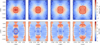 |
Fig. C.1 From left to right: 1, 2, 5, and 7 yr after the SN explosion. Note that the SN shock becomes isothermal soon before colliding with the CSM shell thus allowing the survival of a large fraction of the dust introduced by the eruption. |
It is also worth exploring the case in which the bipolar shape results from the interaction of a spherical eruption with a non- spherically symmetric stellar wind. Thus, we adopt the stellar wind model by Frank et al. (1995). Indeed, the density and velocity of the stellar wind are given by
 (C.1)
(C.1)
 (C.2)
(C.2)
where F (ϕ) is the function defined in Eq. (7).
Following Frank et al. (1995), model B12−wind considers a stellar wind consisting of a low-density component with α = 0.995, β = 2.3, Ṁw = 10−3 M⊙ yr−1, υr,0 = 250 km s−1, inserted within a radius of r0 = 0.006 pc. The wind expands into a low density uniform ambient medium with density ρamb ~ 10−27 g cm−3. This component evolves during 290 years until filling most of the computational box of (0.05 pc)3. Then, a second, denser, component is introduced for 20 years by increasing the mass input rate to Ṁw = 10−1 M⊙ yr−1 and the velocity to υr,0 = 750 km s−1. Later, a spherically symmetric stellar eruption is injected as described in Sect. 2.2 with α = 0. Finally, in order to compare this calculation with our model B12−10 (see Sect. 3.2), a SN explodes 12 yr after the eruption with the same SN parameters as in B12−10.
Figure C.1 presents the simulation results, with panels from left to right showing snapshots at t ~ 1,2,5 and 7 yr after the SN. First, note that a bipolar shape can indeed be the outcome of the interaction of a spherical eruption with the non-spherical wind. This occurs because the CSM formed by the stellar wind is significantly denser in the equatorial region, inhibiting the expansion of the eruption remnant in this direction and resulting in the bipolar morphology. The shape and size of the CSM shell prior to the SN are similar with those discussed in Sect. 3.2, thus showing that our model set-up (see Sect. 2.2) is able to describe the interaction of the eruption with the prior wind. This is even more relevant considering that here our aim is to study the outcome of the dust introduced by the eruption once the SN occurs.
Figure C.1 shows that the SN forward shock reaches large temperatures at the earliest stages of evolution (~ 107 K, see the first bottom panel in Fig. C.1). However, the shock soon becomes isothermal due to strong cooling and adopts the bipolar shape before colliding with the outer shell (middle panels in Fig. C.1), where most of the dust is located. Hence, similar to our B12−10 case, most of the dust (~ 55%, see Fig. 8) survives even after the SN shock has overrun the CSM shell, which occurs at tsn ~ 7 yr, as shown in the right columns of Fig. C.1.
Appendix D The role of radioactive heating
The total energy released by the radioactive decay chain 56Ni → 56Co → 56Fe can be approximated as (Matsumoto et al. 2025)
 (D.1)
(D.1)
For a typical value of MNi ~ 0.032 M⊙ of 56Ni produced in type II SNe (Anderson 2019), this yields approximately 5.76 × 1048 erg. This energy, assumed to be evenly distributed and instantaneously transferred to heat a 10-M⊙ ejecta (case B 12−56Ni), translates into a temperature ~ 2 × 10⁶ K. For the assumed values in cases B12−15 and B12−20, the ejecta gas temperatures are ~ 4 × 10⁷ K and ~ 8 × 10⁷ K, respectively.
Appendix E 1D density profiles
Figures E.1 and E.2 show the density profiles in the x (left) and z (right) axes at the same post-SN times shown in Figs. 4 and 6 for the B200 and B12−10 cases, respectively. It is important to note that the stellar wind, the CSM shell created by the eruption, and the SN are all in agreement with the expected in our numerical set-up (Sect. 2). Larger fluctuations in density are observed in the z-axis, which is due to the larger gas velocities in this direction.
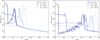 |
Fig. E.1 Density profiles along the x (left panel) and z (right panel) axes for B200. The different curves correspond to the times presented in Fig. 4. |
References
- Anderson, J. P. 2019, A&A, 628, A7 [NASA ADS] [CrossRef] [EDP Sciences] [Google Scholar]
- Andrews, J. E., & Smith, N. 2018, MNRAS, 477, 74 [Google Scholar]
- Andrews, J. E., Gallagher, J. S., Clayton, G. C., et al. 2010, ApJ, 715, 541 [Google Scholar]
- Bersten, M. C., Orellana, M., Folatelli, G., et al. 2024, A&A, 681, L18 [NASA ADS] [CrossRef] [EDP Sciences] [Google Scholar]
- Blondin, J. M., Lundqvist, P., & Chevalier, R. A. 1995, AAS Meeting Abstracts, 187, 78.01 [Google Scholar]
- Brethauer, D., Margutti, R., Milisavljevic, D., et al. 2022, ApJ, 939, 105 [Google Scholar]
- Cherchneff, I. 2013, EAS Pub. Ser., 60, 175 [Google Scholar]
- Chevalier, R. A. 1982, ApJ, 258, 790 [NASA ADS] [CrossRef] [Google Scholar]
- Chevalier, R. A., & Clegg, A. W. 1985, Nature, 317, 44 [Google Scholar]
- Chevalier, R. A., & Fransson, C. 2017, in Handbook of Supernovae, eds. A. W. Alsabti, & P. Murdin (Berlin: Springer), 875 [CrossRef] [Google Scholar]
- Chugai, N. N., & Utrobin, V. P. 2022, Astron. Lett., 48, 275 [NASA ADS] [CrossRef] [Google Scholar]
- Colella, P., & Woodward, P. R. 1984, J. Comput. Phys., 54, 174 [NASA ADS] [CrossRef] [Google Scholar]
- Crowther, P. A. 2003, Ap&SS, 285, 677 [NASA ADS] [CrossRef] [Google Scholar]
- Dalgarno, A., & McCray, R. A. 1972, ARA&A, 10, 375 [Google Scholar]
- Davidson, K. 2020, Galaxies, 8, 10 [NASA ADS] [CrossRef] [Google Scholar]
- Davidson, K., & Humphreys, R. M. 1997, ARA&A, 35, 1 [NASA ADS] [CrossRef] [Google Scholar]
- Dessart, L., Hillier, D. J., Audit, E., Livne, E., & Waldman, R. 2016, MNRAS, 458, 2094 [Google Scholar]
- Draine, B. T. 2003a, ARA&A, 41, 241 [NASA ADS] [CrossRef] [Google Scholar]
- Draine, B. T. 2003b, ApJ, 598, 1017 [NASA ADS] [CrossRef] [Google Scholar]
- Draine, B. T. 2011, Physics of the Interstellar and Intergalactic Medium (Princeton: Princeton University Press) [Google Scholar]
- Dunne, L., Maddox, S. J., Ivison, R. J., et al. 2009, MNRAS, 394, 1307 [NASA ADS] [CrossRef] [Google Scholar]
- Dwek, E. 1987, ApJ, 322, 812 [NASA ADS] [CrossRef] [Google Scholar]
- Dwek, E. 2005, AIP Conf. Ser., 804, 197 [Google Scholar]
- Dwek, E., & Werner, M. W. 1981, ApJ, 248, 138 [NASA ADS] [CrossRef] [Google Scholar]
- Dwek, E., Sarangi, A., Arendt, R. G., et al. 2021, ApJ, 917, 84 [NASA ADS] [CrossRef] [Google Scholar]
- Dyson, J. E. 1989, IAU Colloq., 350, 137 [Google Scholar]
- Elmegreen, B. G. 1981, ApJ, 251, 820 [Google Scholar]
- Frank, A., Balick, B., & Davidson, K. 1995, ApJL, 441, L77 [Google Scholar]
- Fryxell, B., Olson, K., Ricker, P., et al. 2000, ApJ, 131, 273 [Google Scholar]
- Gal-Yam, A., Leonard, D. C., Fox, D. B., et al. 2007, ApJ, 656, 372 [NASA ADS] [CrossRef] [Google Scholar]
- Gall, C., & Hjorth, J. 2018, ApJ, 868, 62 [CrossRef] [Google Scholar]
- Garcia-Segura, G., Langer, N., & Mac Low, M. M. 1996a, A&A, 316, 133 [NASA ADS] [Google Scholar]
- Garcia-Segura, G., Mac Low, M. M., & Langer, N. 1996b, A&A, 305, 229 [NASA ADS] [Google Scholar]
- Gomez, H. L., Vlahakis, C., Stretch, C. M., et al. 2010, MNRAS, 401, L48 [NASA ADS] [CrossRef] [Google Scholar]
- González, R. F., de Gouveia Dal Pino, E. M., Raga, A. C., & Velazquez, P. F. 2004, ApJL, 600, L59 [Google Scholar]
- González, R. F., Zapata, L. A., Raga, A. C., et al. 2022, A&A, 659, A168 [NASA ADS] [CrossRef] [EDP Sciences] [Google Scholar]
- Harris, C. R., Millman, K. J., van der Walt, S. J., et al. 2020, Nature, 585, 357 [NASA ADS] [CrossRef] [Google Scholar]
- Hiramatsu, D., Howell, D. A., Moriya, T. J., et al. 2021a, ApJ, 913, 55 [CrossRef] [Google Scholar]
- Hiramatsu, D., Howell, D. A., Van Dyk, S. D., et al. 2021b, Nat. Astron., 5, 903 [NASA ADS] [CrossRef] [Google Scholar]
- Humphreys, R., & Davidson, K. 1994, PASP, 106, 1025 [NASA ADS] [CrossRef] [Google Scholar]
- Humphreys, R. M., & Martin, J. C. 2012, Astrophys. Space Sci. Lib., 384, 1 [Google Scholar]
- Hunter, J. D. 2007, Comput. Sci. Eng., 9, 90 [NASA ADS] [CrossRef] [Google Scholar]
- Jiménez, S., Tenorio-Tagle, G., & Silich, S. 2021, MNRAS, 505, 4669 [Google Scholar]
- Kirchschlager, F., Schmidt, F. D., Barlow, M. J., et al. 2019, MNRAS, 489, 4465 [CrossRef] [Google Scholar]
- Kirchschlager, F., Barlow, M. J., & Schmidt, F. D. 2020, ApJ, 893, 70 [CrossRef] [Google Scholar]
- Kochanek, C. S. 2011, ApJ, 743, 73 [NASA ADS] [CrossRef] [Google Scholar]
- Kumar, B., Eswaraiah, C., Singh, A., et al. 2019, MNRAS, 488, 3089 [NASA ADS] [CrossRef] [Google Scholar]
- Mac Low, M.-M., & McCray, R. 1988, ApJ, 324, 776 [NASA ADS] [CrossRef] [Google Scholar]
- Mac Low, M. M., Langer, N., & García-Segura, G. 1996, BAAS, 28, 882 [Google Scholar]
- MacNeice, P., Spicer, D. S., & Antiochos, S. K. 1999, ESA SP, 448, 459 [Google Scholar]
- Madura, T. I., Gull, T. R., Owocki, S. P., et al. 2012, MNRAS, 420, 2064 [NASA ADS] [CrossRef] [Google Scholar]
- Margalit, B. 2022, ApJ, 933, 238 [Google Scholar]
- Martínez-González, S., Wünsch, R., Palouš, J., et al. 2018, ApJ, 866, 40 [Google Scholar]
- Martínez-González, S., Wünsch, R., Silich, S., et al. 2019, ApJ, 887, 198 [CrossRef] [Google Scholar]
- Martínez-González, S., Silich, S., & Tenorio-Tagle, G. 2021, MNRAS, 507, 1175 [Google Scholar]
- Martínez-González, S., Wünsch, R., Tenorio-Tagle, G., et al. 2022, ApJ, 934, 51 [Google Scholar]
- Martinez, L., Bersten, M. C., Folatelli, G., Orellana, M., & Ertini, K. 2024, A&A, 683, A154 [NASA ADS] [CrossRef] [EDP Sciences] [Google Scholar]
- Massey, P., Plez, B., Levesque, E. M., et al. 2005, ApJ, 634, 1286 [NASA ADS] [CrossRef] [Google Scholar]
- Matsumoto, T., Metzger, B. D., & Goldberg, J. A. 2025, ApJ, 978, 56 [Google Scholar]
- Matsuura, M., Barlow, M. J., Zijlstra, A. A., et al. 2009, MNRAS, 396, 918 [NASA ADS] [CrossRef] [Google Scholar]
- Mauerhan, J. C., Van Dyk, S. D., Johansson, J., et al. 2017, ApJ, 834, 118 [Google Scholar]
- Mauerhan, J. C., Filippenko, A. V., Zheng, W., et al. 2018, MNRAS, 478, 5050 [NASA ADS] [CrossRef] [Google Scholar]
- Micelotta, E. R., Matsuura, M., & Sarangi, A. 2018, Space Sci. Rev., 214, 53 [NASA ADS] [CrossRef] [Google Scholar]
- Moriya, T. J., Blinnikov, S. I., Tominaga, N., et al. 2013, MNRAS, 428, 1020 [NASA ADS] [CrossRef] [Google Scholar]
- Nozawa, T., Kozasa, T., Tominaga, N., et al. 2010, ApJ, 713, 356 [NASA ADS] [CrossRef] [Google Scholar]
- Ono, M., Nozawa, T., Nagataki, S., et al. 2024, ApJ, 271, 33 [Google Scholar]
- Oskinova, L. M., Hamann, W. R., & Feldmeier, A. 2007, A&A, 476, 1331 [NASA ADS] [CrossRef] [EDP Sciences] [Google Scholar]
- Ostriker, J., & Silk, J. 1973, ApJL, 184, L113 [Google Scholar]
- Pan, T., Patnaude, D., & Loeb, A. 2013, MNRAS, 433, 838 [CrossRef] [Google Scholar]
- Pearson, J., Hosseinzadeh, G., Sand, D. J., et al. 2023, ApJ, 945, 107 [NASA ADS] [CrossRef] [Google Scholar]
- Pittard, J. M. 2013, MNRAS, 435, 3600 [NASA ADS] [CrossRef] [Google Scholar]
- Priestley, F. D., Chawner, H., Matsuura, M., et al. 2021, MNRAS, 500, 2543 [Google Scholar]
- Priestley, F. D., Arias, M., Barlow, M. J., & De Looze, I. 2022, MNRAS, 509, 3163 [Google Scholar]
- Qin, Y.-J., Zhang, K., Bloom, J., et al. 2024, MNRAS, 534, 271 [NASA ADS] [CrossRef] [Google Scholar]
- Rodríguez, Ó., Meza, N., Pineda-García, J., & Ramirez, M. 2021, MNRAS, 505, 1742 [CrossRef] [Google Scholar]
- Sarangi, A., & Slavin, J. D. 2022, ApJ, 933, 89 [NASA ADS] [CrossRef] [Google Scholar]
- Sarangi, A., Matsuura, M., & Micelotta, E. R. 2018, Space Sci. Rev., 214, 63 [NASA ADS] [CrossRef] [Google Scholar]
- Schure, K. M., Kosenko, D., Kaastra, J. S., Keppens, R., & Vink, J. 2009, A&A, 508, 751 [NASA ADS] [CrossRef] [EDP Sciences] [Google Scholar]
- Silich, S., Tenorio-Tagle, G., & Muñoz-Tuñón, C. 2003, ApJ, 590, 791 [NASA ADS] [CrossRef] [Google Scholar]
- Smith, N. 2006, ApJ, 644, 1151 [Google Scholar]
- Smith, N. 2010, MNRAS, 402, 145 [NASA ADS] [CrossRef] [Google Scholar]
- Smith, N. 2011, Bulletin de la Societe Royale des Sciences de Liege, 80, 322 [Google Scholar]
- Smith, N. 2014, ARA&A, 52, 487 [NASA ADS] [CrossRef] [Google Scholar]
- Smith, N. 2017, in Handbook of Supernovae, eds. A. W. Alsabti, & P. Murdin (Berlin: Springer), 403 [Google Scholar]
- Smith, N., & Andrews, J. E. 2020, MNRAS, 499, 3544 [NASA ADS] [CrossRef] [Google Scholar]
- Smith, N., & Ferland, G. J. 2007, ApJ, 655, 911 [NASA ADS] [CrossRef] [Google Scholar]
- Smith, R. K., & Hughes, J. P. 2010, ApJ, 718, 583 [NASA ADS] [CrossRef] [Google Scholar]
- Smith, N., Chornock, R., Silverman, J. M., Filippenko, A. V., & Foley, R. J. 2010, ApJ, 709, 856 [NASA ADS] [CrossRef] [Google Scholar]
- Smith, B. D., Bryan, G. L., Glover, S. C. O., et al. 2017, MNRAS, 466, 2217 [NASA ADS] [CrossRef] [Google Scholar]
- Smith, N., Andrews, J. E., Rest, A., et al. 2018, MNRAS, 480, 1466 [Google Scholar]
- Smith, N., Andrews, J. E., Milne, P., et al. 2024, MNRAS, 530, 405 [NASA ADS] [CrossRef] [Google Scholar]
- Spitzer, L. 1962, Physics of Fully Ionized Gases (Geneva: Interscience Publishers) [Google Scholar]
- Steffen, W., Teodoro, M., Madura, T. I., et al. 2014, MNRAS, 442, 3316 [CrossRef] [Google Scholar]
- Szalai, T., Fox, O. D., Arendt, R. G., et al. 2021, ApJ, 919, 17 [NASA ADS] [CrossRef] [Google Scholar]
- Szécsi, D., Agrawal, P., Wünsch, R., & Langer, N. 2022, A&A, 658, A125 [NASA ADS] [CrossRef] [EDP Sciences] [Google Scholar]
- Taddia, F., Stritzinger, M. D., Sollerman, J., et al. 2013, A&A, 555, A10 [NASA ADS] [CrossRef] [EDP Sciences] [Google Scholar]
- Tang, X., & Chevalier, R. A. 2017, MNRAS, 465, 3793 [CrossRef] [Google Scholar]
- Tartaglia, L., Pastorello, A., Sollerman, J., et al. 2020, A&A, 635, A39 [NASA ADS] [CrossRef] [EDP Sciences] [Google Scholar]
- Temim, T., Dwek, E., Tchernyshyov, K., et al. 2015, ApJ, 799, 158 [NASA ADS] [CrossRef] [Google Scholar]
- Tenorio-Tagle, G., Bodenheimer, P., Franco, J., & Rozyczka, M. 1990, MNRAS, 244, 563 [NASA ADS] [Google Scholar]
- Tenorio-Tagle, G., Silich, S., Martínez-González, S., Terlevich, R., & Terlevich, E. 2015, ApJ, 800, 131 [Google Scholar]
- Tielens, A. G. G. M. 2005, The Physics and Chemistry of the Interstellar Medium (Cambridge: Cambridge University Press) [Google Scholar]
- Todini, P., & Ferrara, A. 2001, MNRAS, 325, 726 [NASA ADS] [CrossRef] [Google Scholar]
- Truelove, J. K., & McKee, C. F. 1999, ApJ, 120, 299 [Google Scholar]
- Trundle, C., Kotak, R., Vink, J. S., & Meikle, W. P. S. 2008, A&A, 483, L47 [NASA ADS] [CrossRef] [EDP Sciences] [Google Scholar]
- van Marle, A. J., Langer, N., & García-Segura, G. 2004, in Revista Mexicana de Astronomia y Astrofisica Conference Ser., 22, 136 [Google Scholar]
- van Marle, A. J., Smith, N., Owocki, S. P., & van Veelen, B. 2010, MNRAS, 407, 2305 [Google Scholar]
- Virtanen, P., Gommers, R., Oliphant, T. E., et al. 2020, Nat. Methods, 17, 261 [Google Scholar]
- Vlasis, A., Dessart, L., & Audit, E. 2016, MNRAS, 458, 1253 [Google Scholar]
- Wang, L.-J., Liu, L.-D., Lin, W.-L., et al. 2022, ApJ, 933, 102 [CrossRef] [Google Scholar]
- Weaver, R., McCray, R., Castor, J., Shapiro, P., & Moore, R. 1977, ApJ, 218, 377 [Google Scholar]
- Weis, K. 2012, in Astrophysics and Space Science Library, Eta Carinae and the Supernova Impostors, ed. K. Davidson & R. M. Humphreys, 384, 171 [NASA ADS] [Google Scholar]
- Wong, K.-W., Irwin, J. A., Wik, D. R., et al. 2016, ApJ, 829, 49 [NASA ADS] [CrossRef] [Google Scholar]
- Woosley, S. E., Blinnikov, S., & Heger, A. 2007, Nature, 450, 390 [NASA ADS] [CrossRef] [PubMed] [Google Scholar]
- Wünsch, R., Tenorio-Tagle, G., Palouš, J., & Silich, S. 2008, ApJ, 683, 683 [Google Scholar]
- Wünsch, R., Palouš, J., Tenorio-Tagle, G., & Ehlerová, S. 2017, ApJ, 835, 60 [CrossRef] [Google Scholar]
At a fixed cell size, refinement level 5 corresponds to an equivalent uniform grid of (128)3 cells, and refinement level 7 corresponds to (512)3 cells. Similarly, at refinement level 6, there are (256)3 cells on the equivalent uniform grid, and at refinement level 8, there are (1024)3 cells.
All Tables
All Figures
|
Fig. 1 Schematic (not to scale) of a SNR evolving within a bipolar CSM created by a stellar eruption, subsequent to the ejection of the stellar wind. Panel a shows the expansion of the SN ejecta and the forward shock at early times after the explosion. Panel b presents the time when the SN begins to interact with the densest medium left by the eruption. |
| In the text | |
|
Fig. 2 Normalized density distributions of ejected material during the eruption and the SN ejecta expressed as a function of we = r/Re and wsn = r/Rsn, respectively. Note that the CSM follows a shell-like density structure. |
| In the text | |
|
Fig. 3 Evolution of the SNR within the erupted CSM for S 200, with each column showing snapshots at tSN = 4,40,170, and 250 yr after the SN explosion, respectively. From top to bottom, each row displays, in log scale, the number gas density, the gas temperature, and the dust mass density. |
| In the text | |
|
Fig. 4 Same as Fig. 3 but for B200, with snapshots at tSN = 4,20,75, and 115 yr, respectively. Additional 1D density profiles along the x and z axes are provided in Appendix E. |
| In the text | |
|
Fig. 5 Upper panels: SNR (only gas) kinetic (solid), thermal (dotted), and radiated (dashed) energies as a function of time for S200 (left) and B200 (right). Lower panels: evolution of the dust mass, normalized to that ejected by the eruption. For all panels, thicker lines correspond to S200 and S200, while thinner lines to B200−Test and S200−Test, respectively. |
| In the text | |
|
Fig. 6 Same as Fig. 4 but for B 12−10, with snapshots at tSN = 0.1,1,7 , and 10 yr after the SN explosion, respectively. Note in the last column that several blisters of shock-heated gas already extend beyond the CSM density distribution. Additional 1D density profiles along the x and z axes are provided in Appendix E. |
| In the text | |
|
Fig. 7 Gas temperature distribution slices in the x−z plane, with the first row showing results for B12−15 and the second row for B12−20. |
| In the text | |
|
Fig. 8 Same as Fig. 5 but for B12−10,B12−56Ni, B12−15, B12−20, and B12−wind (see Appendix C). Note that while the curves corresponding to cases B12−10 and B12−56Ni are presented up to 10 years post-SN, the ones corresponding to B12−15, B12−20, and B12−wind are presented only up to 7–8 years, as the simulations have reached the boundaries of the computational domain, but the most relevant phase of their evolution has already taken place. |
| In the text | |
|
Fig. C.1 From left to right: 1, 2, 5, and 7 yr after the SN explosion. Note that the SN shock becomes isothermal soon before colliding with the CSM shell thus allowing the survival of a large fraction of the dust introduced by the eruption. |
| In the text | |
|
Fig. E.1 Density profiles along the x (left panel) and z (right panel) axes for B200. The different curves correspond to the times presented in Fig. 4. |
| In the text | |
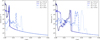 |
Fig. E.2 Same as Fig. E.1 but for B12−10. |
| In the text | |
Current usage metrics show cumulative count of Article Views (full-text article views including HTML views, PDF and ePub downloads, according to the available data) and Abstracts Views on Vision4Press platform.
Data correspond to usage on the plateform after 2015. The current usage metrics is available 48-96 hours after online publication and is updated daily on week days.
Initial download of the metrics may take a while.