| Issue |
A&A
Volume 691, November 2024
|
|
|---|---|---|
| Article Number | A42 | |
| Number of page(s) | 22 | |
| Section | Stellar structure and evolution | |
| DOI | https://doi.org/10.1051/0004-6361/202449575 | |
| Published online | 01 November 2024 | |
The red giant branch tip in the SDSS, PS1, JWST, NGRST, and Euclid photometric systems
Calibration in optical passbands using Gaia DR3 synthetic photometry
INAF – Osservatorio di Astrofisica e Scienza dello Spazio di Bologna, via Piero Gobetti 93/3, 40129 Bologna, Italy
⋆ Corresponding author; michele.bellazzini@inaf.it
Received:
12
February
2024
Accepted:
7
August
2024
We used synthetic photometry from Gaia DR3 BP and RP spectra for a large selected sample of stars in the Large Magellanic Cloud (LMC) and Small Magellanic Cloud (SMC) to derive the magnitude of the red giant branch (RGB) tip for these two galaxies in several passbands across a range of widely used optical photometric systems, including those of space missions that have not yet started their operations. The RGB tip is estimated by fitting a well motivated model to the RGB luminosity function (LF) within a fully Bayesian framework, allowing for a proper representation of the uncertainties of all the involved parameters and their correlations. By adopting the best available distance and interstellar extinction estimates, we provide a calibration of the RGB tip as a standard candle for the following passbands: Johnson-Kron-Cousins I (mainly used for validation purposes), Hubble Space Telescope F814W, Sloan Digital Sky Survey i and z, PanSTARRS 1 y, James Webb Space Telescope F090W, Nancy Grace Roman Space Telescope Z087, and Euclid IE, with an accuracy within a few per cent, depending on the case. We used theoretical models to explore the trend of the absolute magnitude of the tip as a function of colour in the different passbands (beyond the range spanned by the LMC and SMC), as well as its dependency on age. These calibrations can be very helpful to obtain state-of-the-art RGB tip distance estimates to stellar systems in a very large range of distances directly from data in the natural photometric system of these surveys and/or missions, without recurring to photometric transformations. We have made the photometric catalogues publicly available for calibrations in additional passbands or for different approaches in the estimate of the tip, as well as for stellar populations and stellar astrophysics studies that may take advantage of large and homogeneous datasets of stars with magnitudes in 22 different passbands.
Key words: techniques: photometric / catalogs / stars: distances / Magellanic Clouds / distance scale
© The Authors 2024
 Open Access article, published by EDP Sciences, under the terms of the Creative Commons Attribution License (https://creativecommons.org/licenses/by/4.0), which permits unrestricted use, distribution, and reproduction in any medium, provided the original work is properly cited.
This article is published in open access under the Subscribe to Open model. Subscribe to A&A to support open access publication.
1. Introduction
The tip of the red giant branch (RGB) is a well known and well understood feature of the colour-magnitude diagrams (CMDs) of stellar systems hosting significant populations of stars older than ≃2 Gyr (see e.g. Salaris & Cassisi 1998; Barker et al. 2004; Bellazzini 2008; Serenelli et al. 2017; Madore & Freedman 2020; Li et al. 2023, and references therein). For stars in the mass range ≃0.5 − 2.0 M⊙ the luminosity of RGB stars mainly depends on the mass of the degenerate He core (Mc), which is nearly constant at the violent onset of the core He-burning phase (He flash, Serenelli et al. 2017). The sudden change in the evolutionary phase from shell H-burning (RGB) to core He-burning (red clump, RC, for the intermediate-age stars, and horizontal branch, HB, for the oldest stars) induces a strong discontinuity at the bright end of the RGB LF; this is the specific observable we refer when using the term ‘RGB tip’ (Lee et al. 1993; Madore & Freedman 1995). The constancy of Mc values at the tip and, consequently, the near-constancy of the luminosity of the feature provide the key characteristics for a standard candle in this context. In particular, the magnitude of the RGB tip in the reddest optical passbands, typically the Johnson-Kron-Cousins I band, has been shown to be very mildly dependent on metallicity (as well as on other stellar parameters) and nearly constant for [Fe/H] ≤ −0.7 (Da Costa & Armandroff 1990; Barker et al. 2004; Bellazzini 2008; Serenelli et al. 2017); whereas, it is linearly correlated with metallicity in the near infrared passbands (see e.g. Bellazzini et al. 2004a; Valenti et al. 2004; Serenelli et al. 2017, and references therein).
Introduced in its modern form in the early 1990s (Lee et al. 1993; Madore & Freedman 1995; Sakai et al. 1996) the use of the RGB tip as a standard candle has become a precious and widely adopted tool in the establishment of the local and cosmological distance scales (see e.g. Maíz-Apellániz et al. 2002; Bellazzini et al. 2004b, 2005; Conn et al. 2012, 2016; Freedman et al. 2019; Anand et al. 2021; Scolnic et al. 2023; Madore et al. 2023 and references therein). The behaviour of the observable and of the associated biases and uncertainties have also been studied extensively (Madore & Freedman 1995; Salaris & Cassisi 1998; Bellazzini et al. 2002; Barker et al. 2004; Serenelli et al. 2017; Madore & Freedman 2020; Saltas & Tognelli 2022; Madore et al. 2023; Wu et al. 2023; Anderson et al. 2024).
While classical calibrations of the RGB tip have been based on the RR Lyrae / HB distance scale (see e.g. Lee et al. 1993; Rizzi et al. 2007) or on theoretical models (Salaris & Cassisi 1998), Bellazzini et al. (2001) introduced a new calibration whose zero point was anchored to the semi-geometrical distance to the massive globular cluster ω Centauri, obtained by Thompson et al. (2001) from a double-lined detached eclipsing binary within the cluster, OGLE 17. Two decades later, accurate distance estimates from eclipsing binaries have become available for two local galaxies that stand as classical pillars of the cosmological distance scale, namely: the Large Magellanic Cloud (LMC; Pietrzyński et al. 2019) and the Small Magellanic Cloud (SMC; Graczyk et al. 2020). Hoyt (2023, H23 hereafter) took advantage of these new distance measurements, as well as the large sample of LMC and SMC photometry provided by the Optical Gravitational Lensing Experiment (OGLE) project (Udalski et al. 2008a,b) and new reddening maps from the same project (Skowron et al. 2021) to derive, through a careful and insightful analysis, a new calibration of the RGB tip in the I band. This calibration was aimed at ensuring ≃1% consistency in terms of distance (see Soltis et al. 2021; Li et al. 2022, 2023; Dixon et al. 2023 for recent attempts of direct calibration of the standard candle using astrometry from the ESA-Gaia mission Gaia Collaboration 2016, 2021a).
In the present contribution, we follow the path traced by H23, but using large samples of LMC and SMC stars with synthetic photometry from the Gaia-DR3 (Gaia Collaboration 2023b) externally calibrated BP and RP (XP, hereafter) spectra (De Angeli et al. 2023; Montegriffo et al. 2023). As illustrated in detail in Gaia Collaboration (2023a), especially for the red passbands that are the most suitable for a safe use of the RGB tip as a standard candle, synthetic photometry that is accurate to 2–3% over a large range of colours (spectral types) can be obtained from XP spectra for any wide passband enclosed in their spectral range. Moreover, Gaia Collaboration (2023a) used selected samples of photometric standard stars to enhance the accuracy of the XP synthetic photometry (XPSP) in a few widely used photometric systems, in a process they refer to as ‘standardisation’. In these cases, a photometric accuracy at a level of a few millimag has been achieved.
As suggested by Bellazzini (2008) and demonstrated by means of theoretical models in a number of studies, other passbands sampling the stellar spectrum in the range 700 nm ≲ λ ≲ 1100 nm may be effective in tracing the RGB tip with minimal dependency on metallicity and age, as for IJKC. Taking advantage of the broad flexibility enabled by XP synthetic photometry, we can directly estimate the magnitude of the RGB tip in several suitable passbands in different photometric systems. Thus, we are able to extend the calibration of the RGB tip as a standard candle beyond the JKC system to other widely used systems as those of the Sloan Digital Sky Survey (SDSS Fukugita et al. 1996) or Pan-STARRS 1 (PS1 Magnier et al. 2020), as well as those of space missions that have recently started operations, including James Webb Space Telescope (JWST1) and Euclid2, or those that are yet to be launched, such as Nancy Grace Roman Space Telescope (NGSRT3). In this way, we can provide access to the tools necessary to derive distance estimates from observations of the RGB of stellar systems over a very wide range of distances directly from the observations performed in the photometric systems of these surveys and space missions, without recurring to uncertain and possibly biased photometric transformations (see Gaia Collaboration 2023a for discussion and references, and Anderson et al. 2024 for a recent application to the same problem).
The plan of the paper is as follows. In Sect. 2, we present the samples of SMC and LMC stars that we used to estimate the magnitude of the tip in different passbands and how we correct observed synthetic magnitudes of these stars for interstellar extinction. In Sect. 3, we describe the results of our measurements of the RGB tip and we provide the calibrations of the absolute magnitude of the tip in different passbands as a function of colour, extending the colour range of applicability with the help of theoretical models. In Sect. 5 we introduce the bayesian method that we use to measure the tip, briefly discussing its robustness, quality, and limitations. Finally, we summarise our results and draw our conclusions in Sect. 6.
In Appendix A, we display the diagrams of the actual detection of the tip in the various considered passbands. In Appendix B, we discuss the possible reasons for the ≃0.05 mag difference in our estimates of the RGB tip of the LMC and SMC, with respect to those obtained by H23, while in Appendix D we briefly describe the LMC and SMC catalogues with XPSP in 22 passbands that we used in the present study and that we make publicly available. Finally, in Appendix E, we report on the parameters obtained from the RGB tip fitting procedure, their uncertainties, and give further details on the tests we performed.
2. Samples
As a first step, we consider here only stars that are included in the Gaia Synthetic Photometry Catalogue (GSPC; Gaia Collaboration 2023a)4 to avoid stars with low photometric signal-to-noise ratio (S/N) in any of the GSPC passbands. Then, to remove sources with possibly flawed astrometry, we considered only those stars with RUWE < 1.3 (Lindegren et al. 2021). To minimise the effects of blendings and contamination in the photometry of individual stars we also require |C⋆|< σC⋆(G), according to Eq. 18 of Riello et al. (2021).
Hence, we selected from the GSPC stars satisfying the above quality criteria and lying (a) within 10 degrees from the centre of the LMC and within 2.0 mas/yr from its mean proper motion (LMC sample) and (b) within 8 degrees from the centre of the SMC and within 1.5 mas/yr from its mean proper motion (SMC sample), where the galaxy centres and mean proper motions at the centre have been taken from Gaia Collaboration (2021b). Finally, removing all stars having error on the parallax lower than 20% (18 242 and 3752 for the LMC and SMC samples, respectively) was a simple and very efficient mean to select out foreground Galactic stars. The resulting LMC sample contains 603 311 stars, while the SMC sample contains 124 578 stars5.
For each of these stars a value of the interstellar reddening E(B − V) was derived from the maps by Skowron et al. (2021), when available, and from the maps by Schlegel et al. (1998), re-calibrated by Schlafly & Finkbeiner (2011) in regions not reached by the former map. Skowron et al. (2021) reddening values are in the same scale as Schlafly & Finkbeiner (2011); this has been verified for the stars in common in the outer regions of the galaxies where the comparison is meaningful (Schlegel et al. 1998). To convert E(V − I) provided by Skowron et al. (2021) into E(B − V) we used the equation E(B − V) = E(V − I)/1.399, from Schlafly & Finkbeiner (2011, their Table 6, see below).
In selecting the stars to be used for a clean detection of the RGB tip in the LMC and SMC H23 excluded from the sample the regions of the OGLE-III photometric maps where recent or ongoing star formation can inject into the colour-magnitude diagram (CMD) young core He-burning stars that can contaminate the RGB, making the detection of the tip more uncertain (see Appendix B for further details and discussion). Following this approach, we adopt a simple selection in angular distance from the galaxy centre (see below) and in interstellar extinction, taking advantage of the fact that the young stellar populations are concentrated in the central regions of both galaxies and that they are typically associated with higher concentrations of dust, hence, high extinction.
For both galaxies, our starting sample is much more extended in area than the OGLE-III footprint and contains a much larger number of bright stars. For example, for LMC our original sample contains approximately two times the stars in the OGLE-III sample for G < 17.65 (the magnitude limit of GSPC Gaia Collaboration 2023a). Hence, we were allowed to be more conservative than H23 in keeping only the less extincted and less contaminated by young populations outer regions of the galaxies. In particular, we adopted the following selection criteria:
-
LMC: we retain only 202259 stars having E(B − V) < 0.2 and with an angular distance larger than 3.8° from (RA, Dec) = (81.28 ° , − 69.00 ° ),
-
SMC: we retain only 43152 stars having E(B − V) < 0.2 and Rang > 1.8° from (RA, DEC) = (15.00 ° , − 72.70 ° ).
In both cases, the radial selection was not performed with respect to the centre of the galaxies (as provided, e.g. by Gaia Collaboration 2021b), but with respect to an off-set position optimising the removal of star-forming regions from the sample with a simple circular cut. We did not attempt to correct for the 3D structure of the two galaxies, which is known to have non-negligible effects in both cases (see e.g. Choi et al. 2018; Gaia Collaboration 2021b; Zivick et al. 2021; Omkumar et al. 2021; Tatton et al. 2021; Cullinane et al. 2023; Murray et al. 2024). Our approach is to average out these effects by means of large samples, with reasonably balanced distributions in azimuth. In Appendix C, we provide evidence supporting the validity of this choice.
The results of the selection are illustrated in Fig. 1, where the finally selected samples are plotted in the Viridis density scale. For both galaxies ample fractions of the regions selected by H23 for his calibration are included in our samples. For the SMC, we decided to keep in the sample stars in the Magellanic Bridge (see Gaia Collaboration 2021b, for references) as we verified that the actual contamination of the RGB by young stars from this relatively small low-surface-density region is negligible.
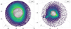 |
Fig. 1. Distribution in the sky of the stars in our LMC sample (left panel) and SMC sample (right panel). Stars are colour-coded according to the local surface density. Stars excluded from the sample used for the detection of the RGB tip are plotted in grey-scale, while those retained are plotted in Viridis scale. |
Drawing from the GSPC, we obtained for all the selected stars ‘standardised’ magnitudes, fluxes, and uncertainties on the fluxes in the following passbands: JKC UBVRI, SDSS ugriz, Hubble Space Telescope (HST) ACS-WFC6 F606W and F814W. Then we used GaiaXPy7 (De Angeli et al. 2023; Gaia Collaboration 2023a) to obtain (for the same stars) standardised magnitudes and fluxes + uncertainties in PS1 grizy8, and non-standardised magnitudes and fluxes + uncertainties in JWST-NIRCAM F070W and F090W (VEGAMAG), NGRST R062 and Z087 (VEGAMAG), and in Euclid-VIS IE (ABMAG; Cuillandre et al. 2024).
The uncertainties on magnitudes (ϵmag) have been obtained from the uncertainties on fluxes (ϵflux) as:
Each magnitude has been corrected for extinction using the reddening laws from Table 6 of Schlafly & Finkbeiner (2011) with RV = 3.1, when available. In particular, we adopted9:
For passbands not included in that table, namely those in the JWST-NIRCAM, NGRST and Euclid systems, we adopted the reddening laws computed by the interface to the Padua stellar models10 (Bressan et al. 2012) for a G2V star adopting the Cardelli et al. (1989) extinction curve for RV = 3.1, in particular:
Given the restrictive reddening constraints adopted in the selection of our sample, the uncertainties in the Aλ/E(B − V) coefficients as well as neglecting the colour dependencies of the reddening laws should have negligible effects on the final correction.
In Fig. 2, we show the CMDs of the original (greyscale) and selected (viridis) samples for both galaxies. It is clear that large sets of genuine RGB stars can be very cleanly selected in the CMD, with a very low degree of contamination from other stellar types near the RGB tip. A rich population of asymptotic giant branch (AGB) stars is present above the tip, but the discontinuity in the RGB LF is clearly evident (around G0 ≃ 15.5 and G0 ≃ 15.8 in the LMC and SMC, respectively), also in a passband showcasing a strong dependency of the RGB tip magnitude from colour, owing to the inclusion of a much bluer range of wavelength with respect to the red passbands that minimise these effects. In the following, we select our sample of RGB stars for the detection of the tip with a simple selection in the CMD, by means of a pair of parallel lines enclosing the vast majority of RGB stars within a couple of magnitudes from the tip. We verified that the adopted selections in the various CMDs are consistent with one another; hence, we are approximately using the same set of RGB stars in each passband and photometric system. For simplicity we decided to derive a single value of the RGB tip for each galaxy, associated with a mean colour, avoiding any colour splitting of the RGB of the LMC (see H23).
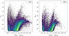 |
Fig. 2. CMD of the stars in our LMC sample (left panel) and SMC sample (right panel) in the Gaia DR3 photometric system. The meaning of symbols and colours is the same as in Fig. 1. |
To transform extinction-corrected apparent magnitudes of the tip into absolute magnitudes, we adopted the distance moduli from the measurement of the eclipsing binaries, which is (m − M)0 = 18.477 ± 0.026 for the LMC (Pietrzyński et al. 2019), and (m − M)0 = 18.997 ± 0.032 (Graczyk et al. 2020), where we summed in quadrature the statistic and systematic uncertainties quoted by these authors into a single uncertainty value. In the following, we will always use, as a reference, theoretical predictions for the magnitude of the RGB tip as a function of colour derived from PARSEC isochrones (Bressan et al. 2012), obtained from the CMD 3.7 web interface11, as it provides stellar models in all the photometric systems considered here.
There are a few additional properties of the sample, inherent to the Gaia XPSP, which are worth reporting here. In Gaia Collaboration (2023a), the photometry in the JKC and SDSS systems has been standardised against large sets of reliable and well-tested standard stars, a large collection of Landolt’s standard (Landolt 1992, 2007, 2009, 2013 and Landolt & Uomoto 2007), later critically assessed by Pancino et al. (2022) and the most-recent Stripe 82 set by Thanjavur et al. (2021), respectively. Hence, BVRI and griz XPSP magnitudes12 for these systems should be considered as the most reliably and robustly tested to reproduce the original systems with high accuracy. Magnitudes in the PS1 system (grizy) have also been standardised against a large sample of high-quality PS1 photometry but not from a ‘standard set’, just a suitable patch of the survey catalogue (Magnier et al. 2020). Magnitudes in the ACS-WFC system have been standardised against a relatively small dataset of globular cluster stars (Nardiello et al. 2018), for reasons discussed in Gaia Collaboration (2023a). The XPSP photometry reproduces magnitudes in these systems with accuracy comparable to the two cases above but the standardisation is based on (slightly for PS1, significantly for ACS-WFC) less robust external datasets.
The XPSP for the JWST-NIRCAM, NGRST, and Euclid-VIS systems is not standardised, as there were no external dataset to be used for this purpose. In this case, the accuracy can be tentatively inferred from that measured by Gaia Collaboration (2023a) in standardised systems before standardisation in passbands covering similar ranges of wavelength as those considered here for RGB tip calibration13. This is typically ≃0.01 mag, but in some cases, it reaches 0.03 − 0.04 mag: this is an intrinsic unavoidable uncertainty affecting the RGB tip calibrations derived below for magnitudes from non-standardised XPSP. In Sect. 4, we illustrate how the uncertainty in the photometric zero points can be taken into account in our final calibrations of the RGB tip. The non-standardised Gaia XPSP is also affected by a trend with magnitude, the so called ‘hockey stick’ effect, but its amplitude is negligible in the range of magnitudes where the MC tips lie, namely, < 0.01 for G ≤ 16.0.
Finally, Gaia Collaboration (2023a) showed that the photometric uncertainty associated with each individual XPSP flux is typically underestimated by a factor ranging from ≃1 up to ≃5, depending on the star’s magnitude. This effect has been corrected with an empirical formula provided in Gaia Collaboration (2023a) and included in GaiaXPy, for all the systems available in the GaiaXPy repository at that epoch. The individual photometric errors in our samples are corrected in this way for all the magnitudes except for Euclid-VIS IE14.
3. RGB tip of the LMC and SMC from XPSP: Validation and methods
In Fig. 3, the measurement of the RGB tip in the LMC and SMC in the JKC I band is given. The measurement was performed by fitting, to the RGB LF, a model similar to those published in Méndez et al. (2002), Makarov et al. (2006), Conn et al. (2011, 2012, 2016). The details of our version of this method are described in Sect. 5.2.
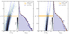 |
Fig. 3. Measuring the RGB tip in JKC I band in the LMC (left pair of panels) and in the SMC (right pair of panels). The left panels of each pair display the CMD of the considered sample with the selection of the RGB + AGB sub-sample that is later used to construct the LF (stars enclosed within the blue parallel lines). The orange horizontal line marks the position of the RGB tip and the shaded bands show the 1σ and 3σ confidence intervals. The right panels of each pair show the LF of the selected RGB + AGB sub-sample (light-blue histogram) and the best-fit model which we used to estimate ITRGB. |
The RGB tip is very cleanly detected in both galaxies at  for the LMC and at
  for the SMC, where the reported uncertainties are proxies for the 1(3)σ confidence intervals; in particular, they are the 16th (0.15th) and 84th (99.85th) percentiles of the posteriori distribution of I0TRGB (see Sect. 5.2). The colour of the RGB tip corresponding to the aforementioned measurements is estimated as the median colour of the RGB stars with a magnitude within the 1σ confidence interval of the tip magnitude. The associated uncertainty is calculated as the 16th and 84th percentiles of the colour distribution of stars with that magnitude. In all the cases presented in the following analysis, this is the method employed to evaluate the colour of the RGB tip.
As a consistency check, H23 computed the difference between the measured RGB tip of the LMC and the SMC, obtaining Δμ = 0.488 ± 0.024 (Δμ = 0.494 applying the colour correction by Jang & Lee 2017, accounting for the colour difference between the RGB tip of the two galaxies); this result is in excellent agreement with the difference between the distance moduli measured with eclipsing binaries Δμ = 0.500 ± 0.017 (Pietrzyński et al. 2019; Graczyk et al. 2020). From our measurement, we obtained Δμ = 0.494 ± 0.016 (Δμ = 0.506 applying the colour correction), which is in excellent agreement with both the H23 result and the reference value from eclipsing binaries and more closely matching the latter value than the result obtained by H23. On the other hand, our measurements of the RGB tip are fainter than those obtained by H23 by 0.061 ± 0.009 mag for the LMC (formally a full 6.8σ difference) and by 0.067 ± 0.027 mag for the SMC (2.5σ). In Appendix B, we explore the possible reasons for this discrepancy in detail.
H23 showed that many recent calibrations of the RGB tip in I band have a zero point (ZP) in the range between MITRGB ≃ −4.00 and MITRGB ≃ −4.05 (see e.g. Dixon et al. 2023, for a recent example), with a few cases in which fainter ZP are obtained (MITRGB ≃ −3.97; Yuan et al. 2019; Soltis et al. 2021; Li et al. 2023). H23 argued that the latter calibrations are based on faint measurements of the tip of the LMC due to an improper correction of the extinction and (above all) selection of the fields, with respect to his analysis (in Appendix B, we address this specific point in our case). Figure 4 shows very clearly that due to the differences in I0TRGB mentioned above, the ZP of our calibration of the RGB tip (MITRGB = −3.98 ± 0.03 for the LMC) is indeed much more similar to those obtained by Yuan et al. (2019), Soltis et al. (2021), and Li et al. (2023) than to the ‘bright’ set of ZPs, including H23 and Bellazzini et al. (2001). However, in Appendix B, we show that once the differences in photometric zero points are considered, the actual disagreement with Hoyt (2023) is mitigated and the match with Yuan et al. (2019, Y19 hereafter) is, in fact, not as close as it would appear at face value. It may also be worth noting that the calibration by Li et al. (2023) is partially based on Gaia DR3 GSPC photometry, hence is not completely independent with respect to our measurement.
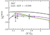 |
Fig. 4. I-band absolute magnitude of the RGB tip as a function of V-I colour. The calibration of our measurements in the SMC and LMC are plotted as yellow filled circles with vertical error-bar at 1σ confidence intervals and horizontal error-bars at 1σ confidence interval. In all cases, the point corresponding to the SMC has a bluer colour (here (V-I)0) than the one corresponding to the LMC. The grey triangle is the calibration obtained by Soltis et al. (2021) in ω Cen. The black curve is the calibration provided by H23 in form of a second order polynomial fit. The coloured curves are model predictions obtained from the set of Padua isochrones by Bressan et al. (2012), corresponding to ages of 4 Gyr (purple line), 10 Gyr (light blue), and 13 Gyr (green line), all vertically shifted by the amount reported in the plot (mod. shift). The shift is applied to make the 10 Gyr model, taken as reference, to match the point corresponding to the LMC. |
In Fig. 4, our measurements are represented as yellow filled circles, while the one from Soltis et al. (2021) for ω Cen is given by a grey filled triangle and the black curve is the quadratic polynomial relation from Jang & Lee (2017), with the ZP adjusted to match the measurements by H23 (a good synthetic representation of the H23 results over a broad colour range). It is interesting to note that in spite of the obvious difference in the ZP, the branch of the curve in the range of colours where our points are located is very flat, in excellent agreement with the virtually null difference we obtained between MITRGB of the LMC and of the SMC.
In Fig. 4, as well as in all the following analogue diagrams, we plot the theoretical predictions for the absolute magnitude of the tip as a function of colour for solar-scaled models of age 4 Gyr (purple line), 10 Gyr (light blue line), and 13 Gyr (green line). The 13 Gyr and 4 Gyr models are intended to provide a quantitative view of the amplitude of the dependency on age of the standard candle, in this case ≲0.02 mag at any colour, while the 10 Gyr model is taken as a ‘mean’ reference to give an idea of the predicted trend with colour outside the range covered by our measured points, mainly toward redder colours/higher metallicities. All the model predictions have been shifted by the amount needed to reach a match between the observed MITRGB of the LMC and the prediction of the 10 Gyr model at that colour. In the present case the shift, labelled as “mod. shift” in this kind of plot, is +0.088 mag, indicating that the predictions of PARSEC models are in better agreement with the H23 ZP and, in general, with the bright set of RGB tip calibrations, than with our calibration or of those by Soltis et al. (2021) and Li et al. (2023). In fact, they are also 0.01 mag to 0.06 mag brighter than the quadratic polynomial based on the H23 calibration, depending on the colour and age of the models. It is also worth noting that the dependency on colour of the age ≲10 Gyr models is quite different from the polynomial representing the H23 calibration, especially in the blue and metal-poor regime around the colour of the SMC. Stellar models have their own limitations that should be always considered in these kinds of comparisons.
In summary, we used a large and independent sample of LMC and SMC stars with accurate Gaia standardised VI XPSP15, state-of-the-art extinction corrections, and the distance moduli from Pietrzyński et al. (2019) and Graczyk et al. (2020), to obtain a remarkably precise measurement of MITRGB for the LMC and SMC. The comparison of our results with the most recent and most accurate calibrations presented above shows that our result is ≃0.05 mag fainter than most of them, but in agreement with others. This is what ought to be kept in mind when using the calibrations in the other photometric systems presented in Sect. 4, as it puts our measurements in the context of the relevant literature in the particular system. The comparison presented in this section should be considered as a validation and an assessment of the accuracy of the results that can be obtained with the same samples and the same methods in the other photometric systems considered here.
4. Calibration of the RGB tip in different systems
The detection of the TRGB in the LMC and SMC samples for the relevant passbands is presented in Appendix A, using diagrams fully analogous to those shown in Fig. 3 for the JKC I band. The resulting measurements of the extinction-corrected apparent magnitude of the tip in the various passbands for the LMC and the SMC, alongside the associated 1σ and 3σ confidence intervals (as defined in Sect. 3), are listed in Table 1.
Here, we show the calibration of the absolute magnitude of the RGB tip as a function of colour adopting the same arrangement as in Fig. 4 for the following magnitudes (passbands): ACS-WFC F814W, PS1 y, SDSS i and z, JWST-NIRCAM F090W, NGRST Z087, and Euclid-VIS IE. The choice of the colour was in some case natural for the general use (F606W-F814W for the ACS-WFC system) or for the availability of only two passbands enclosed in the XP spectral range (JWST-NIRCAM and NGSRT systems). For the SDSS system, we selected the g − i colour for its high sensitivity to temperature while to display the colour dependence of the tip in Euclid-VIS IE, we were forced to recur to JKC V-I colour, as IE is the only Euclid passband enclosed within the XP spectral range.
All the plots have the same scale in the y-axis, for a direct and easy comparison of the amplitude of the dependencies on colour (metallicity) and age, as predicted by the adopted set of stellar models. The only exception is the case of Euclid-VIS IE, where a larger scale was adopted to accommodate a significantly stronger dependency on colour, that is not surprising given the much bluer wavelength range of this passband with respect to all the other ones. On the other hand, the colour range has been chosen to enclose the range spanned by the 10 Gyr model for metallicity −2.0 ≤ [M/H] ≤ −0.4. The colour and the absolute magnitude of the RGB for the various passbands and for the LMC and SMC are reported in Table 2.
. Colour and absolute magnitude of the RGB tip of the MCs in different passbands alongside 1σ confidence intervals.
In the upper panel of Fig. 5, we show  as a function of (F606W − F814W)0 in the ACS-WFC system. F814W is very similar to JKC I and the results are indeed very similar to that shown in Fig. 4, above. Here we also show the comparison with the linear calibrating relation by Rizzi et al. (2007) that has a ‘bright’ ZP, similar to H23. Our measurement of
  for the LMC is compatible, within the uncertainties, with the result recently obtained by Anderson et al. (2024), who also used Gaia DR3 synthetic photometry in their analysis. In the lower panel of Fig. 5, concerning the PS1 y band, it can be appreciated that the
  difference between the SMC and the LMC broadly follows the trend predicted by the models16. The colour dependency is similar to that of the JKC I band, in the considered colour range, and the dependency on age has a similar amplitude.
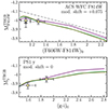 |
Fig. 5. Calibration of the RGB tip as a function of colour. Upper panel: Absolute magnitude of the RGB tip in ACS-WFC F814W band as a function of F606W-F814W colour. The dashed line is the linear calibration by Rizzi et al. (2007). Lower panel: Absolute magnitude of the RGB tip in PS1 y band as a functon of PS1 g − i colour. The meaning of the symbols and arrangement is the same as in Fig. 4. |
Figure 6 shows that SDSS i has a stronger dependency on colour than JKC I, whereas it displays the smallest amplitude of age dependency of all the passbands considered here. However, in contrast with all the other cases, the sensitivity to age is maximal in the metal-poor (blue) regime. In the lower panel of the same figure, we can appreciate the very low sensitivity of  to colour, according to the PARSEC model, over the entire colour range considered.
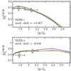 |
Fig. 6. Calibration of the RGB tip as a function of colour. Upper panel: Absolute magnitude of the RGB tip in SDSS i band as a function of SDSS g − i colour. Lower panel: Absolute magnitude of the RGB tip in SDSS z band as a function of SDSS g − i colour. The meaning of the symbols and arrangement are the same as in Fig. 4. |
JWST-NIRCAM  and NGRST
  appear similarly well-behaved, as can be appreciated from Fig. 7. It is interesting to note that in a very recent paper, Anand et al. (2024) provided a calibration of the RGB tip in the JWST-NIRCAM F090W band based on the measurement in a galaxy at D ≃ 7.6 Mpc with an available geometric distance, NGC 4258, whose mean colour of the tip is quite similar to that of the LMC17. They found
  , which is compatible with our value for the LMC
  (where the reported errorbar includes the contribution of the uncertainty in the photometric zero point; see Table 2). This provides a valuable cross-validation of the two (fully independent) calibrations in this new photometric system.
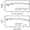 |
Fig. 7. Calibration of the RGB tip as a function of colour. Upper panel: Absolute magnitude of the RGB tip in JWST-NIRCAM F090W band as a function of F070W-F090W colour. Lower panel: Absolute magnitude of the RGB tip in NGRST Z087 band as a function of R062-Z087 colour. The meaning of the symbols and arrangement are the same as in Fig. 4. |
As expected, the dependency of MIETRGB on colour is large when the entire range spanned in Fig. 8 is considered. However, for colours bluer than the LMC tip the amplitude of the predicted trend is ≲0.1 mag and the difference in MIETRGB between the LMC and the SMC is just 0.05 ± 0.04, suggesting that it may be a good standard candle in this blue colour range.
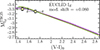 |
Fig. 8. Calibration of the RGB tip as a function of colour. Absolute magnitude of the RGB tip in Euclid-VIS IE band as a function of JKC V-I colour. The meaning of the symbols and the arrangement are the same as in Fig. 4 except for the scale of the y axis, which is wider here to accommodate for the higher amplitude of the MIETRGB trend with colour, with respect to the other passbands here. |
In general, the difference in  between SMC and LMC is never found to be statistically significant. The observed differences (SMC-LMC) are −0.13σ, −0.27σ, −0.57σ, 1.43σ, 1.47σ, 1.04σ, 0.50σ, and, −1.17σ, for JKC I, ACS-WFC F814W, SDSS i, SDSS z, PS1 y, JWST-NIRCAM F090W, NGRST Z087, and Euclid-VIS IE, respectively. In this sense, those interested in using our calibrations can take as a reference value, the
  of the galaxy, between the SMC and LMC, whichever colour is more similar to their target stellar system; alternatively, the weighted mean of the two values can be taken, if their target has colour within the range spanned by the SMC and LMC tips. To extrapolate to significantly redder colours, we can revert to models by re-adjusting the ZP to match our measurements, as described above. In cases of very weak metallicity dependency, such as
  ,
,  , or
, or  , our measurements can be taken as a reference in the entire range of colours spanned by the plots presented in this section. According to the considered models, this should lead to very small systematics, with amplitudes of the same order as the age dependency (≲0.03 mag).
In Appendix B, we provide some examples of the impact that the uncertainty in the photometric zero point may have in the total error budget18. Given the results presented in Appendix B and, in particular, the arguments presented at the end of Sect. 2, we have decided to provide (in Table 2) the total error including also the contribution of this source of uncertainty. Following the discussion in Sect. 2 (see Gaia Collaboration 2023a) we conservatively adopted a contribution from this factor of 0.01 mag for the calibrations in the JKC and SDSS systems, of 0.02 mag for the PS1 system, 0.03 mag for the HST ACS-WFC system, and 0.04 mag for the remaining (non-standardised) systems. It is worth noting that in all the considered cases, the total uncertainty on  remains ≲0.06 mag. We recommend to adopt this global error when using our calibrations, except for cases where there is a good reason not to do so; for instance, when the distance to a stellar system is derived from Gaia XP synthetic photometry, as we have done when comparing
  of the LMC and SMC. For this kind of application, we also provide in Table 2 the version of the uncertainty on
  without the contribution of the uncertainty on the photometric zero point.
The relevant point here is that in Table 2 we provide robust estimates of the absolute magnitude of the RGB tip for two fundamental pillars of the cosmological distance ladder in several suitable and widely used passbands for which such calibration was not available before. Moreover, we used one set of stellar model to provide an idea of the behaviour of the newly calibrated standard candles in colour ranges not covered by our measurements. These tools should be sufficient to get distance estimates to stellar systems with well populated RGBs with accuracy better than 5–10% in all the considered photometric systems and in a wide variety of cases.
5. Adopted tip detection algorithm
In this section, we outline the model we used to describe the RGB LF (Sect. 5.1) and the methodology employed for fitting it to a given dataset, with the aim to determine the RGB tip (Sect. 5.2). There are two types of methods for the measurement of the RGB tip given in the literature: the use of an edge detector filter (typically the Sobel’s filter, Lee et al. 1993; Madore & Freedman 1995; Sakai et al. 1996, H23) or the fitting of a simple model to the brightest portion of the RGB LF, plus an additional component accounting for AGB stars brighter than the tip and background and foreground contaminating populations (Méndez et al. 2002; Makarov et al. 2006; Conn et al. 2011, 2012, 2016). The first method, in principle, is simple and non-parametric, but the response of the edge-detector filter can be very noisy, especially in cases of sparsely populated LFs, giving rise to some ambiguity in the identification of the peak of the filter response that is actually associated with the RGB tip. Moreover, the error associated with the measurements is not well defined (see H23 for an empirical approach based on re-sampling). The second method can significantly mitigate the effects of shot noise and provides a proper quantitative description of uncertainties and covariances (see e.g. Conn et al. 2012). A potential drawback is that the measurement of mag0TRGB can be somehow influenced by the use of a model that is not flexible enough to fit simultaneously all the components of the RGB LF (e.g. its bright and faint ends, the sharpness of the transition around the tip magnitude, etc.). Here, we opted for a model-fitting technique, above all for the excellent control of the uncertainties it provides.
5.1. Model
In the adopted approach, the RGB LF, ℒRGB, in a given photometric band, is described by
where [mdown, mup] marks the bandwidth of the considered portion of the upper RGB. In Eq. (2), ℒRGB is normalised to unity and ℒσ is computed applying a Gaussian smoothing to
where the m ≥ m0TRGB branch is intended to model the AGB population. This model was previously used, for instance, by Makarov et al. (2006), Conn et al. (2012, 2016) to describe the RGB LF, in the context of the determination of the RGB tip. Therefore,
with ⊛ as the convolution operator and G a Gaussian of null mean and σTRGB dispersion. It can be shown that the analytical expression for Eq. (4) is
![$$ \begin{aligned} \begin{split} \mathcal{L} _{\sigma }(m) =&10^{a(m-m_0^\mathrm{TRGB})+c+\frac{a^2\sigma _{\rm TRGB}^2\ln 10}{2}} \times \\&\biggl [\text{ erf}\bigg (\frac{m-m_0^\mathrm{TRGB}}{\sqrt{2}\sigma _{\rm TRGB}} + \frac{a\sigma _{\rm TRGB}\ln 10}{\sqrt{2}}\biggr ) + 1\biggr ] + \\&10^{b(m-m_0^\mathrm{TRGB})+\frac{b^2\sigma _{\rm TRGB}^2\ln 10}{2}} \times \\&\biggl [1-\text{ erf}\bigg (\frac{m-m_0^\mathrm{TRGB} }{\sqrt{2}\sigma _{\rm TRGB}} + \frac{b\sigma _{\rm TRGB}\ln 10}{\sqrt{2}}\biggr )\biggr ], \end{split} \end{aligned} $$](/articles/aa/full_html/2024/11/aa49575-24/aa49575-24-eq59.gif)
where erf(x) is the error function and m0TRGB the magnitude of the RGB tip, that is the main observable quantity we want to measure.
For m ≫ m0TRGB, logℒ(m) is a power-law of slope a, while for m ≪ m0TRGB, logℒσ(m) is a power-law of slope b. The LF (3) is discontinuous at m = m0TRGB (mdown ≤ m0TRGB ≤ mup), with c describing the amplitude of the discontinuity. The use of Eq. (5) allows for a continuous modelling of the luminosity transition around the tip magnitude, but keeping the same asymptotic behaviours of model (3) for m ≪ m0TRGB and m ≫ m0TRGB.
The inclusion of the new parameter, σTRGB, is motivated by a correct modelling of the observed non-vertical luminosity drop around the tip magnitude. There are several factors that can contribute to keeping the transition a smooth function. Examples on the observational side are provided by underestimation of photometric errors and/or by the unaccounted influence of blending, both of which are expected to have negligible effects in the cases considered here. From a more physical point of view, it must be kept in mind that the tip is expected to manifest as a vertical drop in the LF for a stellar population whose stars all share the same age, metallicity, and helium abundance. However, in practical terms, within galaxies such as the ones under consideration, these parameters exhibit distributions (with correlations), which should consequently blur the actual LF cut-off corresponding to the RGB tip. Moreover, close to the tip, RGB stars may display small-amplitude variability (Wray et al. 2004) and their random-phase sampling could also contribute to tip smearing. Another significant source of broadening of the RGB tip is the possibility that the reference stellar system has a three-dimensional (3D) structure and thus a non-negligible depth. At the same luminosity, stars at the tip that are closer (further) to the observer will have a lower (higher) relative magnitude. Consequently, the overall effect of combining stars along the same line of sight but at different depths is to produce a broadening of the RGB tip. This aspect is discussed in detail in Appendix C. The five model free parameters are:
a: the power-law index for m ≫ m0TRGB;
b: the power-law index for mℒm0TRGB;
c: a measurement for the discontinuity jump around the tip magnitude;
m0TRGB: the magnitude of the tip;
σTRGB: the degree of smoothing of the LF around the tip magnitude.
In Fig. 9, we give a quantitative idea of the main role of each free parameter of model (5).
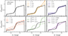 |
Fig. 9. The adopted model of the upper RGB LF (5) for different values of its free parameters. The top left panel shows a reference model (black solid line) with (a, b, c, m0TRGB, σTRGB) = (0.1, 0.3, 0.4, 14.5, 0.1) alongside the nominal value of the tip magnitude m0TRGB (vertical dashed line). The other panels show how the model changes when changing a single parameter while keeping the others to the values of the reference model. |
5.2. Method
Provided an observed set of N RGB stars sampling the RGB tip transition in a given photometric band with known magnitude, mi, and error, δmi, with i = 1, ..., N, we fit the data with model (5), thereby estimating all its parameters including m0TRGB. We employed a star-by-star fitting technique, avoiding any arbitrary binning of the data. Thus, the model likelihood is given by
where G is a Gaussian of null mean and dispersion equal to δmi. Therefore, each star is included in the fit alongside its photometric error
We conducted a Markov chain Monte Carlo (MCMC) analysis to explore the parameter space and to sample from the posterior distribution. We adopt uniform priors on the model free parameters and, to sample from the posterior, we combined the differential evolution proposal by Nelson et al. (2014) and the snooker proposal by ter Braak & Vrugt (2008), relying on the EMCEE software library (Foreman-Mackey et al. 2013). In each run, we used 30 walkers, each evolved for 5000 steps. We discarded an initial burn-in phase of at least 500 steps and implement a thinning of approximately 20 steps, aligned with the auto-correlation length of the chains. The remaining steps are used to build the posterior distributions over the model free parameters. The 1σ confidence intervals over the models parameters and any derived quantity were computed as the 16th, 50th, and 84th percentiles of the corresponding distributions, while the 3σ confidence intervals as the 0.15th, 50th, and 99.85th percentiles. Further details on the method and tests we performed to evaluate the accuracy of the algorithm are reported in Appendix E.
6. Summary and conclusions
We used Gaia DR3 synthetic photometry to assemble large selected samples of LMC and SMC stars with photometry in twenty-two optical passbands of widely used (or to be widely used in the near future) photometric systems, namely Johnson-Kron-Cousins, SDSS, PS1, HST ACS-WFC, JWST NIRCAM, NGRST, and Euclid. Having properly corrected all magnitudes for interstellar extinction, we used these samples to measure the RGB tip in both galaxies in eight suitable passbands in these photometric systems, using a fully Bayesian approach.
We coupled these measurements with the state-of-the-art distance estimates for LMC and SMC from eclipsing binaries (Pietrzyński et al. 2019; Graczyk et al. 2020) to provide calibrations of the RGB tip as a function of colour for the following eight passbands: JKC I, HST ACS/WFC F814W, SDSS i and z, PS1 y, JWST-NIRCAM F090W, NGRST Z087, and Euclid-VIS IE. The calibration in JKC I band was used for a critical comparison with other calibrations in the literature. We find that our calibration is fainter by ≃0.06 mag than that by H23 and other authors, while it is in good agreement with, for instance, the results of Soltis et al. (2021). In Appendix B, we discuss in some detail the reason of the difference with H23, highlighting the effect of a few factors that may increase uncertainties in m0TRGB and that are not always taken into account in the literature (e.g. the systematics in photometric zero points). The latter are expected to affect distance estimates obtained with all standard candles and not only the RGB tip.
We explored the behaviour of the absolute magnitude of the RGB tip as a function of colour (and age) in the various considered passbands also outside the colour range spanned by the LMC and SMC tips by means of theoretical models. Overall, SDSS z, JWST NIRCAM F090W, and NGRST Z087 appear to be the passbands where the absolute magnitude of the RGB tip displays the lowest dependency on colour, over wide colour ranges. The amplitude of the colour dependencies in these bands is similar (or slightly smaller, in some cases, for old age models) to that in JKC I.
As far as we know, in this work, we provide the first calibrations of the RGB tip in SDSS i and z, PS1 y, NGRST Z087, and Euclid-VIS IE to be published in the literature to date. An independent calibration in JWST NIRCAM F090W was recently published by Anand et al. (2024) and their result is in agreement with ours, within the uncertainties. Calibrations of the RGB tip analogous to those provided here can be obtained also for additional passbands and as a function of different colours with respect to those we adopted in the present analysis by using our LMC and SMC catalogues that we have made publicly available.
7. Data availability
Supplementary material is available at https://zenodo.org/records/10636449
The table gaiadr3.synthetic_photometry, in the Gaia Archive https://gea.esac.esa.int/archive/
These catalogues are publicly available at https://zenodo.org/records/10636449. See Appendix D for a detailed description of the content.
Advanced Camera for Surveys (ACS) Wide Field Camera (WFC) https://www.stsci.edu/hst/instrumentation/acs
The GSPC is supposed to contain also standardised PS1 y photometry but in fact, because of an error in writing the final catalogue, non-standardised PS1 y was included instead. See https://www.cosmos.esa.int/web/gaia/dr3-known-issues#SyntheticPhotSP1
The coefficients reported in Table 6 of Schlafly & Finkbeiner (2011) are valid only for non-renormalised E(B − V) values read from the original Schlegel et al. (1998) maps. We corrected them to have RV = 3.1 in Landolt’s V, making them suitable for properly scaled E(B − V) values. In this scale, RB = 4.1.
The accuracy and precision of standardised XPSP magnitudes in the UJKC and uSDSS bands are significantly less good than for these passbands. See Gaia Collaboration (2023a) for a thorough discussion.
The accuracy of XPSP as well as of any synthetic photometry depends also on the accuracy to which the transmission curves provided for the various passbands represent the real transmission curves. The standardisation process adopted by Gaia Collaboration (2023a) is intended to correct XPSP not only for systematics affecting externally calibrated XP spectra but also for inaccuracies of the adopted transmission curves.
Reproducing the JKC system photometry, as defined by Landolt’s standard stars (see Landolt & Uomoto 2007, Landolt 1992, 2007, 2009, 2013 and also Pancino et al. 2022) with an accuracy within a few millimag (Gaia Collaboration 2023a).
In the F814W-F606W colour, see Li et al. (2023).
See Gaia Collaboration (2023a) for further details on this specific XPSP standardisation.
Acknowledgments
We are very grateful to Taylor Hoyt for providing us the material for a thorough comparison with his results and for insightful discussion and to Richard Anderson for drawing our attention his very relevant paper. We appreciated some very useful suggestions from an anonymous referee. We acknowledge the help of Francesca De Angeli with GaiaXPy and Paolo Montegriffo for computing Euclid-VIS IE XPSP basis functions in the AB system. MB acknowledges the support to activities related to the ESA/Gaia mission by the Italian Space Agency (ASI) through contract 2018-24-HH.0 and its addendum 2018-24-HH.1-2022 to the National Institute for Astrophysics (INAF). M.B. acknowledges the financial support by the Italian MUR through the grant PRIN 2022LLP8TK_001 assigned to the project LEGO – Reconstructing the building blocks of the Galaxy by chemical tagging (P.I. A. Mucciarelli), funded by the European Union – NextGenerationEU. RP acknowledge the financial support to this research by the Italian Research Center on High Performance Computing Big Data and Quantum Computing (ICSC), project funded by European Union – NextGenerationEU – and National Recovery and Resilience Plan (NRRP) – Mission 4 Component 2 within the activities of Spoke 3 (Astrophysics and Cosmos Observations). This work has made use of data from the European Space Agency (ESA) mission Gaia (https://www.cosmos.esa.int/Gaia), processed by the Gaia Data Processing and Analysis Consortium (DPAC, https://www.cosmos.esa.int/web/Gaia/dpac/consortium). Funding for the DPAC has been provided by national institutions, in particular the institutions participating in the Gaia Multilateral Agreement. In this analysis we made use of TOPCAT (http://www.starlink.ac.uk/topcat/, Taylor 2005).
References
- Anand, G. S., Rizzi, L., Tully, R. B., et al. 2021, AJ, 162, 80 [CrossRef] [Google Scholar]
- Anand, G. S., Tully, R. B., Rizzi, L., Riess, A. G., & Yuan, W. 2022, ApJ, 932, 15 [NASA ADS] [CrossRef] [Google Scholar]
- Anand, G. S., Riess, A. G., Yuan, W., et al. 2024, ApJ, 966, 89 [NASA ADS] [CrossRef] [Google Scholar]
- Anderson, R. I., Koblischke, N. W., & Eyer, L. 2024, ApJ, 963, L43 [NASA ADS] [CrossRef] [Google Scholar]
- Barker, M. K., Sarajedini, A., & Harris, J. 2004, ApJ, 606, 869 [Google Scholar]
- Bedin, L. R., Cassisi, S., Castelli, F., et al. 2005, MNRAS, 357, 1038 [NASA ADS] [CrossRef] [Google Scholar]
- Bellazzini, M. 2008, Mem. Soc. Astron. It., 79, 440 [NASA ADS] [Google Scholar]
- Bellazzini, M., Ferraro, F. R., & Pancino, E. 2001, ApJ, 556, 635 [NASA ADS] [CrossRef] [Google Scholar]
- Bellazzini, M., Ferraro, F. R., Origlia, L., et al. 2002, AJ, 124, 3222 [NASA ADS] [CrossRef] [Google Scholar]
- Bellazzini, M., Ferraro, F. R., Sollima, A., Pancino, E., & Origlia, L. 2004a, A&A, 424, 199 [NASA ADS] [CrossRef] [EDP Sciences] [Google Scholar]
- Bellazzini, M., Gennari, N., Ferraro, F. R., & Sollima, A. 2004b, MNRAS, 354, 708 [NASA ADS] [CrossRef] [Google Scholar]
- Bellazzini, M., Gennari, N., & Ferraro, F. R. 2005, MNRAS, 360, 185 [NASA ADS] [CrossRef] [Google Scholar]
- Bressan, A., Marigo, P., Girardi, L., et al. 2012, MNRAS, 427, 127 [NASA ADS] [CrossRef] [Google Scholar]
- Cardelli, J. A., Clayton, G. C., & Mathis, J. S. 1989, ApJ, 345, 245 [Google Scholar]
- Choi, Y., Nidever, D. L., Olsen, K., et al. 2018, ApJ, 866, 90 [Google Scholar]
- Conn, A. R., Lewis, G. F., Ibata, R. A., et al. 2011, ApJ, 740, 69 [NASA ADS] [CrossRef] [Google Scholar]
- Conn, A. R., Ibata, R. A., Lewis, G. F., et al. 2012, ApJ, 758, 11 [Google Scholar]
- Conn, A. R., McMonigal, B., Bate, N. F., et al. 2016, MNRAS, 458, 3282 [Google Scholar]
- Cuillandre, J. C., Bertin, E., Bolzonella, M., et al. 2024, A&A, submitted, [arXiv:2405.13496] [Google Scholar]
- Cullinane, L. R., Mackey, A. D., Da Costa, G. S., Koposov, S. E., & Erkal, D. 2023, MNRAS, 518, L25 [Google Scholar]
- Da Costa, G. S., & Armandroff, T. E. 1990, AJ, 100, 162 [Google Scholar]
- De Angeli, F., Weiler, M., Montegriffo, P., et al. 2023, A&A, 674, A2 [NASA ADS] [CrossRef] [EDP Sciences] [Google Scholar]
- Dixon, M., Mould, J., Flynn, C., et al. 2023, MNRAS, 523, 2283 [NASA ADS] [CrossRef] [Google Scholar]
- Foreman-Mackey, D., Hogg, D. W., Lang, D., & Goodman, J. 2013, PASP, 125, 306 [Google Scholar]
- Freedman, W. L., Madore, B. F., Hatt, D., et al. 2019, ApJ, 882, 34 [Google Scholar]
- Fukugita, M., Ichikawa, T., Gunn, J. E., et al. 1996, AJ, 111, 1748 [Google Scholar]
- Gaia Collaboration (Prusti, T., et al.) 2016, A&A, 595, A1 [NASA ADS] [CrossRef] [EDP Sciences] [Google Scholar]
- Gaia Collaboration (Brown, A. G. A., et al.) 2021a, A&A, 649, A1 [NASA ADS] [CrossRef] [EDP Sciences] [Google Scholar]
- Gaia Collaboration (Luri, X., et al.) 2021b, A&A, 649, A7 [EDP Sciences] [Google Scholar]
- Gaia Collaboration (Montegriffo, P., et al.) 2023a, A&A, 674, A33 [CrossRef] [EDP Sciences] [Google Scholar]
- Gaia Collaboration (Vallenari, A., et al.) 2023b, A&A, 674, A1 [NASA ADS] [CrossRef] [EDP Sciences] [Google Scholar]
- Graczyk, D., Pietrzyński, G., Thompson, I. B., et al. 2020, ApJ, 904, 13 [Google Scholar]
- Hoyt, T. J. 2023, Nat. Astron., 7, 590 [NASA ADS] [CrossRef] [Google Scholar]
- Hoyt, T. J., Freedman, W. L., Madore, B. F., et al. 2018, ApJ, 858, 12 [NASA ADS] [CrossRef] [Google Scholar]
- Jang, I. S., & Lee, M. G. 2017, ApJ, 836, 74 [NASA ADS] [CrossRef] [Google Scholar]
- Landolt, A. U. 1992, AJ, 104, 340 [Google Scholar]
- Landolt, A. U. 2007, AJ, 133, 2502 [Google Scholar]
- Landolt, A. U. 2009, AJ, 137, 4186 [Google Scholar]
- Landolt, A. U. 2013, AJ, 146, 131 [Google Scholar]
- Landolt, A. U., & Uomoto, A. K. 2007, AJ, 133, 768 [Google Scholar]
- Lee, M. G., Freedman, W. L., & Madore, B. F. 1993, ApJ, 417, 553 [Google Scholar]
- Li, S., Casertano, S., & Riess, A. G. 2022, ApJ, 939, 96 [NASA ADS] [CrossRef] [Google Scholar]
- Li, S., Casertano, S., & Riess, A. G. 2023, ApJ, 950, 83 [NASA ADS] [CrossRef] [Google Scholar]
- Lindegren, L., Klioner, S. A., Hernández, J., et al. 2021, A&A, 649, A2 [EDP Sciences] [Google Scholar]
- López-Sanjuan, C., Vázquez Ramió, H., Xiao, K., et al. 2024, A&A, 683, A29 [NASA ADS] [CrossRef] [EDP Sciences] [Google Scholar]
- Madore, B. F., & Freedman, W. L. 1995, AJ, 109, 1645 [NASA ADS] [CrossRef] [Google Scholar]
- Madore, B. F., & Freedman, W. L. 2020, AJ, 160, 170 [NASA ADS] [CrossRef] [Google Scholar]
- Madore, B. F., Freedman, W. L., Owens, K. A., & Jang, I. S. 2023, AJ, 166, 2 [NASA ADS] [CrossRef] [Google Scholar]
- Magnier, E. A., Schlafly, E. F., Finkbeiner, D. P., et al. 2020, ApJS, 251, 6 [NASA ADS] [CrossRef] [Google Scholar]
- Maíz-Apellániz, J., Cieza, L., & MacKenty, J. W. 2002, AJ, 123, 1307 [Google Scholar]
- Makarov, D., Makarova, L., Rizzi, L., et al. 2006, AJ, 132, 2729 [NASA ADS] [CrossRef] [Google Scholar]
- Martin, N. F., Starkenburg, E., Yuan, Z., et al. 2024, A&A, in press, https://doi.org/10.1051/0004-6361/202347633 [Google Scholar]
- Méndez, B., Davis, M., Moustakas, J., et al. 2002, AJ, 124, 213 [CrossRef] [Google Scholar]
- Montegriffo, P., De Angeli, F., Andrae, R., et al. 2023, A&A, 674, A3 [NASA ADS] [CrossRef] [EDP Sciences] [Google Scholar]
- Murray, C. E., Hasselquist, S., Peek, J. E. G., et al. 2024, ApJ, 962, 120 [NASA ADS] [CrossRef] [Google Scholar]
- Nardiello, D., Libralato, M., Piotto, G., et al. 2018, MNRAS, 481, 3382 [NASA ADS] [CrossRef] [Google Scholar]
- Nelson, B., Ford, E. B., & Payne, M. J. 2014, ApJS, 210, 11 [Google Scholar]
- Omkumar, A. O., Subramanian, S., Niederhofer, F., et al. 2021, MNRAS, 500, 2757 [Google Scholar]
- Pancino, E., Marrese, P. M., Marinoni, S., et al. 2022, A&A, 664, A109 [NASA ADS] [CrossRef] [EDP Sciences] [Google Scholar]
- Pietrzyński, G., Graczyk, D., Gallenne, A., et al. 2019, Nature, 567, 200 [Google Scholar]
- Riello, M., De Angeli, F., Evans, D. W., et al. 2021, A&A, 649, A3 [NASA ADS] [CrossRef] [EDP Sciences] [Google Scholar]
- Rizzi, L., Tully, R. B., Makarov, D., et al. 2007, ApJ, 661, 815 [Google Scholar]
- Sakai, S., Madore, B. F., & Freedman, W. L. 1996, ApJ, 461, 713 [Google Scholar]
- Salaris, M., & Cassisi, S. 1998, MNRAS, 298, 166 [NASA ADS] [CrossRef] [Google Scholar]
- Saltas, I. D., & Tognelli, E. 2022, MNRAS, 514, 3058 [NASA ADS] [CrossRef] [Google Scholar]
- Schlafly, E. F., & Finkbeiner, D. P. 2011, ApJ, 737, 103 [Google Scholar]
- Schlegel, D. J., Finkbeiner, D. P., & Davis, M. 1998, ApJ, 500, 525 [Google Scholar]
- Scolnic, D., Riess, A. G., Wu, J., et al. 2023, ApJ, 954, L31 [NASA ADS] [CrossRef] [Google Scholar]
- Serenelli, A., Weiss, A., Cassisi, S., Salaris, M., & Pietrinferni, A. 2017, A&A, 606, A33 [NASA ADS] [CrossRef] [EDP Sciences] [Google Scholar]
- Skowron, D. M., Skowron, J., Udalski, A., et al. 2021, ApJS, 252, 23 [Google Scholar]
- Soltis, J., Casertano, S., & Riess, A. G. 2021, ApJ, 908, L5 [Google Scholar]
- Tatton, B. L., van Loon, J. T., Cioni, M. R. L., et al. 2021, MNRAS, 504, 2983 [NASA ADS] [CrossRef] [Google Scholar]
- Taylor, M. B. 2005, ASP Conf. Ser., 347, 29 [Google Scholar]
- ter Braak, C., & Vrugt, J. 2008, Stat. Comput., 18, 435 [CrossRef] [Google Scholar]
- Thanjavur, K., Ivezić, Ž., Allam, S. S., et al. 2021, MNRAS, 505, 5941 [NASA ADS] [CrossRef] [Google Scholar]
- Thompson, I. B., Kaluzny, J., Pych, W., et al. 2001, AJ, 121, 3089 [NASA ADS] [CrossRef] [Google Scholar]
- Udalski, A., Soszynski, I., Szymanski, M. K., et al. 2008a, Acta Astron., 58, 89 [NASA ADS] [Google Scholar]
- Udalski, A., Soszyński, I., Szymański, M. K., et al. 2008b, Acta Astron., 58, 329 [NASA ADS] [Google Scholar]
- Valenti, E., Ferraro, F. R., & Origlia, L. 2004, MNRAS, 354, 815 [NASA ADS] [CrossRef] [Google Scholar]
- Wray, J. J., Eyer, L., & Paczyński, B. 2004, MNRAS, 349, 1059 [Google Scholar]
- Wu, J., Scolnic, D., Riess, A. G., et al. 2023, ApJ, 954, 87 [NASA ADS] [CrossRef] [Google Scholar]
- Xiao, K., Yuan, H., Huang, B., et al. 2023, ApJS, 268, 53 [NASA ADS] [CrossRef] [Google Scholar]
- Yuan, W., Riess, A. G., Macri, L. M., Casertano, S., & Scolnic, D. M. 2019, ApJ, 886, 61 [Google Scholar]
- Zivick, P., Kallivayalil, N., & van der Marel, R. P. 2021, ApJ, 910, 36 [Google Scholar]
Appendix A: Detection of the RGB tip in different passbands
In Fig. A.1 and Fig. A.2, the detection of the RGB tip in the SMC and LMC are shown for the various passbands considered here in addition to JKC I (see Sect. 3). The arrangement and the meaning of the symbols are the same as in Fig. 3. The detection is fairly clean in all the considered cases.
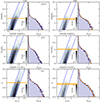 |
Fig. A.1. Detection of the TRGB with our method for the LMC (left column of panels) and the SMC (right column of panels), for, from the upper to the lower row of panels, JWST-NIRCAM F090W, ACS-WFC F814W, and yPS1 passbands, as a function of a colour in the respective photometric systems. The arrangement and the meaning of the symbols are the same as in Fig. 3. |
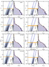 |
Fig. A.2. Detection of the TRGB with our method for the LMC (left column of panels) and the SMC (right column of panels), for, from the upper to the lower row of panels, SDSS i, SDSS z, NGRST (WFIRST) Z087 and Euclid-VIS IE passbands, as a function of a colour in the respective photometric systems (except for Euclid, as IE is the only passband of the system that is completely enclosed in the spectral range of Gaia XP spectra; in this case we used the V-I colour). The arrangement and the meaning of the symbols are the same as in Fig. 3. |
Appendix B: The origin of the differences with H23 and the excellent match with Y99
In Sect. 3, we show that our measurements of the extinction-corrected apparent magnitudes of the JKC I band RGB tip of the LMC and SMC are ≃0.06 mag fainter than the corresponding state-of-the-art measurements by H23. In this appendix, we try to understand the reason for this difference by exploring a few possibly promising hypotheses.
First, it has to be noted that in H23 the detection of the RGB tip is obtained with the edge-detector filter technique while here we adopted the model fitting (MF) method described in Sect. 5.2. In principle, there is no guarantee that the two methods locate the tip exactly at the same position (Anand et al. 2022, 2024; Anderson et al. 2024). To test this possibility we repeated all the RGB tip detections presented in Sect. 3 and Appendix A using the Sobel filter technique (Sakai et al. 1996) exactly on the same samples of colour selected RGB and AGB stars. In all the cases the TRGB was unambiguously identified as a dominant peak in the filter response. We assumed the half width at half maximum (HWHM) of the filter response peak associated with the tip as the uncertainty on the magnitude of the tip. This is probably an overestimate of the actual uncertainty but it is a simple and well defined quantity. Moreover, here we are mainly interested to check if there is a systematic difference between the two methods in the actual location of the tip. The upper panel of Fig. B.1 shows the comparison between the magnitude of the tip obtained from the two different techniques for the sixteen cases considered in this paper (8 passbands × 2 samples). All the points lie very close to the mag mag
mag line and the residuals (magSTRGB-mag
 ), plotted in the lower panel of the figure, are strongly clustered around zero, with a mean as small as +0.004 mag and a standard deviation of 0.018 mag, with no obvious sign of systematics. From this experiment we can conclude that it is very unlikely that the detection method is responsible for the difference between our estimates of the MC tips and those by H23, but also that there is an unavoidable amount statistic uncertainty intrinsically associated with the way in which the measurement is performed, here of order of 0.02 mag (Anand et al. 2022). The RGB tip is a somehow anomalous standard candle, where the reference observable is not, for instance, the mean magnitude of any individual source of a given class but, instead, a collective property of a stellar population that must be inferred, hence it is not surprising that the inference method can play a role in the reproducibility of measurements. It is important to be aware that this limit in accuracy is inherent to each measurement of the tip even if it is generally neglected19. In the specific case of the JKC I band for the LMC the measure obtained with the Sobel filter is 0.012 mag brighter than that obtained with the MF algorithm. Hence, a small part of the difference between us and H23 in I0TRGB for this galaxy can be ascribed to a ≃1σ fluctuation in this intrinsic term of the uncertainty budget.
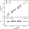 |
Fig. B.1. Comparison between the magnitudes of the TRGB in the LMC (blue filled squares) and in the SMC (orange filled pentagons) in all the considered passbands measured with the MF algorithm (mag |


A second issue that we explore is the detailed selection of the sample adopted for the detection, in particular for the LMC. H23 used the Voronoi tessellation of the OGLE-III sample obtained in Hoyt et al. (2018) and made a detailed analysis to select the bins ensuring the most precise detection of the LMC tip. To check if differences in the adopted sample is at the origin of the differences in the tip measures we repeated the tip detection for the LMC using the stars in our sample enclosed in the same five Voronoi bins selected by H23. Moreover we adopted the same correction for the inclination of the LMC disc used by H2320. The detection of the tip with this sub-sample is shown in Fig. B.2. We confirm that the detection in this sample is especially clean and more precise that in the entire sample we used elsewhere. For instance, the HWHM of the peak in the Sobel filter response is ±0.040 mag for the tip detection with this subsample and  for the detection with the entire sample.
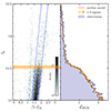 |
Fig. B.2. Detection of the RGB tip in the JKC I band for the LMC adopting only stars lying within the Voronoi bins used by H23 for his calibration. The arrangement and the meaning of the symbols are the same as in Fig. 3. |
The actual measure of the tip with the MF method for the H23 selected sample is  to be compared to
  for the entire sample. The difference is < 3σ but it goes in the direction of reconciling our measure with that by H23. Still, the amplitude of the effect (0.02 mag) is not sufficient to fill the observed gap between the two measures (0.06 mag).
Finally, we compared the photometric zero points. In Fig. B.3 we show the distribution of the difference in I magnitudes between OGLE-III photometry and our XP standardised synthetic photometry for the stars in common between the two datasets in the LMC and SMC, as a function of V-I colour. In both cases, OGLE-III I band magnitudes display a photometric zero point brighter by 0.02-0.03 mag than that of our Gaia XPSP sample. Also this difference goes in the direction of reconciling the two sets of RGB tip measures, in this case by correcting H23 measures toward fainter magnitudes. Also in this case, the amplitude of the effect does not seem sufficient to close the gap. It is worth noting that the general trends with colour shown in Fig. B.3 hide trends with position in the sky that are mapped in Fig. B.4 for the LMC, as an example. In this plot each healpix is coloured according to the median of the distribution of the ΔI = IOGLE3 − IXPSP difference for the stars in the healpix, after removing from the sample all the extreme outliers having |ΔI|> 1.0 mag. Both large and small scale trends with typical amplitude ≲0.04 mag are apparent. The fact that they correlate clearly with the tiling pattern of OGLE-III strongly suggest that XPSP is the most precise source of photometry in this comparison.
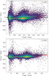 |
Fig. B.3. Difference between I magnitudes from our XPSP samples and OGLE-III for 315080 stars in common between the two samples having |ΔI|< 1.0 (LMC; upper panel) and 90115 stars in common between the two samples having |ΔI|< 1.0 (SMC; lower panel). In each panel, the red line is the median difference computed in bins 0.2 mag wide. |
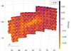 |
Fig. B.4. LMC healpix map (HEALPiX level 10) obtained from the same subsample of stars in common between out XPSP sample and the OGLE III sample adopted in Fig. B.3. The pixels are coloured according the median difference IOGLE3 − IXPSP. |
Indeed Gaia Collaboration (2023a) showed that XPSP reproduces the Landolt’s incarnation of the JKC system in I band with a typical accuracy < 3.0 mmag and precision of ≃10 mmag, in the range 11.0 < G < 17.5. Moreover XPSP photometry displays a remarkable uniformity all over the sky (see e.g. Montegriffo et al. 2023), and is being widely used as a reference to obtain more consistent photometric calibrations of existing surveys (see e.g. Martin et al. 2024; Xiao et al. 2023; López-Sanjuan et al. 2024).
This last comparison highlights a general issue that may affect all standard candles: state-of-the-art photometric datasets (in particular ground-based ones) may have inconsistencies in the photometric zero points at the 2-3% level, including trends with colour and/or position in the sky. The effects of this generally neglected source of uncertainty can be significantly mitigated, at least for the photometric systems standardised by Gaia Collaboration (2023a), by the availability of the all-sky Gaia XPSP, providing, in practice, a reliable and dense grid of standard stars to which all photometric observations can be referred.
Comparison with Yuan et al. (2019)
In this section, we briefly illustrate how the same kind of difference in the photometric zero point that mitigates the mismatch between our calibration of MITRBG for the LMC with that by H93, may act to worsen the (apparently) nearly perfect match with that by Y19, who finds MITRBG = −3.970 ± 0.046, formally within 0.007 mag of our value. In Fig. B.5 we show that the Y99 F814W photometric scale is ≃0.03 mag brighter than our XPSP in the same passband, approximately corresponding to ≃0.04 mag in IJKC band. This translates into a difference in the same sense but slightly larger than that found with OGLE3, in good agreement with the comparison between OGLE3 and Y19 photometry presented in Y19.
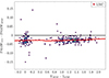 |
Fig. B.5. Difference between F814W magnitudes from our XPSP LMC sample and Y19 for 316 stars in common, as a function of V-I colour. The red line is the median difference computed in bins 0.3 mag wide. The vertical scale and the overall arrangment of the plot are the same as in Fig. B.3 to allow a direct comparison. |
If we correct the Y19 MITRBG value by this photometric shift, the difference between our LMC calibration and theirs inflates to −0.05 ± 0.06, still not significant but much larger than comparing only the final calibrated values. This exercise may serve as an additional example of the possible role of the uncertainty in the photometric zero points in the use of standard candles for distance determination.
The photometric zero point difference that we detect here between Gaia XPSP and Y99 photometry in F814W probably implies a difference in zero point between Y99 and the reference photometry we used to standardise XPSP in the ACS/WFC system (Nardiello et al. 2018)21. This should not come as a strong surprise, since, while the photometric precision achievable with HST is tipically exquiste, the calibration of individual photometric sets into the absolute scale may be subject to various sources of uncertainty. For example, according to the detailed study by Bedin et al. (2005), the simple correction of the conventional r = 0.5″ aperture to infinity is associated with an uncertainty as large as 0.015 mag. To account for this factor and given the results of the comparison presented here, in the error budget that includes the uncertainty in the photometric zero point in Table 2 we adopted a 3% additional uncertainty on the  calibration.
Appendix C: Selection and geometric effects
One drawback of using the Magellanic Clouds as the basis for the calibration of standard candles is that both galaxies display a 3d structure that, given their relatively closeness to us, has non-negligible impact on the apparent magnitude of the candles. The main body of LMC is a thick disc with relatively low inclination (i ≃ 33°; Gaia Collaboration 2021b), such that the NE edge is ∼4 kpc closer to us than the opposite SW edge (see Gaia Collaboration 2021b, and references therein). Moreover, it has been suggested that the disc is warped in its outskirts (beyond R ≃ 7.0°, according to Choi et al. 2018). On the other hand, the SMC is known to be significantly elongated along the line of sight, but with an irregular structure, probably due to tidal interactions with the LMC (Omkumar et al. 2021; Tatton et al. 2021; Zivick et al. 2021; Cullinane et al. 2023, and references therein). Murray et al. (2024) recently presented evidence supporting the idea that what we call SMC is in fact the superposition of two bodies located at slightly different distances along the same line of sight, and displaying different internal kinematics.
A detailed modelling of the 3d structure of the LMC and SMC is clearly beyond the scope of the present contribution. Our approach is to try to average out these effects by the adoption of large samples with an approximately uniform distribution in azimuth and including a parameter (σTRGB; Sect. 5.2) in the model used to detect the RGB Tip that can account for any effects that can contribute to smear out the Tip signal, including dispersion due to geometrical 3d structure. However it is worth inspecting the typical size of these effects.
For the LMC, in Fig. C.1 we show the RGB detection in IJKC on sub-samples from the various quadrants and from an inner and outer radial region. X and Y are orthographic projection coordinates in degrees computed according to Eq. 1 by Gaia Collaboration (2021b). Each quadrant provide approximately the same contribution, in number of stars, to the entire sample and the inner and outer sub-samples have similar dimension by intentional choice of the dividing radius. Finally we also report the detection obtained for the entire sample, for reference. The analysis described above is made on the LMC sample as it is and also after correcting it for the disc inclination, using Eq. 5 of H23 with the model parameters taken from Gaia Collaboration (2021b).
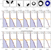 |
Fig. C.1. Upper row of panels: maps of the stars in the different subsamples of the LMC samples used for the RGB Tip detections shown in the lower panels. The inclination of the LMC disc is such that the NE side is the closest to us and the SW side is the farthest. Middle row of panels: Detection of the RGB Tip in different quadrants (four leftmost panels) and different radial zones (fifth and sixth panels from the left) of the LMC sample. In the eighth panel the detection on the entire sample is shown. Lower row of panels: the same as in the middle raw but after applying the correction for the 3d geometry of the LMC. |
The detections in the various quadrants in the original sample clearly show the significant impact of the 3d structure of the galaxy in our sample, that is dominated by stars outside the LMC centre, where the effects of the disc orientation along the line of sight are more significant. Indeed, the distance difference inferred from the RGB tip difference between the SW and NE quadrants is ≃3.7 kpc. The simple model adopted to correct for the 3d structure of the disc significantly mitigates these difference, reducing the maximum distance difference between quadrants to ≃1.9 kpc, within the range of the 3σ uncertainty (neglecting the contribution to the error budget of the photometric zero point, as here this is the same for all the detections). The differences between the detections in the inner and outer sub-samples are relatively small in both cases (+0.038 mag in the original sample and +0.019 mag in the corrected sample). However, the most interesting comparison shown in Fig. C.1 is that between the detections on the entire sample: the difference in I0TRGB between the original and the corrected samples is a mere −0.015 ± 0.008 mag, the two detections having similar uncertainties. This demonstrate that our strategy of averaging out on the 3d structure has been successful, at least in this case. It is also interesting to note that σTRGB is 20% larger in the detection from the original sample than in that in the corrected one, suggesting that this parameter can properly take into account smearing effects like those due to the 3d structure of stellar systems.
Since no simple model is available to attempt a correction for the 3d structure of the SMC, we simply repeat the above analysis for the original SMC sample, to gauge the amplitude of the differences in the measurement of the tip as a function of azimuth and angular distance from the centre of the galaxy. The results are displayed in Fig. C.2. The comparison between the various quadrants indeed reveals a complex structure both in term of mean distance, with differences up to +0.158 ± 0.040 mag in  (between the SW and the NE quadrants), and, presumably, in term of depth along the line of sight, with differences in the σTRGB parameter up to 0.114 ± 0.035 mag (between the NE and the NW quadrants).
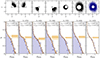 |
Fig. C.2. Upper row of panels: Maps of the stars in the different subsamples of the SMC samples used for the RGB Tip detections shown in the lower panels. Lower row of panels: Detection of the RGB Tip in different quadrants (four leftmost panels) and different radial zones (fifth and sixth panels from the left) of the LMC sample. In the eighth panel the detection on the entire sample is shown. |
The SW quadrant, having the largest  value is also the most populated one, while the NE quadrant is the least populated one. It is hard to say if this unbalance may produce a bias with respect to the (unknown) mean distance of the SMC. However we verified that the mean of the tip measurements of the four quadrants weighted by the number of stars,
  , matches very well with the measurements obtained from the entire sample,
  , hence we can evaluate the impact of the various quadrants on the final mean in a simple way. If we remove the SW quadrant from the weighted mean we obtain a
  value brighter by 0.037 mag, if we remove the NE quadrant we obtain a
  value fainter by 0.024 mag. Hence, in spite of the different sample size, the contribution of the two most extreme quadrants compensates in the determination of
  from the total sample at the ≃0.01 mag level. The 0.049 mag difference in
  between the inner and outer halves of the SMC sample is mainly driven by the asymmetry of the adopted selection. This implies that the inner sample is mainly populated by stars from the SW quadrant, driving the tip to faintest magnitudes with respect to the outer sample. In this context, the approach of averaging out all these differences into a global measurement appears as a simple, sensible choice, keeping in mind that the highly irregular 3d structure of the SMC may add some uncertainty to our calibration.
Appendix D: Value-added LMC and SMC catalogues
The photometric catalogues on which the present study is based are made publicly available as binary fits tables that can be retrieved from https://zenodo.org/records/10636449, one for the LMC (603311 stars) and one for the SMC (124578 stars). The way in which the stars to be included in the catalogues have been selected as well as how it has been obtained the E(B-V) value associated with each star are described in detail in Sect. 2.
Each catalogue contains:
-
Column 1-15: parameters directly extracted from the Gaia DR3 source catalogue22, namely: source_id, ra, dec, parallax, parallax_error, pmra, pmra_error, pmdec, pmdec_error, ruwe, phot_variable_flag, and non_single_star.
-
Column 16: C⋆, a parameter that is derived from phot_bp_rp_excess_factor (that, in turn, has been extracted from the Gaia DR3 source catalogue) following (Riello et al. 2021).
-
Column 17: colour excess E(B-V), derived from Skowron et al. (2021) and Schlegel et al. (1998), Schlafly & Finkbeiner (2011) as described in Sect. 2.
-
Columns 18-27: standardised ugriz magnitudes in the SDSS system extracted from the Gaia DR3 GSPC (Gaia Collaboration 2023a) and associated uncertainties.
-
Columns 28-37: standardised UBVRI magnitudes in the JKC system extracted from the Gaia DR3 GSPC (Gaia Collaboration 2023a) and associated uncertainties.
-
Columns 38-47: standardised grizy magnitudes in the PS1 system computed with GaiaXPy and associated uncertainties.
-
Columns 48-51: standardised F606W, F814W magnitudes in the HST ACS-WFC system extracted from the Gaia DR3 GSPC (Gaia Collaboration 2023a) and associated uncertainties.
-
Columns 52-55: non-standardised F070W and F090W magnitudes in the JWST-NIRCAM system computed with GaiaXPy and associated uncertainties.
-
Columns 56-59: non-standardised R062 and Z087 magnitudes in the NGRST system computed with GaiaXPy and associated uncertainties.
-
Columns 60-61: non-standardised IE (Cuillandre et al. 2024) magnitude in the Euclid system computed with GaiaXPy and associated uncertainties (in this case, not corrected for the bias described in Sect. 2.1 of Gaia Collaboration 2023a, hence slightly underestimated).
It is very important to remind that uSDSS and UJKC magnitudes from Gaia XPSP are significantly less accurate and precise than all the other magnitudes included in our catalogues (see Gaia Collaboration 2023a, for detailed discussion). Each star can lack some of the 22 magnitudes listed in the catalogues, depending on the signal-to-noise constraints applied to the original GSPC (S/N> 30 Gaia Collaboration 2023a). For example, of the 603311 stars listed in the LMC sample only 83229(85338) have valid uSDSS(UJKC) magnitudes.
The catalogues can be useful for several applications, like, for example, to replicate the analysis presented here, to obtain calibrations of the RGB tip in passbands (or as a function of colours) not considered here, for careful selection of targets for spectroscopic follow-up, and to test stellar models in different photometric systems.
Appendix E: Details on the RGB tip fitting procedure
Fig. E.3 shows two examples of one- and two-dimensional posterior distributions (cornerplots) of the model free parameters when fitting the RGB LF in the JKC passband for the SMC (left) and the LMC (right). In all other cases, the cornerplots are very similar to those shown in Fig. E.3, and we do not show them here for the sake of brevity. All parameters are well-constrained, with the RGB tip magnitude m0TRGB exhibiting weak correlation with the other parameters. The most correlated parameters are always the slope b and the discontinuity jump c. This dependence is easily understood, as a slight change in slope can compensate for a narrower/broader magnitude discontinuity when convolved by σTRGB. For all passbands and both galaxies, in Table E.2 we list the model median parameters alongside the 1σ confidence intervals resulting from the fitting procedure (see also Fig.s A.1 and A.2).
We tested the robustness of the tip estimate against variations of the adopted portion of the upper RGB LF included in the fit, against the number of stars in the sample for a fixed magnitude range, and the effect of introducing σTRGB over a model with σTRGB = 0. All tests were performed using the SMC sample in the JKC photometric system, though we expect similar trends in the LMC and in different photometric bands.
Specifically, the tests considered are as follows:
-
i)
1000 stars between 14 and 16 mag;
-
ii)
5000 stars between 14 and 16 mag;
-
iii)
All stars between 14.5 and 15.5 mag;
-
iv)
All stars between 14.5 and 16 mag;
-
v)
All stars between 14 and 15.5 mag;
-
vi)
All stars between 14 and 16 mag (the reference model);
-
vii)
All stars between 14 and 16.5 mag;
-
viii)
All stars between 14 and 16 mag but with σTRGB = 0.
Figure E.1 and Table E.1 schematically present the outcomes of our analysis, displaying the inferred values of the model parameters for all the considered cases. The errors are computed consistently with our definition. Below, we provide a few key observations:
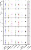 |
Fig. E.1. Tests performed on SMC sample in the JKC band (see Appendix E). The panels, from top to bottom, show the inferred models parameters m0TRGB, σTRGB, a, b and c, alongide the 1σ and 3σ confidence intervals in the cases considered. |
Results of the tests performed on the SMC sample in the JKC band (see Appendix E for details). The table reports, from left to right, the 1σ and 3σ values of m0TRGB, σTRGB, a, b, and c, while from top to bottom, lists the different tests.
1σ confidence intervals on the model free parameters as a result of the fitting algorithm of Sect. 5.2. From left to right: target galaxy (SMC or LMC), photometric system, magnitude, a, b, c, m0TRGB and σTRGB from model 5.
– Effect of sample size: as it is reasonable to expect, using fewer stars within a fixed magnitude range results in larger errors in the model parameters (e.g. blue and orange points to the left in Fig. E.1).
– effect of magnitude range: considering all stars within ±0.5 mag from the tip (i.e. a magnitude range of 14.5-15.5) results in the most uncertain estimates for parameters a, b, and c. The estimate for a improves when the magnitude range is increased towards higher magnitudes (14.5-16), while the estimate for b improves when the magnitude range is extended towards lower magnitudes (14-15.5). Both estimates improve simultaneously when the magnitude range is 14-16. This result is expected since a is sensitive to the less luminous end and b to the more luminous end of the RGB LF, necessitating adequate sampling of these regions for accurate parameter constraints. When considering even wider magnitude ranges (14-16.5), the inference for the slope a continues to improve, but there is no significant gain for the other parameters. Notably, the median tip magnitude and its corresponding errors remain approximately the same. This indicates that fitting broader portions of the LF does not improve the estimate of the tip. The precision of the tip estimate depends primarily on how well the tip itself is sampled, rather than the width of the LF included in the fit.
– consistency of tip measurements: in all cases considered, the tip measurements are consistent within the errors, despite variations in the estimates of other parameters.
– effects of σTRGB: the last case is intended to test whether the introduction of σRGBT introduces biases in the estimate of the tip magnitude. This is done by consistently fitting the same reference case (SMC in the JKC passband) with a σRGBT = 0 model (pink points to the right of Fig. E.1). All parameters, except for m0TRGB, show variations that are, within the errors, relatively inconsistent with the corresponding model with σTRGB. On the other hand, the inferred tip magnitude remains within < 1.6σ of our reference value obtained with a model that includes σTRGB, demonstrating that this parameter does not bias the measurement.
We note that introducing σTRGB to the model yields a more realistic errors representation on m0TRGB and larger errors on all other parameters. When σRGBT = 0, the error on m0TRGB shrinks to the order of the photometric error (0.005 mag), hence it is clearly underestimated. Although this could be interpreted as a very precise measurement of the tip, a close look to a comparison between data and model is enough to notice that this model gives an erroneous representation of the RGB LF. This lack of flexibility is the reason to the unrealistically small errors on the tip: when the LF presents a smooth transition and a broad RGB tip, a model with σTRGB = 0 is simply inadequate to accurately represent the data. Fig E.2 shows the SMC RGB LF in the JKC alongside the median model and the 1 − 3σ confidence interval of the σTRGB = 0 case. Due to this lack of flexibility, the model is strongly constrained around values that are not representative of the LF and is incapable of exploring better-fitting models, resulting in a statistically precise measurement, but inadequate error estimation.
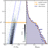 |
Fig. E.2. Detection of the RGB tip in the JKC I band for the SMC fitting a model with σTRGB = 0. The value of the model parameters and errors are listed to the bottom of Table E.1. |
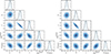 |
Fig. E.3. Examples of two- and one-dimensional marginalised posterior distributions on the model free parameters for the SMC (left) and LMC (right) in the JKC passbands (see also Sect. 3). The vertical dashed-blue lines in the one-dimensional distributions show the 16th, 50th and 84th percentiles used to evaluate the parameters 1σ confidence intervals. |
Our choice to standardize to a range of 1.5 to 2 magnitudes around the tip is motivated by model convergence and the need to ensure adequate sampling of the RGB LF. We avoided considering larger magnitude ranges (such as 14 to 16.5 in the SMC) to reduce computational time. In the case of the LMC, a 2.5 magnitude range results in a significantly high number of stars, which sensibly slows down the fitting process without improving the accuracy of the tip estimate.
All Tables
. Colour and absolute magnitude of the RGB tip of the MCs in different passbands alongside 1σ confidence intervals.
Results of the tests performed on the SMC sample in the JKC band (see Appendix E for details). The table reports, from left to right, the 1σ and 3σ values of m0TRGB, σTRGB, a, b, and c, while from top to bottom, lists the different tests.
1σ confidence intervals on the model free parameters as a result of the fitting algorithm of Sect. 5.2. From left to right: target galaxy (SMC or LMC), photometric system, magnitude, a, b, c, m0TRGB and σTRGB from model 5.
All Figures
|
Fig. 1. Distribution in the sky of the stars in our LMC sample (left panel) and SMC sample (right panel). Stars are colour-coded according to the local surface density. Stars excluded from the sample used for the detection of the RGB tip are plotted in grey-scale, while those retained are plotted in Viridis scale. |
| In the text | |
|
Fig. 2. CMD of the stars in our LMC sample (left panel) and SMC sample (right panel) in the Gaia DR3 photometric system. The meaning of symbols and colours is the same as in Fig. 1. |
| In the text | |
|
Fig. 3. Measuring the RGB tip in JKC I band in the LMC (left pair of panels) and in the SMC (right pair of panels). The left panels of each pair display the CMD of the considered sample with the selection of the RGB + AGB sub-sample that is later used to construct the LF (stars enclosed within the blue parallel lines). The orange horizontal line marks the position of the RGB tip and the shaded bands show the 1σ and 3σ confidence intervals. The right panels of each pair show the LF of the selected RGB + AGB sub-sample (light-blue histogram) and the best-fit model which we used to estimate ITRGB. |
| In the text | |
|
Fig. 4. I-band absolute magnitude of the RGB tip as a function of V-I colour. The calibration of our measurements in the SMC and LMC are plotted as yellow filled circles with vertical error-bar at 1σ confidence intervals and horizontal error-bars at 1σ confidence interval. In all cases, the point corresponding to the SMC has a bluer colour (here (V-I)0) than the one corresponding to the LMC. The grey triangle is the calibration obtained by Soltis et al. (2021) in ω Cen. The black curve is the calibration provided by H23 in form of a second order polynomial fit. The coloured curves are model predictions obtained from the set of Padua isochrones by Bressan et al. (2012), corresponding to ages of 4 Gyr (purple line), 10 Gyr (light blue), and 13 Gyr (green line), all vertically shifted by the amount reported in the plot (mod. shift). The shift is applied to make the 10 Gyr model, taken as reference, to match the point corresponding to the LMC. |
| In the text | |
|
Fig. 5. Calibration of the RGB tip as a function of colour. Upper panel: Absolute magnitude of the RGB tip in ACS-WFC F814W band as a function of F606W-F814W colour. The dashed line is the linear calibration by Rizzi et al. (2007). Lower panel: Absolute magnitude of the RGB tip in PS1 y band as a functon of PS1 g − i colour. The meaning of the symbols and arrangement is the same as in Fig. 4. |
| In the text | |
|
Fig. 6. Calibration of the RGB tip as a function of colour. Upper panel: Absolute magnitude of the RGB tip in SDSS i band as a function of SDSS g − i colour. Lower panel: Absolute magnitude of the RGB tip in SDSS z band as a function of SDSS g − i colour. The meaning of the symbols and arrangement are the same as in Fig. 4. |
| In the text | |
|
Fig. 7. Calibration of the RGB tip as a function of colour. Upper panel: Absolute magnitude of the RGB tip in JWST-NIRCAM F090W band as a function of F070W-F090W colour. Lower panel: Absolute magnitude of the RGB tip in NGRST Z087 band as a function of R062-Z087 colour. The meaning of the symbols and arrangement are the same as in Fig. 4. |
| In the text | |
|
Fig. 8. Calibration of the RGB tip as a function of colour. Absolute magnitude of the RGB tip in Euclid-VIS IE band as a function of JKC V-I colour. The meaning of the symbols and the arrangement are the same as in Fig. 4 except for the scale of the y axis, which is wider here to accommodate for the higher amplitude of the MIETRGB trend with colour, with respect to the other passbands here. |
| In the text | |
|
Fig. 9. The adopted model of the upper RGB LF (5) for different values of its free parameters. The top left panel shows a reference model (black solid line) with (a, b, c, m0TRGB, σTRGB) = (0.1, 0.3, 0.4, 14.5, 0.1) alongside the nominal value of the tip magnitude m0TRGB (vertical dashed line). The other panels show how the model changes when changing a single parameter while keeping the others to the values of the reference model. |
| In the text | |
|
Fig. A.1. Detection of the TRGB with our method for the LMC (left column of panels) and the SMC (right column of panels), for, from the upper to the lower row of panels, JWST-NIRCAM F090W, ACS-WFC F814W, and yPS1 passbands, as a function of a colour in the respective photometric systems. The arrangement and the meaning of the symbols are the same as in Fig. 3. |
| In the text | |
|
Fig. A.2. Detection of the TRGB with our method for the LMC (left column of panels) and the SMC (right column of panels), for, from the upper to the lower row of panels, SDSS i, SDSS z, NGRST (WFIRST) Z087 and Euclid-VIS IE passbands, as a function of a colour in the respective photometric systems (except for Euclid, as IE is the only passband of the system that is completely enclosed in the spectral range of Gaia XP spectra; in this case we used the V-I colour). The arrangement and the meaning of the symbols are the same as in Fig. 3. |
| In the text | |
|
Fig. B.1. Comparison between the magnitudes of the TRGB in the LMC (blue filled squares) and in the SMC (orange filled pentagons) in all the considered passbands measured with the MF algorithm (mag |
| In the text | |
|
Fig. B.2. Detection of the RGB tip in the JKC I band for the LMC adopting only stars lying within the Voronoi bins used by H23 for his calibration. The arrangement and the meaning of the symbols are the same as in Fig. 3. |
| In the text | |
|
Fig. B.3. Difference between I magnitudes from our XPSP samples and OGLE-III for 315080 stars in common between the two samples having |ΔI|< 1.0 (LMC; upper panel) and 90115 stars in common between the two samples having |ΔI|< 1.0 (SMC; lower panel). In each panel, the red line is the median difference computed in bins 0.2 mag wide. |
| In the text | |
|
Fig. B.4. LMC healpix map (HEALPiX level 10) obtained from the same subsample of stars in common between out XPSP sample and the OGLE III sample adopted in Fig. B.3. The pixels are coloured according the median difference IOGLE3 − IXPSP. |
| In the text | |
|
Fig. B.5. Difference between F814W magnitudes from our XPSP LMC sample and Y19 for 316 stars in common, as a function of V-I colour. The red line is the median difference computed in bins 0.3 mag wide. The vertical scale and the overall arrangment of the plot are the same as in Fig. B.3 to allow a direct comparison. |
| In the text | |
|
Fig. C.1. Upper row of panels: maps of the stars in the different subsamples of the LMC samples used for the RGB Tip detections shown in the lower panels. The inclination of the LMC disc is such that the NE side is the closest to us and the SW side is the farthest. Middle row of panels: Detection of the RGB Tip in different quadrants (four leftmost panels) and different radial zones (fifth and sixth panels from the left) of the LMC sample. In the eighth panel the detection on the entire sample is shown. Lower row of panels: the same as in the middle raw but after applying the correction for the 3d geometry of the LMC. |
| In the text | |
|
Fig. C.2. Upper row of panels: Maps of the stars in the different subsamples of the SMC samples used for the RGB Tip detections shown in the lower panels. Lower row of panels: Detection of the RGB Tip in different quadrants (four leftmost panels) and different radial zones (fifth and sixth panels from the left) of the LMC sample. In the eighth panel the detection on the entire sample is shown. |
| In the text | |
|
Fig. E.1. Tests performed on SMC sample in the JKC band (see Appendix E). The panels, from top to bottom, show the inferred models parameters m0TRGB, σTRGB, a, b and c, alongide the 1σ and 3σ confidence intervals in the cases considered. |
| In the text | |
|
Fig. E.2. Detection of the RGB tip in the JKC I band for the SMC fitting a model with σTRGB = 0. The value of the model parameters and errors are listed to the bottom of Table E.1. |
| In the text | |
|
Fig. E.3. Examples of two- and one-dimensional marginalised posterior distributions on the model free parameters for the SMC (left) and LMC (right) in the JKC passbands (see also Sect. 3). The vertical dashed-blue lines in the one-dimensional distributions show the 16th, 50th and 84th percentiles used to evaluate the parameters 1σ confidence intervals. |
| In the text | |
Current usage metrics show cumulative count of Article Views (full-text article views including HTML views, PDF and ePub downloads, according to the available data) and Abstracts Views on Vision4Press platform.
Data correspond to usage on the plateform after 2015. The current usage metrics is available 48-96 hours after online publication and is updated daily on week days.
Initial download of the metrics may take a while.