| Issue |
A&A
Volume 686, June 2024
|
|
|---|---|---|
| Article Number | A6 | |
| Number of page(s) | 9 | |
| Section | Galactic structure, stellar clusters and populations | |
| DOI | https://doi.org/10.1051/0004-6361/202449438 | |
| Published online | 24 May 2024 | |
Discovery of an extended horizontal branch in the Large Magellanic Cloud globular cluster NGC 1835⋆
1
Dipartimento di Fisica & Astronomia, Università degli Studi di Bologna, Via Gobetti 93/2, 40129 Bologna, Italy
e-mail: This email address is being protected from spambots. You need JavaScript enabled to view it.
2
INAF – Astrophysics and Space Science Observatory Bologna, Via Gobetti 93/3, 40129 Bologna, Italy
3
Astrophysics Research Institute, Liverpool John Moores University, Liverpool L3 5RF, UK
4
Dept. of Astronomy, Indiana University, Bloomington, 47401 IN, USA
Received:
31
January
2024
Accepted:
27
February
2024
Abstract
We present a high-angular-resolution multi-wavelength study of the massive globular cluster NGC 1835 in the Large Magellanic Cloud. Thanks to a combination of optical and near-ultraviolet images acquired with the WFC3 on board the HST, we performed a detailed inspection of the stellar population in this stellar system, adopting a ‘UV-guided search’ to optimize the detection of relatively hot stars. This allowed us to discover a remarkably extended horizontal branch (HB): it spans more than 4.5 mag in both the optical and the near-ultraviolet bands, and its colour (temperature) ranges from the region redder than the instability strip up to effective temperatures of 30 000 K. This is the first time that such a feature has been detected in an extragalactic cluster, demonstrating that the physical conditions responsible for the formation of extended HBs are ubiquitous. The HB of NGC 1835 includes a remarkably large population of RR Lyrae (67 confirmed variables and 52 new candidates). The acquired dataset was also used to redetermine the cluster distance modulus, reddening, and absolute age: (m − M)0 = 18.58, E(B − V) = 0.08, and t = 12.5 Gyr.
Key words: Hertzsprung–Russell and C–M diagrams / stars: horizontal-branch / globular clusters: general / Magellanic Clouds
Based on observations carried out with the NASA/ESA HST, obtained under programme GO 16361 (PI: Ferraro). The Space Telescope Science Institute is operated by AURA, Inc., under NASA contract NAS5-26555.
© The Authors 2024
 Open Access article, published by EDP Sciences, under the terms of the Creative Commons Attribution License (https://creativecommons.org/licenses/by/4.0), which permits unrestricted use, distribution, and reproduction in any medium, provided the original work is properly cited.
This article is published in open access under the Subscribe to Open model. This email address is being protected from spambots. You need JavaScript enabled to view it. to support open access publication.
1. Introduction
The Large Magellanic Cloud (LMC) is the most massive satellite of the Milky Way (∼1011 M⊙; Erkal et al. 2019). It hosts a rich system of star clusters, including massive globular clusters (GCs) with properties similar to those of the Milky Way and lower-mass stellar systems similar to the Galactic open clusters. As in the case of our Galaxy, the study of the LMC stellar systems provides deep insights into the star formation history (Olszewski et al. 1996; Olsen et al. 1998; Brocato et al. 1996; Mackey & Gilmore 2003; Baumgardt et al. 2013), the chemical enrichment (e.g., Hill et al. 2000; Pietrzynski & Udalski 2000; Ferraro et al. 2006; Mucciarelli et al. 2010; Glatt et al. 2010; Cadelano et al. 2022a), and the past merger history (e.g., Mucciarelli et al. 2021) of their host galaxy. The LMC GCs cover a metallicity range comparable to that sampled by Galactic clusters but have a much broader range of ages (from a few million to several billion years), thus providing the ideal laboratory to empirically calibrate the so-called red giant branch (RGB) and asymptotic giant branch phase transitions (see e.g., Ferraro et al. 1995, 2004; Mucciarelli et al. 2006). These are two crucial events in a star cluster’s life that are expected to induce significant changes in the spectral energy distribution (SED) as a function of time. The empirical calibration of theoretical SEDs is a mandatory step for the proper interpretation of the spectra of unresolved galaxies through cosmic time (see Maraston 2005).
Similarly, an accurate characterization of the horizontal branch (HB) morphology of stellar systems is also extremely important. In fact, it is well known that this can have a strong impact on the integrated light of stellar populations, affecting their colours and line indices (Lee et al. 2002; Schiavon et al. 2004; Percival & Salaris 2011; Dalessandro et al. 2012). In particular, HBs with extended blue tails imply the presence of very hot stars that, in unresolved stellar systems, can mimic the existence of young populations even in cases where star formation stopped several gigayears ago. Indeed, the so-called UV upturn or UV excess observed in early-type galaxies is mainly explained as being due to blue HB stars (e.g., Greggio & Renzini 1990; Dorman et al. 1993, 1995; Brown 2004). In addition, peculiar populations of ‘slowly cooling white dwarfs’ have recently been identified in GCs with extended blue HBs, while they are not observed in stellar systems where the HB is restricted to the red (cold) region (Chen et al. 2021, 2022, 2023a). The link between the HB morphology and the presence of slowly cooling white dwarfs is due to the fact that, because of their low mass, the bluest HB stars skip the asymptotic giant branch phase and therefore keep a relatively massive residual hydrogen envelope around the degenerate carbon-oxygen core. Hydrogen thermonuclear burning in this residual envelope then acts as an extra-energy source during the white dwarf phase, thus slowing the evolution and resulting in observable populations of slowly cooling white dwarfs (Chen et al. 2021). Despite its astrophysical importance, we still have an incomplete understanding of the physical origin of the HB morphology (the so-called second parameter problem; see e.g., Catelan 2009; Gratton et al. 2010; Milone et al. 2014), and it is therefore important to keep collecting observational data and improving the theoretical models of this crucial evolutionary phase.
The present paper is devoted to the characterization of the stellar population and age of the old LMC cluster NGC 1835. This investigation is part of a project aimed at determining the structural parameters, the chronological age, and the dynamical age (i.e., the level of dynamical evolution) of the oldest stellar clusters in the LMC (Ferraro et al. 2019; Lanzoni et al. 2019). In particular, the dynamical age is determined by using the so-called dynamical clock, which quantifies the central segregation of blue straggler stars (see Ferraro et al. 2012, 2018, 2020, 2023; Lanzoni et al. 2016). As part of this project, we secured a set of multi-band Hubble Space Telescope (HST) images of NGC 1835, a very massive (∼6 × 10⁵ M⊙) and old (t ∼ 13 Gyr) GC lying close to the central bar of the LMC (Mackey & Gilmore 2003). The need to detect faint blue objects, such as blue straggler stars, in the central regions of this high-density and distant cluster necessitated the use of an efficient filter (F300X) with sensitivity in the near-ultraviolet (near-UV) domain. The observations performed with this new eye have revealed an unexpected feature, which had remained undetected in all previous optical studies of the cluster (see e.g., Olsen et al. 1998): the HB of NGC 1835 shows a very extended blue tail. This is the first discovery of an extended blue tail in an extragalactic cluster. These images have already provided evidence of the presence of the small stellar system KMK 88-10, which appears to be in the process of being gravitationally captured by the massive GC NGC 1835 (Giusti et al. 2023). In addition, while a forthcoming paper will be devoted to the determination of the dynamical age of NGC 1835 (Giusti et al., in prep.), the present work is focused on estimating the chronological age and the characterization of the HB morphology of the cluster.
The paper is structured as follows. In Sect. 2 we describe the dataset and the data reduction process. In Sect. 3 we present the main features of the colour–magnitude diagram (CMD). Section 4 presents the main characteristics of the HB in NGC 1835, discussing its population of RR Lyrae variable stars (Sect. 4.1) and how we decontaminated the CMD by removing LMC field stars (Sect. 4.2). Sect. 5 is devoted to the determination of the reddening, distance modulus, and age of the cluster, which are needed for a deeper discussion of the surprising HB morphology through a comparison with two reference Galactic GCs and the determination of the effective temperature distribution of HB stars (Sect. 6). The summary and discussion of the results are provided in Sect. 7.
2. Dataset and data reduction
The photometric study of NGC 1835 was performed using a dataset of deep and high-resolution images obtained with the UVIS channel of the Wide Field Camera 3 (WFC3/UVIS) on board the HST (programme GO 16361, PI: Ferraro). A total of 16 images were acquired using the F300X, F606W and F814W filters to cover a broad range of wavelengths. Specifically, six images (2 × 900 s, 1 × 917 s, 2 × 920 s, 1 × 953 s) were taken in the near-UV F300X filter, six images (2 × 407 s, 4 × 408 s) in the F606W, and four exposures (1 × 630 s, 1 × 645 s, 2 × 700 s) in the F814W. In each pointing, the centre of NGC 1835 was aligned with the centre of the WFC3 UVIS1, while UVIS2 sampled distances out to approximately 120″. The WFC3 dataset was complemented with simultaneous parallel observations acquired with the Wide Field Camera of the Advanced Camera for Surveys (ACS/WFC) in the F606W and F814W filters. These cover a 200″ × 200″ wide region located at ∼5′ from the cluster, thus properly sampling the LMC field contaminating the cluster population. A total of seven images (1 × 335 s, 3 × 340 s, and 3 × 350 s) were acquired in the F606W filter, and six (1 × 550 s, 5 × 600 s) in the F814W.
We performed the data reduction using the software DAOPHOT II (Stetson 1987), following the recipes described in detail in Cadelano et al. (2020b,c), Deras et al. (2023, 2024). We selected about 200 bright, well-distributed, and isolated stars in order to model a spatially varying point spread function (PSF) for each image. The PSF model thus obtained was then used to perform the PSF fitting of all the sources with a flux peak above 5σ from the background level. We created a reference master list of stars identified in at least half of the images acquired with the UV filter, and we then forced the fit of the PSF model to the location of these sources in all the other images, using DAOPHOT/ALLFRAME (Stetson 1994). This approach is called the ‘UV-guided search’, and it was proposed and extensively adopted by our group (see Ferraro et al. 1997, 1998, 1999a, 2001, 2003; Lanzoni et al. 2007; Dalessandro et al. 2013, and more recently Raso et al. 2017; Chen et al. 2021, 2022, 2023b; Cadelano et al. 2022b) to optimize the detection and obtain complete samples of hot stars (such as extremely blue HB stars, blue straggler stars, and white dwarfs) in stellar populations dominated by cool giants, like old star clusters. In fact, the technique mitigates the crowding effects caused by the presence of giants and main sequence turn-off (MS-TO) stars, making it easier to retrieve blue and hot stars that would be lost in optical and infrared images, thus sensibly increasing the level of completeness of the observed samples.
For each identified star, the magnitudes estimated in different images were combined using DAOMATCH and DAOMASTER. The final catalogues consisted of frame coordinates, instrumental magnitudes, and photometric errors for a total of more than 100 000 sources: approximately 65 000 sources in the WFC3 catalogue sampling the entire cluster extension, and 82 000 in the ACS catalogue, sampling the LMC field. The magnitudes have been calibrated onto the VEGAMAG photometric system by applying appropriate aperture corrections and the zero points reported on the HST WFC3 and ACS websites. Finally, after the geometric distortion effects were corrected by applying the coefficients from Bellini et al. (2011) for WFC3 and from Meurer et al. (2003) for ACS, the positions were transformed to the absolute coordinate system (α, δ) by cross-correlation with the Gaia DR3 catalogue (Gaia Collaboration 2023) sampling the same regions of the sky.
3. The colour–magnitude diagram
Figure 1 shows the CMDs obtained from the WFC3 observations in all the filter combinations. The optical CMD of the LMC field sampled by the ACS observations is shown in Fig. 2. From a visual analysis of these figures it appears clear that the CMD of NGC 1835 is significantly contaminated by field stars, in agreement with what expected for a GC located close to the central bar of the LMC. However, the main evolutionary sequences belonging to NGC 1835 are clearly distinguishable in the CMD. The most severe contamination is produced by the MS of the LMC field, which is essentially superposed to the cluster MS and extends up to magnitudes brighter than the cluster HB (up to mF606W ∼ 18). The RGB of the LMC field is clearly distinguishable from that of NGC 1835 when colours including the F300X filter are used (left and central panels of Fig. 1). In these colour combinations also the field Red Clump is well visible (the rightmost clump of stars at mF606W ∼ 19). On the other hand, no significant field contamination is observed in the bluest region of the CMD, at colours bluer than 0. This is the region where the most intriguing and unexpected feature of the CMD (i.e., a remarkably extended blue tail of the HB; see below) is located.
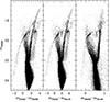 |
Fig. 1. CMD of NGC 1835 obtained from the WFC3 dataset in all the filter combinations. |
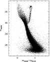 |
Fig. 2. CMD of the LMC field obtained from the ACS parallel observations. |
4. The horizontal branch of NGC 1835
The HB extension of NGC 1835 is fully appreciable in the CMDs involving the F300X filter, which has ‘guided’ the detection of hot stars (see Sect. 2). However, the peculiarity of this HB is not only its magnitude extension, but also its colour distribution: in fact, the HB appears to be well populated both in its red (0.5 < mF300X − mF606W < 0.8) and blue (−2.1 < mF300X − mF606W < 0.4) portions, and also shows a large population of stars in the instability strip.
4.1. The RR Lyrae population
The identification of RR Lyrae variable stars is a crucial step for the proper analysis of the HB morphology. For their identification we exploited a photometric ‘variability index’, defined as the ratio between the standard deviation of the star luminosities measured at different epochs (which provides an estimate of the amplitude of the light curve) and the internal photometric error (which provides an estimate of the quality of the star’s photometry; Kjeldsen & Frandsen 1992). For stars having magnitude values from different exposures that consistently fall within the photometric error, the variability index tends to approach unity. Conversely, an increase in the index value corresponds to an increasing probability of stellar variability. In the case of NGC 1835, we find that the variability indexes computed in the near-UV tend to be larger than those obtained in the optical bands, thus suggesting that the F300X filter is best suited for this kind of study. We therefore assumed as variable stars all the sources with a variability index higher than 2 in this filter.
The number of variable stars recovered with this approach is 95. However, since our dataset was not originally intended for variability studies, we complemented this information with the Optical Gravitational Lensing Experiment (OGLE) IV catalogue1, which provides information on variable stars and transient objects in the Magellanic Clouds and Galactic bulge. This catalogue presents an updated list of variables found in the direction of the cluster NGC 1835, for a total of 125 objects, mainly RR Lyrae (Soszyński et al. 2016). After proper cross-correlation, we found a total of 67 variable stars in the region of the instability strip in common between our catalogue and the OGLE one. Interestingly enough, 43 of them were also identified via the variability index, while the remaining 24 OGLE variables were possibly caught in low luminosity variation phases by our observations. In addition, the DAOPHOT variability index indicates that in the field of view sampled by our observations there are 52 more candidate RR Lyrae that are not included in the OGLE catalogue. Thus, NGC 1835 hosts a very large population of RR Lyrae variables, counting 119 objects in the field of view sampled by our observations: 67 are confirmed OGLE variables, and 52 are possible new candidates identified by the variability index (see Fig. 3).
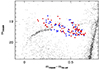 |
Fig. 3. CMD of NGC 1835, zoomed into the HB region. The 67 confirmed OGLE variables and 52 new candidate RR Lyrae are highlighted as red and blue circles, respectively. Only non-variable stars observed at r < 60″ from the centre are shown for reference, as black dots. |
4.2. Field decontamination and extension of the HB
As shown in Fig. 1, the main LMC field contamination along the HB is in the red portion of the branch, in the colour range 0 < mF300X − mF606W < 1.2, with a minor contribution in the adjacent colour bin 1.2 < mF300X − mF606W < 2 (‘extremely red’ portion). With the available datasets (only HST Wide Field and Planetary Camera 2 (WFPC2) images of the cluster are present in the HST archive), the decontamination through proper motions is not feasible. In fact, given the large distance of the LMC (Harris & Zaritsky 2009; Pietrzyński et al. 2019), a first epoch dataset with an astrometric quality better than that provided by the archive WFPC2 observations is required, possibly combined with a significantly longer time baseline between the two epochs. Thus, we performed a statistical decontamination of these portions of the HB taking advantage of the parallel ACS observations (Ferraro et al. 2019; Dalessandro et al. 2019). Schematically, after removing all the confirmed and candidate variables, we selected the HB stars in the (mF606W, mF300X − mF606W) CMD. Then, we used the position of these stars in the (mF606W, mF606W − mF814W) CMD to draw the optical selection boxes of the red and extremely red HB portions. We counted the number of stars belonging to ACS catalogue that fall within the two selection boxes and, dividing by the area sampled by the parallel observations, we finally obtained the density of LMC field stars contaminating the red and the extremely red portions of the HB. This procedure yielded a field density contamination of 17.28 and 3.44 stars per square arcminute, which corresponds to a total of 120 and 25 field stars potentially contaminating the red and the extremely red HB portions, respectively. The statistical decontamination was then performed taking into account the distance from the cluster centre and the geometric distance of each stars from the mean ridge line of the HB, since the membership probability typically decreases if these distances increase. Hence, the cluster (WFC3) sample has been divided into concentric annuli, and the expected number of contaminating stars was determined in each radial annulus from the estimated field density and the bin area. Finally, the estimated number of field stars has been removed from the WFC3 sample starting from the objects located at larger geometric distances from the HB mean ridge line.
The HB of NGC 1835 obtained after statistical decontamination counts 602 non-variable stars and is plotted in Fig. 4. For the sake of clarity, we also explicitly mark the large extension in colour (∼4 mag) and in magnitude (∼4.6) of the branch. Indeed, even neglecting the faintest stars detected at mF606W ∼ 24.2, the extension in magnitude and colour is remarkable: this is the first time that such an extended HB has been detected in an extragalactic cluster.
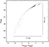 |
Fig. 4. HB of NGC 1835 after the statistical decontamination of the reddest portions. Only non-variable stars are plotted. The extension in colour (∼4 mag) and in magnitude (∼4.6 mag) is also marked. |
5. Reddening, distance modulus, and age of NGC 1835
For a more detailed description of the HB morphology of NGC 1835 we considered two Galactic GCs (namely, M 3 and M 13) as reference systems. These clusters have been extensively studied in the literature and their properties are well established (see Ferraro et al. 1997; Johnson et al. 2005; Sneden et al. 2004; Dalessandro et al. 2013; Cadelano et al. 2019, 2020a). They are two ‘twin’ GCs, with similar age, metallicity, and central density. They respectively have ages of 12.50 ± 0.50 Gyr and 13.00 ± 0.50 Gyr (Dotter et al. 2010), [Fe/H] = −1.50 ± 0.05 and [Fe/H] = −1.58 ± 0.04 (Carretta et al. 2009), and V-band central surface brightness μ0 = 16.64 mag arcsec−2 and 16.59 mag arcsec−2 (Harris 1996). In addition, they have a similar mass of about log M/M⊙ ∼ 5.8 (McLaughlin & van der Marel 2006; Pryor & Meylan 1993). These values are compatible with those measured in NGC 1835: [Fe/H] = −1.69 ± 0.01 (Mucciarelli et al. 2021), μ0 = 16.64 mag arcsec−2 in the F555W filter (Mackey & Gilmore 2003) and log M/M⊙ ∼ 5.83 (Mackey & Gilmore 2003). As for the age, there is general agreement on the fact that NGC 1835 belongs to the class of old LMC clusters, but the absolute age is still quite uncertain and strongly overestimated:  , corresponding to an age t ∼ 16 Gyr (see Olsen et al. 1998; Olszewski et al. 1991). In addition, the HB of M 13 shows a well extended and populated blue tail, reminiscent of that discovered in NGC 1835, but very few RR Lyrae (only ten are quoted in the Clement catalogue; Clement et al. 20012) and just a few stars redder than the instability strip. Conversely, M 3 hosts a large population of RR Lyrae (more than 200), similarly to NGC 1835, but no evidence of the blue tail. Hence, M 3 and M 13 are excellent reference clusters for an in-depth study of NGC 1835. Indeed, through the direct comparison of the CMDs we determined the reddening and the distance of NGC 1835, which are then used to estimate the age of the cluster. With this information in hand, we finally proceeded to a direct comparison between the HBs of the three systems, as well as the determination of the effective temperature distribution of the HB stars in NGC 1835 (Sect. 6).
We performed the cluster-to-cluster comparison in the optical (mF606W, mF606W − mF814W) CMD. To maximize the accuracy of such a comparison, we first constructed a field-decontaminated CMD of NGC 1835. We decided to perform a statistical decontamination following the prescriptions described in Giusti et al. (2023) and briefly summarized below. We considered an annular region of the CMD included between 5″ and 26″ from the cluster centre. The very central region has been excluded because it is typically sampled with larger photometric errors, and the most external one is rejected to keep low the number of contaminating field stars. Then, a region with the same area has been selected in the ACS catalogue of the LMC field and, for each star of this sample, we removed one star from the cluster sample according to its position in the CMD. In particular, we flagged as the most likely interloper (and removed it from the cluster sample) the closest star (in terms of magnitude and colour) to the considered star in the LMC field sample. The procedure was repeated several times considering different LMC field regions, finding qualitatively consistent results in all the cases.
The field-decontaminated CMD of NGC 1835 thus obtained was then compared with those of the two reference clusters, M 3 and M 13, by using the data collected in the ACS Survey of Galactic Globular Clusters (Anderson et al. 2008). We then aligned these CMDs with that of NGC 1835 by applying appropriate shifts in magnitude and colour, chosen on the basis of χ2 tests: for M 3 we used Δmag = 3.78 and Δcol = 0.07; for M 13 we applied Δmag = 4.37 and Δcol = 0.06. The left panel of Fig. 5 presents the comparison between the decontaminated CMD of NGC 1835 (black dots) and the CMD of M 3 (red dots). The right panel shows the same, but for M 13. Most of the evolutionary sequences of NGC 1835, such as the MS and the RGB, exhibit striking similarities with those of M 3 and M 13. Specifically, all the three clusters show a comparable morphology of the MS-TO region and have a similar colour extensions of the sub-giant branch. Moreover, the RGBs of the three clusters display comparable extensions and slopes. These results are consistent with the three clusters having similar ages and metallicities, as discussed above.
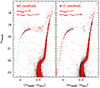 |
Fig. 5. Comparison between the decontaminated CMD of NGC 1835 (black dots) and the CMDs of M 3 and M 13 (red dots in the left and right panels, respectively) shifted to match that of NGC 1835. |
Using the extinction coefficients RF606W = 2.8192 and RF814W = 1.8552 (Cardelli et al. 1989; O’Donnell 1994) and assuming for M 3 a distance modulus of (m − M)0 = 15.00 ± 0.04 (Ferraro et al. 1999b; Dalessandro et al. 2013) and a colour excess E(B − V) = 0.01 (Ferraro et al. 1999b), we found (m − M)0 = 18.58 and E(B − V) = 0.08 for NGC 1835. The same results are obtained by adopting M 13 as a reference and thus assuming its distance modulus and reddening, (m − M)0 = 14.38 ± 0.05 and E(B − V) = 0.02 (Ferraro et al. 1999b). These findings are fully consistent with previous estimates in the literature: in fact, a reddening value of E(B − V) = 0.08 ± 0.02 and a distance modulus ranging between 18.43 ± 0.12 and 18.65 ± 0.16 are quoted in Olsen et al. (1998).
To determine the absolute age of NGC 1835 we adopted the isochrone fitting technique. This consists in comparing the cluster CMD with a set of isochrones of different ages to identify the one that best reproduces the observed evolutionary sequences. We extracted isochrones from two different databases, BaSTI (Pietrinferni et al. 2021) and PARSEC (Bressan et al. 2012; Chen et al. 2015). BaSTI isochrones have been computed for [Fe/H] = −1.7, an α-element abundance [α/Fe]= + 0.4 (Mucciarelli et al. 2021), and a standard helium abundance Y = 0.248. Similarly, we downloaded solar-scaled PARSEC isochrones with a total metallicity [M/H] = −1.4, which corresponds to [α/Fe]= + 0.4 and [Fe/H] = −1.7. Both datasets were downloaded for a suitable range of ages (between 10 Gyr and 15 Gyr in steps of 0.5 Gyr). They have been superposed to the observed CMD by adopting the distance modulus and the reddening values estimated above. A small colour offset of δ(mF606W − mF814W) = 0.015 mag (lower than the typical errors introduced by the photometric calibration) was applied to the isochrone in order to better match the data. Using χ2 tests, we compared the isochrones and the observed data in the most age-sensitive region of the CMD (namely, the MS-TO and the sub-giant branch, in a magnitude range 21.8 < mF606W < 23.0). For a maximum photometric quality of the data and to avoid severe contamination from the LMC field, we limited the analysis to an annular region between 15″ and 26″ from the cluster centre.
The results obtained for the two considered models are shown in Fig. 6. The left panels depict the trend of the χ2 values for different ages and show that, for both the adopted model, the minimum χ2 value (i.e., the best-fit solution) is found at an age of 12.5 Gyr, with a conservative uncertainty of ±1 Gyr. The right panels of Fig. 6 show the isochrones corresponding to the best-fit ages (solid red line) along with the uncertainty ranges (dashed lines).
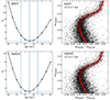 |
Fig. 6. Determination of NGC 1835 absolute age. Left panels: trend of the χ2 values obtained from the isochrone fitting of the MS-TO region of the models (top and bottom panels, respectively) computed for [Fe/H] = −1.7, [α/Fe]= + 0.4, Y = 0.248, and ages ranging between 10 Gyr and 15 Gyr. Right panels: decontaminated CMD of NGC 1835 with the BaSTI and PARSEC isochrones superposed (top and bottom panels, respectively), corresponding to the best-fit age (12.5 Gyr, solid lines) and the estimated age interval (±1 Gyr, dashed lines). |
6. The surprising HB morphology of NGC 1835
As mentioned above, the HB of M 13 shows a well extended and populated blue tail, very few RR Lyrae, and the portion redder than the instability strip that is poorly populated. Conversely, in M 3 the star distribution is peaked around the instability strip, with a large population of RR Lyrae, and the red and the blue side of the strip are both well populated, but with no evidence of a blue tail. These characteristics make the two Galactic GCs particularly useful for the description of the HB morphology in NGC 1835.
As shown in Fig. 4, the colours using the F300X filter tend to stretch the high-temperature tail of the branch, while compressing the low-temperature portion. Thus, better insights into the star distribution in the red (cold) side of the HB are obtainable in the purely optical colour (mF606W − mF814W), which also allows a clear identification of the location of the instability strip. Figure 7 shows the comparison in the optical CMD among the low-temperature portion of the HB observed in NGC 1835 (top panel), in M 3 (central panel) and in M 13 (bottom panel). The CMDs of M 3 and M 13 have been shifted to the distance and reddening of NGC 1835 estimated above. The similarity between M 3 and NGC 1835 in the morphology of this portion of the HB is impressive, and it is further supported by the existence of large populations of RR Lyrae detected in both systems. On the other hand, it is evident that the HB in M 13 extends mainly on the blue side of the instability strip, consistently with the low number of confirmed variables in this cluster.
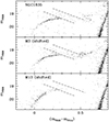 |
Fig. 7. Low-temperature portion of the HB of NGC 1835 (top panel) compared with those of M 3 (central panel) and M 13 (bottom panel). The CMD of M 3 and M 13 have been shifted to the same distance and reddening of NGC 1835. In all panels, the two dashed lines delimitate the region where most of the RR Lyrae observed at random phases are expected to be located. |
For the sake of comparison, Fig. 8 shows instead the comparison between the HB of NGC 1835 (left panel) and that of M 13 (right panel) in the optical/near-UV hybrid CMD. As usual the CMD of M 13 has been shifted to the distance of NGC 1835 estimated above. Only non-variable stars are plotted here. Although the filters used in this comparison are not exactly the same, the overall magnitude extension of the branch is strikingly similar. Notably, the colour extension in NGC 1835 looks wider than in M 13, with several stars reaching redder colours at the right-end side of the instability strip, where almost no objects are observed in M 13 (see also Fig. 7). This comparison therefore shows that the HB observed in NGC 1835 looks like a combination of the HBs of M 3 and M 13, with a well-populated red portion characterized by a relevant number of RR Lyrae (like in M 3, and at odds with M 13) and an extended blue tail (at odds with M 3, but as in M 13).
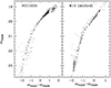 |
Fig. 8. HB of NGC 1835 (left panel) compared to that of M 13 (right panel). Variable stars are not shown. |
As last piece of information, we determined the temperature distribution of the HB stars in NGC 1835. In doing this, we first translated the decontaminated HB into the absolute plane, adopting the distance modulus and the reddening determined in Sect. 5. We then projected the non-variable stars perpendicularly onto the mean ridge line of the branch (see the inset in Fig. 9), thus obtaining their projected intrinsic colour and absolute magnitude. Then, to transform the (MF300X − MF606W) colour into effective temperature (Teff), we adopted the colour–temperature relation for zero-age HB models of appropriate metallicity ([Fe/H] = −1.7) extracted from the BASTI dataset (Pietrinferni et al. 2021). To complete the overall picture, we arbitrarily attributed Teff values to all the confirmed and candidates RR Lyrae in the temperature range covered by the instability strip (6000 < Teff < 7000). The resulting Teff distribution (see Fig. 9) shows a main peak in the red portion of the HB (possibly in the instability strip), and a long tail extending to temperatures as large as 30 000 K. The tail is not uniformly populated (in agreement with what observed in all other similar cases; see e.g., the discussion in Ferraro et al. 1998), but it seems to show a secondary peak (by far less populated than the main one) in the region between 15 000 and 20 000 K.
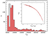 |
Fig. 9. Effective temperature distribution of the HB stars in NGC 1835. The histogram shaded in grey refers to the sample of 119 confirmed and candidate variable stars distributed within the range of temperatures covered by the instability strip (6000 < Teff < 7000). The inset shows the locations of non-variable HB stars in the absolute CMD (black dots) and the corresponding positions projected onto the HB mean ridge line (red dots along the solid black line). The colour axis is inverted (with bluer colours to the right) to be consistent with the x-axis of the histogram (increasing temperature to the right). |
7. Summary and conclusions
In the framework of a project aimed at performing a new characterization of the oldest and most compact stellar systems in the LMC, we have presented a detailed multi-wavelength photometric study of the GC NGC 1835. A set of near-UV and optical high-resolution images have been secured using the HST/WFC3. These images already revealed the presence of the small stellar system KMK 88-10 at just 2′ from the centre of NGC 1835, suggesting the exciting possibility that it has been captured by the close massive GC and is on the verge of tidal disruption (Giusti et al. 2023). In a companion paper (Giusti et al., in prep.), we will present the determination of the density profile and the structural parameters of NGC 1835, as well as its dynamical age measured from the sedimentation level of blue straggler stars following the dynamical clock prescription (Ferraro et al. 2018, 2020, 2023).
The present work has been devoted to the discussion of the HB morphology of NGC 1835, supported by new estimates of its distance, reddening, and age. In agreement with previous studies in the literature, we find a distance modulus (m − M)0 = 18.58 (corresponding to 52 kpc) and a colour excess E(B − V) = 0.08. The major result of the present investigation is the detection of an unexpected feature: despite all previous photometric studies (e.g., Olsen et al. 1998), our analysis, thanks to the use of a near-UV filter, has revealed the presence of a very extended blue tail of the HB. So far, such a feature has only been observed in a few cases in our Galaxy, namely in the so-called extreme blue tailed clusters, such as M 13, NGC 6752, NGC 2808, NGC 2419, and M80 (see Ferraro et al. 1997, 1998; Dalessandro et al. 2011, 2013; Onorato et al. 2023).
We have presented a detailed characterization of the observational properties of the HB: (i) the optical/near-UV CMDs reveal the presence of a pronounced blue tail extending well below the MS-TO: its extension is as large as 4.5 mag in both the near-UV and optical bands; (ii) the overall colour extension of the HB is also impressive, ranging from (mF300X − mF606W)∼ − 2.5 up to (mF300X − mF606W)∼2, thus covering a wide interval of effective temperatures, from 5000 up to 30 000 K; (iii) a large population of RR Lyrae (67 are confirmed by OGLE and 52 are new candidates) has been identified; and (iv) a comparison with two Milky Way GCs used as references has revealed that the HB of NGC 1835 seems to be a combination of the HBs of the ‘classical twin GCs’ M 3 and M 13, simultaneously showing the main properties of both their morphologies: a rich population of HB stars on both sides of the instability strip and a large sample of variable stars (as in M 3), combined with an extended blue tail (as observed in M 13). The striking similarity with the HB morphology of M 13 suggests that NGC 1835 should also harbour a population of slowly cooling white dwarfs (see Chen et al. 2021). Unfortunately, however, their detection is beyond the photometric capacity of the current generation of instruments.
The HB evolutionary stage is characterized by helium combustion in the stellar core and hydrogen burning in an adjacent shell. The different colour (temperature) distributions of HB stars (i.e., the different HB morphologies) observed in old stellar systems are a manifestation of the different mass distributions of the stars that reach this evolutionary stage. More specifically, since in old stellar systems such as NGC 1835 (for which we have estimated an age of 12.5 ± 1 Gyr; see Sect. 5) the core mass of all HB stars is essentially set by the occurrence of the helium flash, the key parameter responsible for the HB morphology is the residual mass of the envelope, with stars with high envelope masses in red regions along the HB (i.e., at low effective temperatures) and stars with low envelope masses in blue regions (i.e., at high Teff). One of the most obvious parameters that can impact the mass of the residual envelope (and hence the distribution in colour) is the mass loss occurring along the RGB (see Origlia et al. 2002, 2007, 2014). However, age spreads and helium abundance differences (possibly related to the light-element multiple population phenomenon; e.g., Milone et al. 2014) also affect the mass of stars that reach the HB phase. Hence, understanding the origin of the HB morphology, which depends on many different parameters, is a complex task (see e.g., Catelan 2009; Gratton et al. 2010; Milone et al. 2014). While a spread of stellar ages is excluded in NGC 1835 by the apparent narrowness of its MS-TO (see Sect. 5), the combined action of mass loss and helium spread (see e.g., Tailo et al. 2020) can in principle account for its complex HB morphology. Indeed, Dalessandro et al. (2013) discuss the HB morphology of M 3 and M 13, concluding that it can be interpreted in terms of different helium contents. Unfortunately, the photometric band combination used here is not optimized for detecting light-element multiple populations and, in fact, we observe no evidence of splitting or broadening along the evolutionary sequences in the CMD. A forthcoming paper will be devoted to a detailed reconstruction of the observed HB morphology through appropriate population synthesis, following an approach similar to that discussed in the cases of NGC 1904 and M 13 by Dalessandro et al. (2013).
Acknowledgments
This work is part of the project Cosmic-Lab at the Physics and Astronomy Department “A. Righi” of the Bologna University (http://www.cosmic-lab.eu/Cosmic-Lab/Home.html).
References
- Anderson, J., Sarajedini, A., Bedin, L. R., et al. 2008, AJ, 135, 2055 [Google Scholar]
- Baumgardt, H., Parmentier, G., Anders, P., et al. 2013, MNRAS, 430, 676 [NASA ADS] [CrossRef] [Google Scholar]
- Bellini, A., Anderson, J., & Bedin, L. R. 2011, PASP, 123, 622 [CrossRef] [Google Scholar]
- Bressan, A., Marigo, P., Girardi, L., et al. 2012, MNRAS, 427, 127 [NASA ADS] [CrossRef] [Google Scholar]
- Brocato, E., Castellani, V., Ferraro, F. R., et al. 1996, MNRAS, 282, 614 [NASA ADS] [CrossRef] [Google Scholar]
- Brown, T. M. 2004, Ap&SS, 291, 215 [NASA ADS] [CrossRef] [Google Scholar]
- Cadelano, M., Ferraro, F. R., Istrate, A. G., et al. 2019, ApJ, 875, 25 [NASA ADS] [CrossRef] [Google Scholar]
- Cadelano, M., Chen, J., Pallanca, C., et al. 2020a, ApJ, 905, 63 [NASA ADS] [CrossRef] [Google Scholar]
- Cadelano, M., Dalessandro, E., Webb, J. J., et al. 2020b, MNRAS, 499, 2390 [NASA ADS] [CrossRef] [Google Scholar]
- Cadelano, M., Saracino, S., Dalessandro, E., et al. 2020c, ApJ, 895, 54 [NASA ADS] [CrossRef] [Google Scholar]
- Cadelano, M., Dalessandro, E., Salaris, M., et al. 2022a, ApJ, 924, L2 [NASA ADS] [CrossRef] [Google Scholar]
- Cadelano, M., Ferraro, F. R., Dalessandro, E., et al. 2022b, ApJ, 941, 69 [CrossRef] [Google Scholar]
- Cardelli, J. A., Clayton, G. C., & Mathis, J. S. 1989, Interstellar Dust, 135, 5 [NASA ADS] [Google Scholar]
- Carretta, E., Bragaglia, A., Gratton, R., et al. 2009, A&A, 508, 695 [NASA ADS] [CrossRef] [EDP Sciences] [Google Scholar]
- Catelan, M. 2009, Ap&SS, 320, 261 [Google Scholar]
- Chen, J., Ferraro, F. R., Cadelano, M., et al. 2021, Nat. Astron., 5, 1170 [NASA ADS] [CrossRef] [Google Scholar]
- Chen, J., Ferraro, F. R., Cadelano, M., et al. 2022, ApJ, 934, 93 [NASA ADS] [CrossRef] [Google Scholar]
- Chen, J., Ferraro, F. R., Salaris, M., et al. 2023a, ApJ, 950, 155 [CrossRef] [Google Scholar]
- Chen, J., Cadelano, M., Pallanca, C., et al. 2023b, ApJ, 948, 84 [NASA ADS] [CrossRef] [Google Scholar]
- Chen, Y., Bressan, A., Girardi, L., et al. 2015, MNRAS, 452, 1068 [Google Scholar]
- Clement, C. M., Muzzin, A., Dufton, Q., et al. 2001, AJ, 122, 2587 [NASA ADS] [CrossRef] [Google Scholar]
- Dalessandro, E., Salaris, M., Ferraro, F. R., et al. 2011, MNRAS, 410, 694 [NASA ADS] [CrossRef] [Google Scholar]
- Dalessandro, E., Schiavon, R. P., Rood, R. T., et al. 2012, AJ, 144, 126 [NASA ADS] [CrossRef] [Google Scholar]
- Dalessandro, E., Salaris, M., Ferraro, F. R., et al. 2013, MNRAS, 430, 459 [NASA ADS] [CrossRef] [Google Scholar]
- Dalessandro, E., Ferraro, F. R., Bastian, N., et al. 2019, A&A, 621, A45 [NASA ADS] [CrossRef] [EDP Sciences] [Google Scholar]
- Deras, D., Cadelano, M., Ferraro, F. R., et al. 2023, ApJ, 942, 104 [CrossRef] [Google Scholar]
- Deras, D., Cadelano, M., Lanzoni, B., et al. 2024, A&A, 681, A38 [NASA ADS] [CrossRef] [EDP Sciences] [Google Scholar]
- Dorman, B., Rood, R. T., & O’Connell, R. W. 1993, ApJ, 419, 596 [NASA ADS] [CrossRef] [Google Scholar]
- Dorman, B., O’Connell, R. W., & Rood, R. T. 1995, ApJ, 442, 105 [NASA ADS] [CrossRef] [Google Scholar]
- Dotter, A., Sarajedini, A., Anderson, J., et al. 2010, ApJ, 708, 698 [Google Scholar]
- Erkal, D., Belokurov, V., Laporte, C. F. P., et al. 2019, MNRAS, 487, 2685 [Google Scholar]
- Ferraro, F. R., Fusi Pecci, F., Testa, V., et al. 1995, MNRAS, 272, 391 [NASA ADS] [CrossRef] [Google Scholar]
- Ferraro, F. R., Paltrinieri, B., Fusi Pecci, F., et al. 1997, ApJ, 484, L145 [Google Scholar]
- Ferraro, F. R., Paltrinieri, B., Fusi Pecci, F., et al. 1998, ApJ, 500, 311 [NASA ADS] [CrossRef] [Google Scholar]
- Ferraro, F. R., Paltrinieri, B., Rood, R. T., et al. 1999a, ApJ, 522, 983 [CrossRef] [Google Scholar]
- Ferraro, F. R., Messineo, M., Fusi Pecci, F., et al. 1999b, AJ, 118, 1738 [NASA ADS] [CrossRef] [Google Scholar]
- Ferraro, F. R., D’Amico, N., Possenti, A., et al. 2001, ApJ, 561, 337 [NASA ADS] [CrossRef] [Google Scholar]
- Ferraro, F. R., Sills, A., Rood, R. T., et al. 2003, ApJ, 588, 464 [NASA ADS] [CrossRef] [Google Scholar]
- Ferraro, F. R., Origlia, L., Testa, V., et al. 2004, ApJ, 608, 772 [NASA ADS] [CrossRef] [Google Scholar]
- Ferraro, F. R., Mucciarelli, A., Carretta, E., et al. 2006, ApJ, 645, L33 [NASA ADS] [CrossRef] [Google Scholar]
- Ferraro, F. R., Lanzoni, B., Dalessandro, E., et al. 2012, Nature, 492, 393 [Google Scholar]
- Ferraro, F. R., Lanzoni, B., Raso, S., et al. 2018, ApJ, 860, 36 [NASA ADS] [CrossRef] [Google Scholar]
- Ferraro, F. R., Lanzoni, B., Dalessandro, E., et al. 2019, Nat. Astron., 3, 1149 [NASA ADS] [CrossRef] [Google Scholar]
- Ferraro, F. R., Lanzoni, B., & Dalessandro, E. 2020, Rendiconti Lincei. Scienze Fisiche e Naturali, 31, 19 [NASA ADS] [CrossRef] [Google Scholar]
- Ferraro, F. R., Lanzoni, B., Vesperini, E., et al. 2023, ApJ, 950, 145 [NASA ADS] [CrossRef] [Google Scholar]
- Gaia Collaboration (Vallenari, A., et al.) 2023, A&A, 674, A1 [NASA ADS] [CrossRef] [EDP Sciences] [Google Scholar]
- Giusti, C., Cadelano, M., Ferraro, F. R., et al. 2023, ApJ, 953, 125 [CrossRef] [Google Scholar]
- Glatt, K., Grebel, E. K., & Koch, A. 2010, A&A, 517, A50 [CrossRef] [EDP Sciences] [Google Scholar]
- Gratton, R. G., Carretta, E., Bragaglia, A., et al. 2010, A&A, 517, A81 [CrossRef] [EDP Sciences] [Google Scholar]
- Greggio, L., & Renzini, A. 1990, ApJ, 364, 35 [Google Scholar]
- Harris, W. E. 1996, VizieR Online Data Catalog: VII/195 [Google Scholar]
- Harris, J., & Zaritsky, D. 2009, AJ, 138, 1243 [NASA ADS] [CrossRef] [Google Scholar]
- Hill, V., Franois, P., Spite, M., Primas, F., & Spite, F. 2000, A&A, 364, L19 [NASA ADS] [Google Scholar]
- Johnson, C. I., Kraft, R. P., Pilachowski, C. A., et al. 2005, PASP, 117, 1308 [CrossRef] [Google Scholar]
- Kjeldsen, H., & Frandsen, S. 1992, PASP, 104, 413 [NASA ADS] [CrossRef] [Google Scholar]
- Lanzoni, B., Dalessandro, E., Ferraro, F. R., et al. 2007, ApJ, 663, 267 [NASA ADS] [CrossRef] [Google Scholar]
- Lanzoni, B., Ferraro, F. R., Alessandrini, E., et al. 2016, ApJ, 833, L29 [NASA ADS] [CrossRef] [Google Scholar]
- Lanzoni, B., Ferraro, F. R., Dalessandro, E., et al. 2019, ApJ, 887, 176 [NASA ADS] [CrossRef] [Google Scholar]
- Lee, H. C., Lee, Y.-W., & Gibson, B. K. 2002, AJ, 124, 2664 [CrossRef] [Google Scholar]
- Mackey, A. D., & Gilmore, G. F. 2003, MNRAS, 340, 175 [Google Scholar]
- Maraston, C. 2005, MNRAS, 362, 799 [NASA ADS] [CrossRef] [Google Scholar]
- McLaughlin, D. E., & van der Marel, R. P. 2006, VizieR Online Data Catalog: J/ApJS/161/304 [Google Scholar]
- Meurer, G. R., Lindler, D. J., Blakeslee, J., et al. 2003, Proc. SPIE, 4854, 507 [NASA ADS] [CrossRef] [Google Scholar]
- Milone, A. P., Marino, A. F., Dotter, A., et al. 2014, ApJ, 785, 21 [NASA ADS] [CrossRef] [Google Scholar]
- Mucciarelli, A., Origlia, L., Ferraro, F. R., et al. 2006, ApJ, 646, 939 [NASA ADS] [CrossRef] [Google Scholar]
- Mucciarelli, A., Origlia, L., & Ferraro, F. R. 2010, ApJ, 717, 277 [NASA ADS] [CrossRef] [Google Scholar]
- Mucciarelli, A., Massari, D., Minelli, A., et al. 2021, Nat. Astron., 5, 1247 [NASA ADS] [CrossRef] [Google Scholar]
- O’Donnell, J. E. 1994, ApJ, 422, 158 [Google Scholar]
- Olsen, K. A. G., Hodge, P. W., Mateo, M., et al. 1998, MNRAS, 300, 665 [NASA ADS] [CrossRef] [Google Scholar]
- Olszewski, E. W., Schommer, R. A., Suntzeff, N. B., et al. 1991, AJ, 101, 515 [NASA ADS] [CrossRef] [Google Scholar]
- Olszewski, E. W., Suntzeff, N. B., & Mateo, M. 1996, ARA&A, 34, 511 [NASA ADS] [CrossRef] [Google Scholar]
- Onorato, S., Cadelano, M., Dalessandro, E., et al. 2023, A&A, 677, A8 [NASA ADS] [CrossRef] [EDP Sciences] [Google Scholar]
- Origlia, L., Ferraro, F. R., Fusi Pecci, F., et al. 2002, ApJ, 571, 458 [NASA ADS] [CrossRef] [Google Scholar]
- Origlia, L., Rood, R. T., Fabbri, S., et al. 2007, ApJ, 667, L85 [NASA ADS] [CrossRef] [Google Scholar]
- Origlia, L., Ferraro, F. R., Fabbri, S., et al. 2014, A&A, 564, A136 [NASA ADS] [CrossRef] [EDP Sciences] [Google Scholar]
- Percival, S. M., & Salaris, M. 2011, MNRAS, 412, 244 [Google Scholar]
- Pietrinferni, A., Hidalgo, S., Cassisi, S., et al. 2021, ApJ, 908, 102 [NASA ADS] [CrossRef] [Google Scholar]
- Pietrzynski, G., & Udalski, A. 2000, Acta Astron., 50, 337 [NASA ADS] [Google Scholar]
- Pietrzyński, G., Graczyk, D., Gallenne, A., et al. 2019, Nature, 567, 200 [Google Scholar]
- Pryor, C., & Meylan, G. 1993, Structure and Dynamics of Globular Clusters, 50, 357 [NASA ADS] [Google Scholar]
- Raso, S., Ferraro, F. R., Dalessandro, E., et al. 2017, ApJ, 839, 64 [NASA ADS] [CrossRef] [Google Scholar]
- Schiavon, R. P., Rose, J. A., Courteau, S., et al. 2004, ApJ, 608, L33 [NASA ADS] [CrossRef] [Google Scholar]
- Sneden, C., Kraft, R. P., Guhathakurta, P., et al. 2004, AJ, 127, 2162 [NASA ADS] [CrossRef] [Google Scholar]
- Soszyński, I., Udalski, A., Szymański, M. K., et al. 2016, Acta Astron., 66, 131 [NASA ADS] [Google Scholar]
- Stetson, P. B. 1987, PASP, 99, 191 [Google Scholar]
- Stetson, P. B. 1994, PASP, 106, 250 [Google Scholar]
- Tailo, M., Milone, A. P., Lagioia, E. P., et al. 2020, MNRAS, 498, 5745 [CrossRef] [Google Scholar]
All Figures
|
Fig. 1. CMD of NGC 1835 obtained from the WFC3 dataset in all the filter combinations. |
| In the text | |
|
Fig. 2. CMD of the LMC field obtained from the ACS parallel observations. |
| In the text | |
|
Fig. 3. CMD of NGC 1835, zoomed into the HB region. The 67 confirmed OGLE variables and 52 new candidate RR Lyrae are highlighted as red and blue circles, respectively. Only non-variable stars observed at r < 60″ from the centre are shown for reference, as black dots. |
| In the text | |
|
Fig. 4. HB of NGC 1835 after the statistical decontamination of the reddest portions. Only non-variable stars are plotted. The extension in colour (∼4 mag) and in magnitude (∼4.6 mag) is also marked. |
| In the text | |
|
Fig. 5. Comparison between the decontaminated CMD of NGC 1835 (black dots) and the CMDs of M 3 and M 13 (red dots in the left and right panels, respectively) shifted to match that of NGC 1835. |
| In the text | |
|
Fig. 6. Determination of NGC 1835 absolute age. Left panels: trend of the χ2 values obtained from the isochrone fitting of the MS-TO region of the models (top and bottom panels, respectively) computed for [Fe/H] = −1.7, [α/Fe]= + 0.4, Y = 0.248, and ages ranging between 10 Gyr and 15 Gyr. Right panels: decontaminated CMD of NGC 1835 with the BaSTI and PARSEC isochrones superposed (top and bottom panels, respectively), corresponding to the best-fit age (12.5 Gyr, solid lines) and the estimated age interval (±1 Gyr, dashed lines). |
| In the text | |
|
Fig. 7. Low-temperature portion of the HB of NGC 1835 (top panel) compared with those of M 3 (central panel) and M 13 (bottom panel). The CMD of M 3 and M 13 have been shifted to the same distance and reddening of NGC 1835. In all panels, the two dashed lines delimitate the region where most of the RR Lyrae observed at random phases are expected to be located. |
| In the text | |
|
Fig. 8. HB of NGC 1835 (left panel) compared to that of M 13 (right panel). Variable stars are not shown. |
| In the text | |
|
Fig. 9. Effective temperature distribution of the HB stars in NGC 1835. The histogram shaded in grey refers to the sample of 119 confirmed and candidate variable stars distributed within the range of temperatures covered by the instability strip (6000 < Teff < 7000). The inset shows the locations of non-variable HB stars in the absolute CMD (black dots) and the corresponding positions projected onto the HB mean ridge line (red dots along the solid black line). The colour axis is inverted (with bluer colours to the right) to be consistent with the x-axis of the histogram (increasing temperature to the right). |
| In the text | |
Current usage metrics show cumulative count of Article Views (full-text article views including HTML views, PDF and ePub downloads, according to the available data) and Abstracts Views on Vision4Press platform.
Data correspond to usage on the plateform after 2015. The current usage metrics is available 48-96 hours after online publication and is updated daily on week days.
Initial download of the metrics may take a while.