| Issue |
A&A
Volume 684, April 2024
|
|
|---|---|---|
| Article Number | L6 | |
| Number of page(s) | 8 | |
| Section | Letters to the Editor | |
| DOI | https://doi.org/10.1051/0004-6361/202348969 | |
| Published online | 08 April 2024 | |
Letter to the Editor
A too-many-dwarf-galaxy-satellites problem in the M 83 group
1
Institute of Physics, Laboratory of Astrophysics, Ecole Polytechnique Fédérale de Lausanne (EPFL), 1290 Sauverny, Switzerland
e-mail: oliver.muller@epfl.ch
2
Université de Strasbourg, CNRS, Observatoire astronomique de Strasbourg (ObAS), UMR 7550, 67000 Strasbourg, France
3
Leibniz-Institut fur Astrophysik Potsdam (AIP), An der Sternwarte 16, 14482 Potsdam, Germany
4
Space physics and Astronomy Research Unit, University of Oulu, Oulu 90014, Finland
5
European Southern Observatory, Karl-Schwarzschild Strasse 2, 85748 Garching, Germany
Received:
15
December
2023
Accepted:
13
March
2024
Dwarf galaxies in groups of galaxies provide excellent test cases for models of structure formation. This led to a so-called small-scale crisis, including the famous missing-satellites and too-big-to-fail problems. It was suggested that these two problems can be resolved by introducing baryonic physics to cosmological simulations. We tested the nearby grand spiral M 83 – a Milky Way sibling – to determine whether its number of dwarf galaxy companions is compatible with today’s Λ cold dark matter model using two methods: with cosmological simulations that include baryons and with theoretical predictions from the subhalo mass function. By employing distance measurements, we recovered a list of confirmed dwarf galaxies within 330 kpc of M 83 down to a magnitude of MV = −10. We find that both the state-of-the-art hydrodynamical cosmological simulation Illustris-TNG50 and theoretical predictions agree with the number of confirmed satellites around M 83 at the bright end of the luminosity function (> 108 solar masses) but underestimate it at the faint end (down to 106 solar masses) at more than 3σ and 5σ levels, respectively. This indicates a too-many-satellites problem for M 83 in the Λ cold dark matter model. The actual degree of tension with cosmological models is underestimated because the number of observed satellites is incomplete due to the high contamination of spurious stars and Galactic cirrus.
Key words: galaxies: dwarf / galaxies: groups: individual: M83 / galaxies: luminosity function / mass function
© The Authors 2024
 Open Access article, published by EDP Sciences, under the terms of the Creative Commons Attribution License (https://creativecommons.org/licenses/by/4.0), which permits unrestricted use, distribution, and reproduction in any medium, provided the original work is properly cited.
This article is published in open access under the Subscribe to Open model. Subscribe to A&A to support open access publication.
1. Introduction
In the past few years, the task of improving and extending the census of dwarf galaxies in the nearby universe has received an immense boost. This is thanks to the development and improvement of instruments and facilities (e.g., Abazajian et al. 2003; Meyer et al. 2004; Gwyn 2008; Bacon et al. 2010; Abraham & van Dokkum 2014; Miyazaki et al. 2018; Dey et al. 2019) as well as the general interest in these objects in the context of cosmology and galaxy formation (e.g., Kroupa et al. 2010; Crnojević et al. 2012; Duc et al. 2015; Weinberg et al. 2015; Bull et al. 2016; Bullock & Boylan-Kolchin 2017; Helmi et al. 2018; van Dokkum et al. 2018; Saifollahi et al. 2021; Pawlowski 2021; Sales et al. 2022; Kanehisa et al. 2023a; Müller et al. 2023). The dwarf galaxy abundance gives valuable insights into models of structure formation. The apparent discrepancies between the number of subhalos predicted by dark-matter-only cosmological simulations and the observed Milky Way satellites, namely the missing-satellite problem (Moore et al. 1999; Tollerud et al. 2008) and the too-big-to-fail problem (Boylan-Kolchin et al. 2011; Garrison-Kimmel et al. 2014), has pushed the community to improve our understanding of the role of baryons within galaxies (Simon & Geha 2007; Wetzel et al. 2016). Today, the observed luminosity function (LF) of the Milky Way and Andromeda satellites can be reproduced by cosmological simulations when baryonic effects such as supernova feedback are included (Sawala et al. 2016; Simpson et al. 2018; Revaz & Jablonka 2018). However, the question remains as to whether these results are valid outside of the Local Group, especially because the Local Group was used to calibrate the baryonic effects, making these successes not independent from the observations. Other problems, such as a tension in the motion and distribution of the satellites around the Milky Way and Andromeda, are still open to debate (Ibata et al. 2013; Libeskind et al. 2015; Pawlowski 2018, 2021; Sawala et al. 2023).
To see how typical our Local Group is, dwarf galaxies in other nearby groups need to be discovered and their memberships to the host galaxies have to be accurately established. This is a major undertaking. The membership determination requires the identification of small, low-surface-brightness galaxies and accurate distance measurements for them (Carlsten et al. 2022). However, getting this distance information is observationally expensive at the faint end of the LF, especially when there is a large number of dwarf galaxy candidates to follow up on (e.g., Chiboucas et al. 2009; Javanmardi et al. 2016; Müller et al. 2018a; Habas et al. 2020; Crosby et al. 2023). Using the tip of the red giant branch (TRGB; Da Costa & Armandroff 1990; Lee et al. 1993) as a standard candle, it takes one orbit per target for galaxies within < 10 Mpc with the Hubble Space Telescope (HST; e.g., Karachentsev et al. 2007; Chiboucas et al. 2013; Crnojević et al. 2019), or several hours of observation with ground-based 8-meter-class telescopes, such as the Very Large Telescope (VLT; see, e.g., Bird et al. 2015). Determining distances via the period–luminosity relations (Leavitt & Pickering 1912) of variable stars that can be used as distance indicators is more difficult due to the need for multi-epoch observations combined with the paucity (or absence) of young Cepheid variables and the faint magnitudes of RR Lyrae in dwarf galaxies. RR Lyrae in particular are only observable out to distances of about 2 Mpc with the HST (Da Costa et al. 2010). Type II Cepheids are brighter and can thus be observed to slightly larger distances in dwarf galaxies that host intermediate-age and old stellar populations. However, they are less numerous than RR Lyrae and have so far only been studied within the Local Group (Bhardwaj 2020). Beasley et al. (2024) recently suggested that the velocity dispersion of globular clusters is an excellent distance indicator, on par with the TRGB. Their independent measurement of the distance to Centaurus A (Cen A) is consistent with previous distance estimates based on other distance indicators. However, getting high-resolution spectroscopy for globular cluster systems is an expensive undertaking and may not always be feasible.
Another way to measure distances – which is currently only accurately applicable for early-type galaxies – is the surface brightness fluctuation (SBF) method (Tonry & Schneider 1988). While not as accurate as the TRGB method, it can be used on sufficiently deep images to estimate the distance and, with that, the membership of the dwarf galaxies to a potential host. With this technique, several of the dwarf galaxy candidates found around M 101 (Javanmardi et al. 2016; Müller et al. 2017b; Bennet et al. 2017) could either be confirmed or excluded (Carlsten et al. 2019b). Carlsten et al. (2022), exploiting public data, successfully extended this SBF analysis to other giant galaxies in the nearby universe, showing that the SBF method is a serious alternative for confirming or rejecting the membership of dwarf galaxies in group environments. However, we also note that when it comes to precise distance measurements, the SBF method may fail (see, e.g., Jerjen & Rejkuba 2001 for a direct comparison of the SBF and TRGB distance measurements of the same dwarf galaxy).
In terms of cosmological predictions, the abundance of dwarf galaxies in nearby groups has been addressed in a few recent studies. Around M 94 – a giant spiral galaxy at the heart of the Canes Venatici I cloud – an apparent lack of dwarf galaxy satellites was found (Smercina et al. 2018). Employing a deep imaging campaign with the Hyper Suprime Cam and resolving the upper part of the red giant branch, Smercina et al. (2018) surveyed the 150 kpc vicinity around M 94 and found only two satellites. Their membership was established via the TRGB method. This is in stark contrast to the expected number of satellites of five to ten, reviving the missing-satellite problem. On the other hand, for Cen A – a giant elliptical galaxy that has been the subject of several dedicated deep surveys (Crnojević et al. 2014, 2016, 2019; Müller et al. 2017a, 2019, 2021; Taylor et al. 2017, 2018) – the LF within 200 kpc of Cen A is compatible within 2σ with cosmological simulations that include baryonic physics (Müller et al. 2019). Similarly, for low-mass host galaxies in the local galactic neighborhood, as well as the high-redshift universe, the LF agrees well with cosmological predictions, when biases in observations are taken into account (Müller & Jerjen 2020; Roberts et al. 2021). Carlsten et al. (2021) used the stellar–halo mass relation to predict the number of satellites for 12 giant galaxies in the nearby universe (including Cen A and M 94) and compared it to observations. They found a large scatter in the LF, which is in agreement with cosmology, but pointed out that on the bright and faint ends there are more observed dwarfs than expected. Crosby et al. (2023) investigated the LF of NGC 2683 and other nearby giant galaxies with respect to the brightest dwarfs. Studying the magnitude gap between the host galaxy and the brightest satellite, they find that three out of six systems have a larger magnitude gap than expected from cosmological simulations (namely TNG100 of the Illustris suit of simulations; Springel et al. 2018), meaning that the brightest satellites may be missing.
These ambiguous results demonstrate the urgent need for complete dwarf galaxy samples within nearby galaxy groups to study the abundance of satellites. Here, we present a census of the spiral galaxy M 83 (NGC 5236) – also known as the Southern Pinwheel Galaxy – which is one of the closest neighbours to our Local Group. This late-type galaxy is at a distance of D ≃ 4.9 Mpc (Herrmann et al. 2008) and with Cen A at D ≃ 3.8 Mpc (Rejkuba 2004) forms the Centaurus group, which is similar to the Local Group. Several of Cen A’s satellite members are in projection closer to M 83; thus, there is a potential for confusion, which requires distance measurements to resolve. The mass of M 83 has been studied by different groups. Recently, the velocity of the flat part of the rotation curve (tracing its mass) was updated from vflat ≈ 150 km s−1 (Kamphuis et al. 2015) to vflat ≈ 190 km s−1 (Dykes et al. 2021). This is compatible with the rotation curve of the Milky Way, indicating that the two systems have similar masses and should therefore follow the same scaling relations when it comes to the number of expected dwarf galaxy satellites (Javanmardi et al. 2019).
2. Luminosity function of the M 83 group
The M83 group has 13 confirmed dwarf galaxies and eight unconfirmed dwarf galaxy candidates within a projected separation of 330 kpc (Müller et al. 2015). The most distant confirmed M 83 satellite – KK 195 – is at a projected distance of ≈330 kpc. Several dwarf galaxy candidates (Müller et al. 2015) are within this radius. These candidates are: dw1326-29, dw1329-32, dw1330-32, dw1334-32, dw1335-33, dw1336-32, dw1337-33, and dw1337-26 (Müller et al. 2015), as well as an additional dwarf galaxy candidate – dw1341-29 – that we serendipitously discovered while exploring the NOAO Science Archive. To determine the magnitude of dw1341-29, we fitted an exponential profile using Galfit. For all the unconfirmed dwarf galaxy candidates, we applied the SBF method to measure their distance and confirm or reject their memberships to M 83.
While in the NOAO Science Archive there is not a deep homogeneous dataset covering the whole 330 kpc, there are several pointings that we used to test whether we could determine a SBF signal for the dwarf candidates. In the following we discuss each candidate with respect to its potential SBF signal. The dwarf candidates dw1334-32 and dw1335-33 are too faint and have a too-low surface brightness to allow their SBF to be measured; therefore, we removed them from our confirmed dwarf galaxy list. However, they were already listed as unlikely candidates in Müller et al. (2015) and are likely false positives – neither are visible in deeper images from the Dark Energy Camera Legacy Survey (DECaLS; Dey et al. 2019), and dw1335-33 has a suspicious edge in the luminosity distribution in Fig. 2 of Müller et al. (2015) and may be an artifact coming from the stacking of the individual exposures. Each of the remaining candidates has combined exposure times ranging from 1310 to 28 285 s in g, r, or i. These stacked exposures are deep enough to test whether there is a SBF signal consistent with a membership to the M 83 group. To measure the SBF, we followed the steps suggested by Carlsten et al. (2019a). Only the dwarf galaxy candidate dw1341-29 shows a sign of being resolved. Its morphology and fluctuation signal resemble those of the two dwarf spheroidals dw1335-29 and dw1340-30 (see Fig. 1), which have been confirmed with HST and VLT observations (Carrillo et al. 2017; Müller et al. 2018b). This dwarf galaxy candidate must therefore be a nearby object. The dwarf galaxy candidate dw1337-26 looks to be part of a ring of scattered light and is therefore an artifact. The dwarf candidate dw1336-32 is part of a cirrus patch. The central part of this cirrus appears as a distinct, round feature, resembling the morphology of a dwarf galaxy. However, faint, adjacent cirrus patches stretching out toward the north and the southeast are clearly visible (see Fig. B.1). For the rest, we can confirm that there is no visible SBF signal, meaning that they are real objects but background galaxies that do not belong to Cen A or M 83. This is consistent with recent HI observations that covered the region around M 83 and shows that dw1328-29 – a previously listed dwarf galaxy candidate of M 83 (Müller et al. 2015) – is a background dwarf galaxy (For et al. 2019). All of these candidates, together with the two previously confirmed dwarf spheroidals, are shown in Fig. 1.
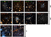 |
Fig. 1. Color-composite images of previous dwarf galaxy candidates of M 83 that have an optical counterpart in deeper images. The galaxies that feature an SBF are labeled in green and objects without any SBF signal in red. |
The previous assessment of a potential SBF signal leaves us with a census of 13 confirmed dwarf galaxies within 330 kpc of M 83 down to at least −10 mag. In Table A.1 we compile all confirmed dwarf galaxies of M 83, and in Fig. 2 we show their on-sky distribution. We further show their line-of-sight velocities, which are all within ±100 km s−1 of M 83’s velocity, which can serve as another means of establishing memberships to the group. Special attention is required for the tidally disrupted dwarf KK 208. This object is a stream with an estimated baryonic mass of 1.0 × 10⁸ M⊙ (Barnes et al. 2014), corresponding to a V-band magnitude of ≈−15.9. This puts it among the brightest satellites in M83. When comparing the M83 satellite system with simulations, we tested the results by including and excluding this system. We note that the results described in the next section do not change if we include or exclude KK 208.
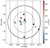 |
Fig. 2. Field around M 83. The large dot corresponds to M 83 and the small dots to confirmed dwarf galaxies. In color are dwarf galaxies with velocity measurements, in gray without. The thin circle corresponds to the virial radius of M 83 and the large circle to 330 kpc. |
3. Comparison to ΛCDM models
Next we compared the observed LF of the M 83 to the predicted number of satellites based on Λ cold dark matter (CDM) galaxy formation models using two different methods, that is, (a) using a state-of-the art hydrodynamical cosmological simulation and (b) using theoretical predictions from the subhalo mass function.
3.1. Illustris-TNG50
First we used the publicly available z = 0 galaxy catalogs (Nelson et al. 2019) from the TNG50-1 simulation of the Illustris-TNG project, a large-scale cosmological simulation that includes hydrodynamics. This run has a box size of 51.7 Mpc and a dark matter particle mass mDM = 4.5 × 10⁵ solar masses. For the comparison, we followed the same approach as for Cen A (Müller et al. 2019). Based on the flat part of the rotation curve of M 83, the baryonic Tully-Fisher relation (McGaugh 2005) yields a baryonic mass of 0.7 × 10¹¹ solar masses. We selected the halo primaries within a baryonic mass range of 0.6 × 10¹¹ ≤ M ≤ 1.0 × 10¹¹; this is slightly skewed toward higher masses, which will result in a larger number of identified subhalos in the simulation but allows us to get a statistically more significant sample. This mass range is also consistent with the estimation of the baryonic content estimated from the K-band luminosity (0.43 × 10¹¹ solar masses; Karachentsev et al. 2013) and HI content (0.24 × 10¹¹ solar masses; Huchtmeier & Bohnenstengel 1981) and includes the baryonic mass estimation of the Milky Way (Cautun et al. 2020). We excluded all hosts that have another galaxy of the same or higher mass within 700 kpc to avoid compact groups or cluster environments. This gives us 146 isolated M 83 analogs. We then mock-observed these analogs by putting them at a distance of 4.9 Mpc with a random orientation. We excluded all subhalos falling within 0.2 degrees of the center, the optical diameter of M 83, which would obfuscate any potential dwarf galaxy present in this region. We constructed satellite catalogs by selecting all subhalos within 330 kpc, which corresponds to the farthest projected M 83 satellite distance, and within a depth of 350 kpc along the line of sight. This latter value was chosen to correspond to the observed line-of-sight depth in our sample, corrected for the typical distance uncertainties, and ensures no overlap with the satellite system of another nearby host given our 700 kpc isolation criterion.
The results from our comparison of the LF to Illustris-TNG50 are shown in Fig. 3. For three of the analogs, we did not observe any satellite brighter than MV = −10 whatsoever. Another two have only one such satellite. Most of the simulated analogs have several satellite galaxies within the detection volume, but overall their number is lower than that of the confirmed observed satellite galaxies. When compared to the observations, this means that the number of predicted subhalos in the simulation is typically lower than the observed LF. However, there are still a few M 83 analogs at higher masses that have similar LFs at the bright end (MV < −15). In Fig. 3 we provide the percentage of analogs that have a higher abundance of satellites in the simulation than observed, given at the luminosity steps of every observed satellite. At the bright end, the observed and expected LFs agree well, within 1σ. However, this quickly changes at the faint end. The discrepancy is largest between MV = −14 mag and MV = −12 mag, where it is in tension with the simulated analogs by over 3σ. This is intriguing because the observed LF is based on a shallow dwarf galaxy survey (Müller et al. 2015), meaning that the abundance of dwarf galaxies in this part of the LF is likely underestimated – some dwarf galaxies around M 83 may be hidden. Müller et al. (2015) injected artificial galaxies into the survey data and found that even at the bright end of the LF, only 80 percent of the artificial galaxies were rediscovered. This is due to the high density of stars and contamination of Galactic cirrus patches, making the detection of potential dwarf galaxies a hard task. This means that in our work here we may even underestimate the real discrepancy between the number of observed satellites compared to the predicted abundance. Including this incompleteness in the comparison will move the predicted mean LF and its bounds down by 20%, which increases the tension from 3 to 4σ.
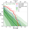 |
Fig. 3. Observed LF of M 83 (red line) compared to its Illustris-TNG50 analogs, with each analog corresponding to a gray line. The 1, 2, and 3σ confidence intervals are indicated with the green areas. The red numbers indicate the percentage of analogs that have more satellites than the observed one at a given step. Also shown is the Milky Way LF (blue), including (straight) and excluding (dashed) the rare Magellanic Clouds (MC). While the Milky Way LF without the MC is consistent with expectations from Illustris-TNG50, the M 83 LF deviates by more than 3σ. |
3.2. Subhalo mass function
We wanted to determined whether this finding is dependent on the cosmological simulation we used for our comparison. To check the robustness of our result, we followed a different approach. Instead of counting the number of simulated dwarf galaxies, we used the subhalo mass function (i.e., the mass distribution of dark halos that potentially host satellites around a host galaxy), providing the number of dark halos per mass unit for a given mass of the host galaxy (Schneider 2015). To estimate the satellite population around host galaxies, we attributed a stellar mass to each subhalo obtained (i.e., painting the dark matter subhalos with dwarf galaxies). Contrary to Milky Way-like galaxies, dwarf galaxies do not follow a well-defined stellar mass–halo mass relation (M⋆ − Msh). On the contrary, as seen in Fig. 2 of Sales et al. (2022), a large scatter exists for a given halo mass, showing a variation of up to three dex in luminosity for a given halo mass. This scatter reflects different build-up histories of dwarf galaxies and increases further when based on different models of galaxy formation that yield different results. To convert halo mass to stellar mass, we defined, based on Fig. 2 of Sales et al. (2022), a region in the M⋆ − Msh plot that encompasses all galaxies, either including only galaxies formed in the field or only satellite galaxies, that is, combining their Figs. 2a and 2b, which we depict in our Fig. 4. We chose the area such that it contains the largest number of luminous subhalos (i.e., potentially over-predicting the number of dwarf galaxies). For each subhalo, we randomly determined a luminosity from a uniform distribution spanning from the minimal to the maximal luminosity in this area for a given halo mass (corresponding to the shaded area in Fig. 4). As an example: a subhalo with a halo mass of 109 M⊙ can be assigned a stellar mass between ∼103 M⊙ and ∼5 × 10⁶ M⊙, which corresponds to the lower and upper value y values of the area at the x value of the halo mass in Fig. 4. We derived the LF of satellites as the cumulative number of satellites observed around a given galaxy. The scatter was estimated as 1, 2, and 3 standard deviations around the mean, which was obtained by averaging 300 realisations. For the halo mass of M 83, we used 0.8 × 10¹² solar masses (Karachentsev et al. 2007). These bounds are shown in Fig. 5, together with the observed LF of M 83.
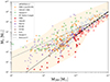 |
Fig. 4. Stellar to halo mass function adapted from Fig. 2 of Sales et al. (2022). The orange area was used in the sampling of the LF. Open symbols correspond to simulations of dwarf galaxies around a Milky Way-mass host halo from: APOSTLE-l1 (Sawala et al. 2016; Fattahi et al. 2016), FIRE:Latte/ELVIS (Wetzel et al. 2016; Garrison-Kimmel et al. 2019), NIHAO-UHD (Buck et al. 2019), Auriga-L3 (Grand et al. 2017), and DC Justice League (Munshi et al. 2021). Filled symbols correspond to zoom-in dwarf galaxies from: FIRE (Wheeler et al. 2015, 2019; Fitts et al. 2017), NIHAO (Wang et al. 2015), Marvel (Munshi et al. 2021), GEAR (Revaz & Jablonka 2018; Sanati et al. 2023), EDGE (Rey et al. 2019, 2020), and Jeon (Jeon et al. 2017). The dashed and dotted lines show abundance matching relations from Behroozi et al. (2013) and Moster et al. (2013), respectively. Note that their predictions are extrapolated below about 1010M200. |
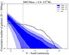 |
Fig. 5. Predicted cumulative number of satellites brighter than a given luminosity, within 300 kpc of M83, assuming a mass of 0.8 × 10¹² M⊙. The 1, 2, and 3σ confidence intervals are indicated with the blue areas. The black line corresponds to the LF of M 83. The vertical dashed line represents the survey limit of Müller et al. (2015). The M 83 LF deviates by more than 3σ from the subhalo mass function. |
At the bright end (i.e., > 5 × 10⁸ M⊙), the observed LF of M 83 is consistent with the predicted range of LFs at a 2σ level. However, this quickly starts to change at lower luminosities. At its maximum discrepancy – this is, between 107 and 108 M⊙ – the observed LF of M 83 differs by more than 5.5σ from the predictions given by this process of assigning dwarf galaxies to dark matter subhalos. This discrepancy is consistent with our previous finding from Illustris-TNG50 and puts the M 83 group at odds with ΛCDM. Increasing the halo mass to 1.0 × 10¹² (i.e., the Milky Way halo mass estimate) will still result in a 3σ discrepancy and does not alleviate the problem. Furthermore, this comparison again does not take into account that the observed LF may be underestimated by 20% due to incomplete observations. Including such a correction would only increase the tension.
4. Summary and conclusion
To study the LF of the M 83 group, we constructed a catalog of dwarf galaxies and employed distance measurements to confirm or reject eight dwarf galaxy candidate members from the literature. We were able to reject six of them, while two are too faint to get a good distance estimate. To be conservative, we assumed they were background objects. This left us with 13 confirmed dwarf galaxies in the M 83 group. We compared this dwarf galaxy sample to cosmological simulations, namely the Illustris-TNG50 project, as well as theoretical predictions from the subhalo mass function. By applying observational constraints to the simulated M 83 analogs in Illustris-TNG50, we derived the expected LFs. At the bright end, the LFs agree with the observed one. However, at the faint end, that is, in the luminosity range between 106 and 108 solar masses (i.e., −10 to −14 mag in the V band), all simulated M 83 analogs contained fewer satellites, and with 13 observed satellites within 330 kpc, the expectation was overshot by 3σ. The same is true when we used the subhalo mass function to predict the abundance of dwarf galaxies: we significantly underestimated the LF at the 5.5σ level for all galaxy formation models. Observational incompleteness may further increase this tension by ∼1σ because, even at the bright end, dwarf galaxies may not have been observationally detected due to the high density of foreground stars and contamination by galactic cirrus. The flattening of the observed LF at 106 solar masses indicates a further incompleteness, as we expect it would grow with a power law.
Modern cosmological simulations have been reported to more closely match the LF of the Milky Way, apparently resolving the classical missing-satellite problem. Yet, our results demonstrate that in the M 83 system, the number of satellites is underestimated at more than a 3σ level by such models, indicating that there is rather a too-many-satellites problem for the M 83 group. This implies that ΛCDM models do not seem to correctly predict the abundances (or physical properties) of dwarf galaxies for the full range of observed host galaxies in the nearby universe. In an extension of the work presented here, Kanehisa et al. (2023b) draw a similar conclusion at a higher significance level based on data from the MATLAS survey. These results should serve as a cautionary tale, highlighting the need to remain vigilant and to continue testing and improving models even when they can explain observations of our own Local Group.
Acknowledgments
We thank the referee for the constructive report, which helped to clarify and improve the manuscript. O. M. is grateful to the Swiss National Science Foundation for financial support under the grant numbers P400P2_191123 and PZ00P2_202104. M. S. P. acknowledges funding of a Leibniz-Junior Research Group (project number J94/2020). The authors thank Scott Carlsten for the help provided on the measurement of the surface brightness fluctuation. The authors further thank Azadeh Fattahi for providing us with the data points used in Fig. 4.
References
- Abazajian, K., Adelman-McCarthy, J. K., Agüeros, M. A., et al. 2003, AJ, 126, 2081 [Google Scholar]
- Abraham, R. G., & van Dokkum, P. G. 2014, PASP, 126, 55 [Google Scholar]
- Bacon, R., Accardo, M., Adjali, L., et al. 2010, SPIE Conf. Ser., 7735, 773508 [Google Scholar]
- Banks, G. D., Disney, M. J., Knezek, P. M., et al. 1999, ApJ, 524, 612 [NASA ADS] [CrossRef] [Google Scholar]
- Barnes, K. L., van Zee, L., Dale, D. A., et al. 2014, ApJ, 789, 126 [NASA ADS] [CrossRef] [Google Scholar]
- Beasley, M. A., Fahrion, K., & Gvozdenko, A. 2024, MNRAS, 527, 5767 [Google Scholar]
- Begum, A., Chengalur, J. N., Karachentsev, I. D., Sharina, M. E., & Kaisin, S. S. 2008, MNRAS, 386, 1667 [NASA ADS] [CrossRef] [Google Scholar]
- Behroozi, P. S., Wechsler, R. H., & Conroy, C. 2013, ApJ, 770, 57 [NASA ADS] [CrossRef] [Google Scholar]
- Bennet, P., Sand, D. J., Crnojević, D., et al. 2017, ApJ, 850, 109 [NASA ADS] [CrossRef] [Google Scholar]
- Bhardwaj, A. 2020, J. Astrophys. Astron., 41, 23 [NASA ADS] [CrossRef] [Google Scholar]
- Bird, S. A., Flynn, C., Harris, W. E., & Valtonen, M. 2015, A&A, 575, A72 [NASA ADS] [CrossRef] [EDP Sciences] [Google Scholar]
- Boylan-Kolchin, M., Bullock, J. S., & Kaplinghat, M. 2011, MNRAS, 415, L40 [NASA ADS] [CrossRef] [Google Scholar]
- Buck, T., Macciò, A. V., Dutton, A. A., Obreja, A., & Frings, J. 2019, MNRAS, 483, 1314 [NASA ADS] [CrossRef] [Google Scholar]
- Bull, P., Akrami, Y., Adamek, J., et al. 2016, Phys. Dark Universe, 12, 56 [NASA ADS] [CrossRef] [Google Scholar]
- Bullock, J. S., & Boylan-Kolchin, M. 2017, ARA&A, 55, 343 [Google Scholar]
- Carlsten, S. G., Beaton, R. L., Greco, J. P., & Greene, J. E. 2019a, ApJ, 879, 13 [NASA ADS] [CrossRef] [Google Scholar]
- Carlsten, S. G., Beaton, R. L., Greco, J. P., & Greene, J. E. 2019b, ApJS, 878, L16 [Google Scholar]
- Carlsten, S. G., Greene, J. E., Peter, A. H. G., Beaton, R. L., & Greco, J. P. 2021, ApJ, 908, 109 [NASA ADS] [CrossRef] [Google Scholar]
- Carlsten, S. G., Greene, J. E., Beaton, R. L., Danieli, S., & Greco, J. P. 2022, ApJ, 933, 47 [CrossRef] [Google Scholar]
- Carrillo, A., Bell, E. F., Bailin, J., et al. 2017, MNRAS, 465, 5026 [NASA ADS] [CrossRef] [Google Scholar]
- Cautun, M., Benítez-Llambay, A., Deason, A. J., et al. 2020, MNRAS, 494, 4291 [Google Scholar]
- Chiboucas, K., Karachentsev, I. D., & Tully, R. B. 2009, AJ, 137, 3009 [Google Scholar]
- Chiboucas, K., Jacobs, B. A., Tully, R. B., & Karachentsev, I. D. 2013, AJ, 146, 126 [Google Scholar]
- Crnojević, D., Grebel, E. K., & Cole, A. A. 2012, A&A, 541, A131 [NASA ADS] [CrossRef] [EDP Sciences] [Google Scholar]
- Crnojević, D., Sand, D. J., Caldwell, N., et al. 2014, ApJS, 795, L35 [Google Scholar]
- Crnojević, D., Sand, D. J., Spekkens, K., et al. 2016, ApJ, 823, 19 [Google Scholar]
- Crnojević, D., Sand, D. J., Bennet, P., et al. 2019, ApJ, 872, 80 [Google Scholar]
- Crosby, E., Jerjen, H., Müller, O., et al. 2023, MNRAS, 521, 4009 [Google Scholar]
- Da Costa, G. S., & Armandroff, T. E. 1990, AJ, 100, 162 [Google Scholar]
- Da Costa, G. S., Rejkuba, M., Jerjen, H., & Grebel, E. K. 2010, ApJ, 708, L121 [NASA ADS] [CrossRef] [Google Scholar]
- Dey, A., Schlegel, D. J., Lang, D., et al. 2019, AJ, 157, 168 [Google Scholar]
- Duc, P.-A., Cuillandre, J.-C., Karabal, E., et al. 2015, MNRAS, 446, 120 [Google Scholar]
- Dykes, T., Gheller, C., Koribalski, B. S., Dolag, K., & Krokos, M. 2021, Astron. Comput., 34, 100448 [NASA ADS] [CrossRef] [Google Scholar]
- Fattahi, A., Navarro, J. F., Sawala, T., et al. 2016, MNRAS, 457, 844 [NASA ADS] [CrossRef] [Google Scholar]
- Fitts, A., Boylan-Kolchin, M., Elbert, O. D., et al. 2017, MNRAS, 471, 3547 [NASA ADS] [CrossRef] [Google Scholar]
- For, B. Q., Staveley-Smith, L., Westmeier, T., et al. 2019, MNRAS, 489, 5723 [NASA ADS] [CrossRef] [Google Scholar]
- Garrison-Kimmel, S., Boylan-Kolchin, M., Bullock, J. S., & Kirby, E. N. 2014, MNRAS, 444, 222 [NASA ADS] [CrossRef] [Google Scholar]
- Garrison-Kimmel, S., Hopkins, P. F., Wetzel, A., et al. 2019, MNRAS, 487, 1380 [NASA ADS] [CrossRef] [Google Scholar]
- Grand, R. J. J., Gómez, F. A., Marinacci, F., et al. 2017, MNRAS, 467, 179 [NASA ADS] [Google Scholar]
- Grossi, M., Disney, M. J., Pritzl, B. J., et al. 2007, MNRAS, 374, 107 [NASA ADS] [CrossRef] [Google Scholar]
- Gwyn, S. D. J. 2008, PASP, 120, 212 [Google Scholar]
- Habas, R., Marleau, F. R., Duc, P.-A., et al. 2020, MNRAS, 491, 1901 [NASA ADS] [Google Scholar]
- Helmi, A., Babusiaux, C., Koppelman, H. H., et al. 2018, Nature, 563, 85 [Google Scholar]
- Herrmann, K. A., Ciardullo, R., Feldmeier, J. J., & Vinciguerra, M. 2008, ApJ, 683, 630 [Google Scholar]
- Huchtmeier, W. K., & Bohnenstengel, H. D. 1981, A&A, 100, 72 [NASA ADS] [Google Scholar]
- Ibata, R. A., Lewis, G. F., Conn, A. R., et al. 2013, Nature, 493, 62 [NASA ADS] [CrossRef] [Google Scholar]
- Javanmardi, B., Martinez-Delgado, D., Kroupa, P., et al. 2016, A&A, 588, A89 [NASA ADS] [CrossRef] [EDP Sciences] [Google Scholar]
- Javanmardi, B., Raouf, M., Khosroshahi, H. G., et al. 2019, ApJ, 870, 50 [NASA ADS] [CrossRef] [Google Scholar]
- Jeon, M., Besla, G., & Bromm, V. 2017, ApJ, 848, 85 [NASA ADS] [CrossRef] [Google Scholar]
- Jerjen, H., & Rejkuba, M. 2001, A&A, 371, 487 [NASA ADS] [CrossRef] [EDP Sciences] [Google Scholar]
- Kamphuis, P., Józsa, G. I. G., Oh, S. H., et al. 2015, MNRAS, 452, 3139 [NASA ADS] [CrossRef] [Google Scholar]
- Kanehisa, K. J., Pawlowski, M. S., & Müller, O. 2023a, MNRAS, 524, 952 [NASA ADS] [CrossRef] [Google Scholar]
- Kanehisa, K. J., Pawlowski, M. S., Heesters, N., & Müller, O. 2023b, A&A submitted [Google Scholar]
- Karachentsev, I. D., Sharina, M. E., Dolphin, A. E., et al. 2002, A&A, 385, 21 [CrossRef] [EDP Sciences] [Google Scholar]
- Karachentsev, I. D., Tully, R. B., Dolphin, A., et al. 2007, AJ, 133, 504 [NASA ADS] [CrossRef] [Google Scholar]
- Karachentsev, I. D., Makarov, D. I., Karachentseva, V. E., & Melnik, O. V. 2008, Astron. Lett., 34, 832 [NASA ADS] [CrossRef] [Google Scholar]
- Karachentsev, I. D., Makarov, D. I., & Kaisina, E. I. 2013, AJ, 145, 101 [Google Scholar]
- Koribalski, B. S., Staveley-Smith, L., Kilborn, V. A., et al. 2004, AJ, 128, 16 [Google Scholar]
- Kroupa, P., Famaey, B., de Boer, K. S., et al. 2010, A&A, 523, A32 [NASA ADS] [CrossRef] [EDP Sciences] [Google Scholar]
- Leavitt, H. S., & Pickering, E. C. 1912, Harvard College Obs. Circ., 173, 1 [NASA ADS] [Google Scholar]
- Lee, M. G., Freedman, W. L., & Madore, B. F. 1993, ApJ, 417, 553 [Google Scholar]
- Libeskind, N. I., Hoffman, Y., Tully, R. B., et al. 2015, MNRAS, 452, 1052 [NASA ADS] [CrossRef] [Google Scholar]
- McGaugh, S. S. 2005, ApJ, 632, 859 [Google Scholar]
- Meyer, M. J., Zwaan, M. A., Webster, R. L., et al. 2004, MNRAS, 350, 1195 [Google Scholar]
- Miyazaki, S., Komiyama, Y., Kawanomoto, S., et al. 2018, PASJ, 70, S1 [NASA ADS] [Google Scholar]
- Moore, B., Ghigna, S., Governato, F., et al. 1999, ApJS, 524, L19 [Google Scholar]
- Moster, B. P., Naab, T., & White, S. D. M. 2013, MNRAS, 428, 3121 [Google Scholar]
- Müller, O., & Jerjen, H. 2020, A&A, 644, A91 [NASA ADS] [CrossRef] [EDP Sciences] [Google Scholar]
- Müller, O., Jerjen, H., & Binggeli, B. 2015, A&A, 583, A79 [NASA ADS] [CrossRef] [EDP Sciences] [Google Scholar]
- Müller, O., Jerjen, H., & Binggeli, B. 2017a, A&A, 597, A7 [NASA ADS] [CrossRef] [EDP Sciences] [Google Scholar]
- Müller, O., Scalera, R., Binggeli, B., & Jerjen, H. 2017b, A&A, 602, A119 [NASA ADS] [CrossRef] [EDP Sciences] [Google Scholar]
- Müller, O., Jerjen, H., & Binggeli, B. 2018a, A&A, 615, A105 [Google Scholar]
- Müller, O., Rejkuba, M., & Jerjen, H. 2018b, A&A, 615, A96 [NASA ADS] [CrossRef] [EDP Sciences] [Google Scholar]
- Müller, O., Rejkuba, M., Pawlowski, M. S., et al. 2019, A&A, 629, A18 [Google Scholar]
- Müller, O., Fahrion, K., Rejkuba, M., et al. 2021, A&A, 645, A92 [NASA ADS] [CrossRef] [EDP Sciences] [Google Scholar]
- Müller, O., Heesters, N., Jerjen, H., Anand, G., & Revaz, Y. 2023, A&A, 673, A160 [NASA ADS] [CrossRef] [EDP Sciences] [Google Scholar]
- Munshi, F., Brooks, A. M., Applebaum, E., et al. 2021, ApJ, 923, 35 [NASA ADS] [CrossRef] [Google Scholar]
- Nelson, D., Springel, V., Pillepich, A., et al. 2019, Comput. Astrophys. Cosmol., 6, 2 [Google Scholar]
- Pawlowski, M. S. 2018, Mod. Phys. Lett. A, 33, 1830004a [CrossRef] [Google Scholar]
- Pawlowski, M. S. 2021, Nat. Astron., 5, 1185 [NASA ADS] [CrossRef] [Google Scholar]
- Pritzl, B. J., Knezek, P. M., Gallagher, J. S., III, et al. 2003, ApJS, 596, L47 [Google Scholar]
- Rejkuba, M. 2004, A&A, 413, 903 [NASA ADS] [CrossRef] [EDP Sciences] [Google Scholar]
- Revaz, Y., & Jablonka, P. 2018, A&A, 616, A96 [NASA ADS] [CrossRef] [EDP Sciences] [Google Scholar]
- Rey, M. P., Pontzen, A., Agertz, O., et al. 2019, ApJS, 886, L3 [Google Scholar]
- Rey, M. P., Pontzen, A., Agertz, O., et al. 2020, MNRAS, 497, 1508 [NASA ADS] [CrossRef] [Google Scholar]
- Roberts, D. M., Nierenberg, A. M., & Peter, A. H. G. 2021, MNRAS, 502, 1205 [NASA ADS] [CrossRef] [Google Scholar]
- Saifollahi, T., Trujillo, I., Beasley, M. A., Peletier, R. F., & Knapen, J. H. 2021, MNRAS, 502, 5921 [NASA ADS] [CrossRef] [Google Scholar]
- Sales, L. V., Wetzel, A., & Fattahi, A. 2022, Nat. Astron., 6, 897 [NASA ADS] [CrossRef] [Google Scholar]
- Sanati, M., Jeanquartier, F., Revaz, Y., & Jablonka, P. 2023, A&A, 669, A94 [NASA ADS] [CrossRef] [EDP Sciences] [Google Scholar]
- Sawala, T., Frenk, C. S., Fattahi, A., et al. 2016, MNRAS, 457, 1931 [Google Scholar]
- Sawala, T., Cautun, M., Frenk, C., et al. 2023, Nat. Astron., 7, 481 [Google Scholar]
- Schneider, A. 2015, MNRAS, 451, 3117 [NASA ADS] [CrossRef] [Google Scholar]
- Simon, J. D., & Geha, M. 2007, ApJ, 670, 313 [NASA ADS] [CrossRef] [Google Scholar]
- Simpson, C. M., Grand, R. J. J., Gómez, F. A., et al. 2018, MNRAS, 478, 548 [CrossRef] [Google Scholar]
- Smercina, A., Bell, E. F., Price, P. A., et al. 2018, ApJ, 863, 152 [NASA ADS] [CrossRef] [Google Scholar]
- Springel, V., Pakmor, R., Pillepich, A., et al. 2018, MNRAS, 475, 676 [Google Scholar]
- Taylor, M. A., Puzia, T. H., Muñoz, R. P., et al. 2017, MNRAS, 469, 3444 [NASA ADS] [CrossRef] [Google Scholar]
- Taylor, M. A., Eigenthaler, P., Puzia, T. H., et al. 2018, ApJS, 867, L15 [Google Scholar]
- Tollerud, E. J., Bullock, J. S., Strigari, L. E., & Willman, B. 2008, ApJ, 688, 277 [NASA ADS] [CrossRef] [Google Scholar]
- Tonry, J., & Schneider, D. P. 1988, AJ, 96, 807 [Google Scholar]
- van Dokkum, P., Danieli, S., Cohen, Y., et al. 2018, Nature, 555, 629 [Google Scholar]
- Wang, L., Dutton, A. A., Stinson, G. S., et al. 2015, MNRAS, 454, 83 [NASA ADS] [CrossRef] [Google Scholar]
- Weinberg, D. H., Bullock, J. S., Governato, F., Kuzio de Naray, R., & Peter, A. H. G. 2015, Proc. Nat. Acad. Sci., 112, 12249 [NASA ADS] [CrossRef] [Google Scholar]
- Wetzel, A. R., Hopkins, P. F., Kim, J.-H., et al. 2016, ApJS, 827, L23 [Google Scholar]
- Wheeler, C., Oñorbe, J., Bullock, J. S., et al. 2015, MNRAS, 453, 1305 [NASA ADS] [CrossRef] [Google Scholar]
- Wheeler, C., Hopkins, P. F., Pace, A. B., et al. 2019, MNRAS, 490, 4447 [CrossRef] [Google Scholar]
Appendix A: Dwarf galaxies around M 83
In Table A.1 we present the list of confirmed dwarf galaxies within 330 kpc of M 83.
Dwarf galaxies within a projected radius of 330 kpc around M 83.
Appendix B: Dwarf galaxy candidate dw1336-32
In Fig. B.1 we show a 6,000 s exposure in the g band with DECam (from program ID 2016A-0384) of the dwarf galaxy candidate dw1336-32 from Müller et al. (2015). It has a patchy morphology and is embedded in a cirrus-like structure, making it a likely false detection. No SBF is apparent. We reject it as a dwarf galaxy.
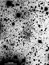 |
Fig. B.1. Deep single-band exposure of the dwarf galaxy candidate dw1336-32 in the g band, smoothed with a Gaussian kernel. |
All Tables
All Figures
|
Fig. 1. Color-composite images of previous dwarf galaxy candidates of M 83 that have an optical counterpart in deeper images. The galaxies that feature an SBF are labeled in green and objects without any SBF signal in red. |
| In the text | |
|
Fig. 2. Field around M 83. The large dot corresponds to M 83 and the small dots to confirmed dwarf galaxies. In color are dwarf galaxies with velocity measurements, in gray without. The thin circle corresponds to the virial radius of M 83 and the large circle to 330 kpc. |
| In the text | |
|
Fig. 3. Observed LF of M 83 (red line) compared to its Illustris-TNG50 analogs, with each analog corresponding to a gray line. The 1, 2, and 3σ confidence intervals are indicated with the green areas. The red numbers indicate the percentage of analogs that have more satellites than the observed one at a given step. Also shown is the Milky Way LF (blue), including (straight) and excluding (dashed) the rare Magellanic Clouds (MC). While the Milky Way LF without the MC is consistent with expectations from Illustris-TNG50, the M 83 LF deviates by more than 3σ. |
| In the text | |
|
Fig. 4. Stellar to halo mass function adapted from Fig. 2 of Sales et al. (2022). The orange area was used in the sampling of the LF. Open symbols correspond to simulations of dwarf galaxies around a Milky Way-mass host halo from: APOSTLE-l1 (Sawala et al. 2016; Fattahi et al. 2016), FIRE:Latte/ELVIS (Wetzel et al. 2016; Garrison-Kimmel et al. 2019), NIHAO-UHD (Buck et al. 2019), Auriga-L3 (Grand et al. 2017), and DC Justice League (Munshi et al. 2021). Filled symbols correspond to zoom-in dwarf galaxies from: FIRE (Wheeler et al. 2015, 2019; Fitts et al. 2017), NIHAO (Wang et al. 2015), Marvel (Munshi et al. 2021), GEAR (Revaz & Jablonka 2018; Sanati et al. 2023), EDGE (Rey et al. 2019, 2020), and Jeon (Jeon et al. 2017). The dashed and dotted lines show abundance matching relations from Behroozi et al. (2013) and Moster et al. (2013), respectively. Note that their predictions are extrapolated below about 1010M200. |
| In the text | |
|
Fig. 5. Predicted cumulative number of satellites brighter than a given luminosity, within 300 kpc of M83, assuming a mass of 0.8 × 10¹² M⊙. The 1, 2, and 3σ confidence intervals are indicated with the blue areas. The black line corresponds to the LF of M 83. The vertical dashed line represents the survey limit of Müller et al. (2015). The M 83 LF deviates by more than 3σ from the subhalo mass function. |
| In the text | |
|
Fig. B.1. Deep single-band exposure of the dwarf galaxy candidate dw1336-32 in the g band, smoothed with a Gaussian kernel. |
| In the text | |
Current usage metrics show cumulative count of Article Views (full-text article views including HTML views, PDF and ePub downloads, according to the available data) and Abstracts Views on Vision4Press platform.
Data correspond to usage on the plateform after 2015. The current usage metrics is available 48-96 hours after online publication and is updated daily on week days.
Initial download of the metrics may take a while.