| Issue |
A&A
Volume 691, November 2024
|
|
|---|---|---|
| Article Number | A71 | |
| Number of page(s) | 13 | |
| Section | Numerical methods and codes | |
| DOI | https://doi.org/10.1051/0004-6361/202348614 | |
| Published online | 30 October 2024 | |
VENICE: A multi-scale operator-splitting algorithm for multi-physics simulations
Leiden Observatory, University of Leiden,
Niels Bohrweg 2,
2333
CA
Leiden,
The Netherlands
e-mail: This email address is being protected from spambots. You need JavaScript enabled to view it.
★ Corresponding author; This email address is being protected from spambots. You need JavaScript enabled to view it.
Received:
15
November
2023
Accepted:
31
July
2024
Abstract
Context. We present VENICE, an operator-splitting algorithm to integrate a numerical model on a hierarchy of timescales.
Aims. VENICE allows a wide variety of different physical processes operating on different scales to be coupled on individual and adaptive time-steps. It therewith mediates the development of complex multi-scale and multi-physics simulation environments with a wide variety of independent components.
Methods. The coupling between various physical models and scales is dynamic, and realised through (Strang) operators splitting using adaptive time-steps.
Results. We demonstrate the functionality and performance of this algorithm using astrophysical models of a stellar cluster, first coupling gravitational dynamics and stellar evolution, then coupling internal gravitational dynamics with dynamics within a galactic background potential, and finally combining these models while also introducing dwarf galaxy-like perturbers. These tests show numerical convergence for decreasing coupling timescales, demonstrate how VENICE can improve the performance of a simulation by shortening coupling timescales when appropriate, and provide a case study of how VENICE can be used to gradually build up and tune a complex multi-physics model. Although the examples provided here couple dedicated numerical models, VENICE can also be used to efficiently solve systems of stiff differential equations.
Key words: methods: numerical
© The Authors 2024
 Open Access article, published by EDP Sciences, under the terms of the Creative Commons Attribution License (https://creativecommons.org/licenses/by/4.0), which permits unrestricted use, distribution, and reproduction in any medium, provided the original work is properly cited.
This article is published in open access under the Subscribe to Open model. This email address is being protected from spambots. You need JavaScript enabled to view it. to support open access publication.
1 Introduction
Improvements in computational capabilities over recent decades have allowed numerical models to increase in scale and complexity. This has mostly come in the form of models covering a range of physical processes (multi-physics models) and physical scales (multi-scale models).
Many multi-physics models use the concept of operatorsplitting. Instead of modelling all physical processes in concert, they are solved sequentially. Operator-splitting introduces a numerical error, but this error typically decreases as the timescale on which the operators are split decreases. If the operators are applied sequentially for the same time-steps, the error is linear in the time-steps. Applying the operators for fractional time-steps in interwoven patterns, much like a Verlet scheme Verlet (1967), results in quadratic errors in the time-step (e.g. Strang splitting, Strang 1968). Higher-order operator-splitting methods exist, but often in limited cases or non-trivial forms (Jia & Li 2011; Christlieb et al. 2015; Portegies Zwart et al. 2020a).
Even with traditional Strang splitting, all the operators are applied on roughly the same timescale, which necessarily must be the shortest common timescale of the system. In addition, the adopted time-step between two solvers is symmetric. As multi-physics models cover increasingly more physical processes, they tend to become increasingly more multi-scale as well. In addition, the range of scales in the problem may dramatically change with time. In that case, a time-step that dynamically varies with time and across coupling methods leads to considerable speed-up and smaller errors.
This issue of a large range of timescales has long been recognised in modelling systems with a large number of self-gravitating bodies (Aarseth 1985). In response, schemes were developed in which particles could be evolved on their individual, appropriate time-steps (Wielen 1967; McMillan 1986; Pelupessy et al. 2012). Additionally, the BRIDGE method (Fujii et al. 2007) has been developed to couple gravitationally interacting systems of different physical scales. It splits the combined (Hamiltonian) operator into two isolated, self-consistent systems and interaction terms. The two systems can be solved independently, using the preferred methods for each, but they interact on larger timescales. Although quite powerful, BRIDGE has several important shortcomings. These include its constant coupling timescale, the rigidity of coupled schemes used, and the fixation of the dataset on which each differential solver operates. As a consequence, the BRIDGE, once constructed, is rigid in the spatial and temporal domain, and in methodology. This rigidity limits its application in modern simulation endeavours.
With the gradual increase in the sophistication of domain-specific numerical solvers, it has become increasingly challenging to develop simulation models incorporating new physics and employing new algorithms. Expanding those models has also become more complex, because the higher sophistication renders the underlying numerical framework more fragile. Without thorough modularisation, we move in a direction in which simulation codes become unwieldingly complex.
In this paper, we introduce VENICE, an algorithm to split an arbitrary number of operators on a wide range of timescales. We explore the coupling of operators on dynamical, variable timescales, and discuss how BRIDGE is incorporated into the framework. We present a reference implementation in the AMUSE framework, using it to demonstrate the capabilities and measure the performance of the algorithm. VENICE improves performance in multi-physics simulations by allowing different components to couple at individually relevant timescales instead of the shortest common timescale. Possibly even more important than performance is the possibility of maintaining the framework, verifying its workings, and validating the results. An operational version including a research project using VENICE is presented in Huang et al. (2024), in which we develop a planet population synthesis analysis of planet formation in young stellar clusters. We start, however, with a brief overview of existing frameworks for addressing (astro)physical problems with their advantages and disadvantages.
2 A brief overview of multi-scale simulation frameworks
Portegies Zwart (2018) argues for a modular approach to multi-scale, multi-physics simulations. He envisions an environment in which highly optimised modules with a limited scope are combined, using a common interface, into a more complex framework that covers the full palette of physical processes at their appropriate scale, spatially and temporally. By incorporating at least two physically motivated solvers per domain, such a framework would subsequently comply with the “Noah’s Ark” philosophy for code-coupling paradigms (Portegies Zwart 2018). Having two or more solvers for addressing the same physical domain at the same spatial or temporal scale allows for independent verification and validation of the specific part of the simulation. While the whole purpose of performing numerical simulations is to go beyond what we can test from fundamental principles, a Noah’s Ark principle should be considered one of the fundamental aspects of a simulation framework environment.
We shall briefly discuss a number of such frameworks, which comply in part with the above criteria. A more extensive overview of such frameworks across disciplines is presented in Babur et al. (2015). Each of these frameworks has its advantages and focus area; for example, see Xianmeng et al. (2021) for simulating power plant reactors, DEM for computational fluid dynamics (Peters et al. 2018), aluminum electrolysis (Einarsrud et al. 2017), or artery dynamics in blood flow (Veen & Hoekstra 2020) (discussed below), and the general implicit coupling framework for multi-physics problems (Rin et al. 2017). The three frameworks that most closely comply with the listed requirements for a multi-purpose simulation environment include CACTUS, the multi-scale modelling framework, and AMUSE.
CACTUS (Goodale et al. 2003) is a general purpose problem-solving environment for the physical sciences (Allen et al. 2001). It is modular and supports parallel computing across the network with a variety of hardware. CACTUS was updated to version 4.12 in May 20221. CACTUS offers several advantages over other frameworks. It uses a component-based architecture, whereby the core functionality is provided by a central “flesh” and various “thorns” (modules) that can be independently developed, compiled, and loaded. The thorns can be parallelised for multi-core architectures and distributed computing environments. Its high level of abstraction and interoperability with other tools simplifies the development of complex simulations.
The closest philosophy to the AMUSE one is probably the Multiscale Modelling and Simulation Framework (MMSF, Borgdorff et al. 2013; Chopard et al. 2014), which has been applied in the MUSCLE3 environment (Veen & Hoekstra 2020). However, in contrast to AMUSE’s structure of a driver script instructing a set of models to run and exchange information, it instead manages a set of distributed, mostly independent models that exchange messages via externally configurable connections that block the messages if a result they need is not yet available.
The Astrophysics Multiphysics Simulation Environment (AMUSE for short, Portegies Zwart et al. 2009, 2013; Pelupessy et al. 2013) has similar advantages to CACTUS and the MMSF, and has the additional advantage of dynamic adaptation and a high-level programming interface. Although specifically designed for applications in astronomy, it branches out to oceanography and hydrology. While AMUSE provides the capability of coupling an arbitrary number of codes, it still relies on the coupling of an array of solvers with a second-order scheme with constant time-steps. The AMUSE framework provides a first implementation of Noah’s Ark, providing a pre-determined communication protocol with standardised rules and a common data model.
AMUSE adopts BRIDGE for its code-coupling to first, second, and even higher orders (Portegies Zwart et al. 2020a), but it fails when it comes to the time-dependent flexibility needed for modern multi-scale and multi-physics simulations. Part of this problem has been addressed in the NEMESIS module in AMUSE (van Elteren et al. 2019).
NEMESIS uses a global structure and sub-structures to couple the stars and planetary system dynamics through a cascade of BRIDGE patterns. The global structure contains stars and planets integrated by a direct N-body solver, while substructures are integrated using a symplectic N-body solver coupled to the global system via a symplectic BRIDGE Portegies Zwart et al. (2020b). Nemesis dynamically combines each planetary system’s direct, symplectic, and secular integrators at runtime. Escaping planets are removed from the local system and incorporated into the global N-body integrator, while the remaining planets continue with their native solver. This is a very dynamic environment in which codes are spawned and killed at runtime.
With VENICE, we go further into Noah’s Ark paradigm, by allowing an operator-based approach to code-coupling. By relaxing the coupling strategy and allowing for an arbitrary number of codes to be coupled with an arbitrary number of other codes with arbitrary coupling times makes VENICE more flexible, transparent, and modular than any of the above-mentioned endeavours.
3 Algorithm
We here discuss the generalised algorithm for a multi-scale operator approach.
3.1 Operator-splitting
The VENICE algorithm is based on the concept of operator-splitting. Consider a differential equation of the following form:
![Mathematical equation: $\[\frac{d y}{d t}=L_1(y)+L_2(y).\]$](/articles/aa/full_html/2024/11/aa48614-23/aa48614-23-eq1.png) (1)
(1)
The exact solution to this differential equation is
![Mathematical equation: $\[y(\Delta t)=e^{\left(\hat{L}_1+\hat{L}_2\right) \Delta t} y(0).\]$](/articles/aa/full_html/2024/11/aa48614-23/aa48614-23-eq2.png) (2)
(2)
An approximate solution would be
![Mathematical equation: $\[y(\Delta t)=e^{\hat{L}_1 \Delta t} e^{\hat{L}_2 \Delta t} y(0)+\mathcal{O}(\Delta t).\]$](/articles/aa/full_html/2024/11/aa48614-23/aa48614-23-eq3.png) (3)
(3)
This is equivalent to applying the separate operators in sequence. The error of this scheme is first order in the time-step. Strang (1968) developed a second-order scheme, of the following form:
![Mathematical equation: $\[y(\Delta t)=e^{\hat{L}_1 \Delta t / 2} e^{\hat{L}_2 \Delta t} e^{\hat{L}_1 \Delta t / 2} y(0)+\mathcal{O}\left(\Delta t^2\right).\]$](/articles/aa/full_html/2024/11/aa48614-23/aa48614-23-eq4.png) (4)
(4)
In this way, one can split two operators. In a multi-physics model, we often have more than two terms in an operator. Consider the following differential equation:
![Mathematical equation: $\[\frac{d y}{d t}=\sum_i l_i(y).\]$](/articles/aa/full_html/2024/11/aa48614-23/aa48614-23-eq5.png) (5)
(5)
We can split this operator by partitioning terms between suboperators ![Mathematical equation: $\[\hat{L}_1\]$](/articles/aa/full_html/2024/11/aa48614-23/aa48614-23-eq6.png) and
and ![Mathematical equation: $\[\hat{L}_2\]$](/articles/aa/full_html/2024/11/aa48614-23/aa48614-23-eq7.png) , and recursively splitting sub-operators consisting of more than one term. This retains the second-order scaling because no terms of 𝒪(Δt) are introduced.
, and recursively splitting sub-operators consisting of more than one term. This retains the second-order scaling because no terms of 𝒪(Δt) are introduced.
Partitioning between ![Mathematical equation: $\[\hat{L}_1\]$](/articles/aa/full_html/2024/11/aa48614-23/aa48614-23-eq8.png) and
and ![Mathematical equation: $\[\hat{L}_2\]$](/articles/aa/full_html/2024/11/aa48614-23/aa48614-23-eq9.png) can be done in a variety of ways, but the most practical one is to split off one term into
can be done in a variety of ways, but the most practical one is to split off one term into ![Mathematical equation: $\[\hat{L}_1\]$](/articles/aa/full_html/2024/11/aa48614-23/aa48614-23-eq10.png) and leave the rest in
and leave the rest in ![Mathematical equation: $\[\hat{L}_2\]$](/articles/aa/full_html/2024/11/aa48614-23/aa48614-23-eq11.png) . This minimises the number of operator applications; if L1 ever has to be split again, this has to be done twice, increasing the number of operators by four. If L2 has to be split, the number of operators only increases by two. For N operators, the split operator will then be of the following form:
. This minimises the number of operator applications; if L1 ever has to be split again, this has to be done twice, increasing the number of operators by four. If L2 has to be split, the number of operators only increases by two. For N operators, the split operator will then be of the following form:
![Mathematical equation: $\[\begin{aligned}y(\Delta t)= & e^{\hat{l}_1 \Delta t / 2} e^{\hat{l}_2 \Delta t / 2} \ldots e^{\hat{l}_{N-1} \Delta t / 2} e^{\hat{l}_N \Delta t} \times \\& e^{\hat{l}_{N-1} \Delta t / 2} \ldots e^{\hat{l}_2 \Delta t / 2} e^{\hat{l}_1 \Delta t / 2}.\end{aligned}\]$](/articles/aa/full_html/2024/11/aa48614-23/aa48614-23-eq12.png) (6)
(6)
3.2 Adaptive time operator-splitting
Strang splitting also naturally lends itself to adaptive time-stepping schemes. For this purpose, we separate operators into a slow set and a fast one with respect to a given time-step, Δt; a slow operator can be applied for Δt within some required tolerance, while a fast operator cannot. All slow operators can be partitioned into ![Mathematical equation: $\[\hat{L}_1\]$](/articles/aa/full_html/2024/11/aa48614-23/aa48614-23-eq13.png) and applied for Δt, and all fast operators can be partitioned into
and applied for Δt, and all fast operators can be partitioned into ![Mathematical equation: $\[\hat{L}_2\]$](/articles/aa/full_html/2024/11/aa48614-23/aa48614-23-eq14.png) . They might not be slow operators at Δt/2 either, but we can continue splitting the operators recursively until there are no more fast operators. Successively halving the time-step results in an exponential decrease, giving the algorithm a large dynamical range in timescales.
. They might not be slow operators at Δt/2 either, but we can continue splitting the operators recursively until there are no more fast operators. Successively halving the time-step results in an exponential decrease, giving the algorithm a large dynamical range in timescales.
Determining slow and fast operators is not trivial. It is not necessarily based only on how rapidly an operator works on its section of the data vector, but also on how other operators work on the same section of the data vector. A similar problem was considered by Jänes et al. (2014) for Newtonian gravity N-body models. They pointed out that even if all particles evolve rapidly (they gave the example of a cluster of hard stellar binaries that all evolve on the orbital timescale of the hard binaries), the interactions between stars in different binaries operate on timescales similar to those of single stars in the same cluster. They instead proposed an algorithm based on connected components and showed that it reduced the wall-clock run-time of a simulation of a cluster of hard binaries by up to two orders of magnitude, compared to older adaptive time-stepping schemes.
The algorithm would decompose the particles into subsystems given a set of particles, a definition of the interaction timescale, τG,ij, between two particles, i and j (e.g. the minimum of the flyby and free-fall times), and an evolution timescale, Δt. Within a subsystem, or connected component, each particle, i, would interact with at least one other particle, j, with τG,ij < Δt, while between two subsystems, there were no pairs, ij, with τG,ij < Δt. This does put particles with τG,ij > Δt in the same subsystem, but always because there is some path of particle pairs with timescales < Δt connecting the two.
In the Newtonian gravity N-body model, the flyby and freefall time were characteristic timescales that could be straightforwardly derived from the model. For other models, this may not be as simple. In VENICE, we leave this as a system parameter. Given N operators, this takes the form of a symmetric N × N matrix, τ, where τij = τji is the coupling timescale between operators ![Mathematical equation: $\[\hat{l}_i\]$](/articles/aa/full_html/2024/11/aa48614-23/aa48614-23-eq15.png) and
and ![Mathematical equation: $\[\hat{l}_j\]$](/articles/aa/full_html/2024/11/aa48614-23/aa48614-23-eq16.png) . Two uncoupled operators (for example, that describe system components that do not directly interact) have a coupling timescale of infinity; they can be applied for an arbitrarily large time-step, Δt, without having to be coupled2.
. Two uncoupled operators (for example, that describe system components that do not directly interact) have a coupling timescale of infinity; they can be applied for an arbitrarily large time-step, Δt, without having to be coupled2.
Decomposition into connected components results in a set, ![Mathematical equation: $\[\hat{C}_i\]$](/articles/aa/full_html/2024/11/aa48614-23/aa48614-23-eq17.png) , where each is a set consisting of > 1 operator (where operators within a
, where each is a set consisting of > 1 operator (where operators within a ![Mathematical equation: $\[\hat{C}_i\]$](/articles/aa/full_html/2024/11/aa48614-23/aa48614-23-eq18.png) interact on timescales < Δt, but operators in different
interact on timescales < Δt, but operators in different ![Mathematical equation: $\[\hat{C}_i\]$](/articles/aa/full_html/2024/11/aa48614-23/aa48614-23-eq19.png) s do not), and a rest set,
s do not), and a rest set, ![Mathematical equation: $\[\hat{R}\]$](/articles/aa/full_html/2024/11/aa48614-23/aa48614-23-eq20.png) , of operators that are not connected to any other (and that do not interact with operators on timescales < Δt). Each connected component,
, of operators that are not connected to any other (and that do not interact with operators on timescales < Δt). Each connected component, ![Mathematical equation: $\[\hat{C}_i\]$](/articles/aa/full_html/2024/11/aa48614-23/aa48614-23-eq21.png) , is fast compared to Δt, and has to be partitioned in
, is fast compared to Δt, and has to be partitioned in ![Mathematical equation: $\[\hat{L}_1\]$](/articles/aa/full_html/2024/11/aa48614-23/aa48614-23-eq22.png) . The operators in the rest set,
. The operators in the rest set, ![Mathematical equation: $\[\hat{R}\]$](/articles/aa/full_html/2024/11/aa48614-23/aa48614-23-eq23.png) , are all slow compared to Δt, and can be partitioned into
, are all slow compared to Δt, and can be partitioned into ![Mathematical equation: $\[\hat{L}_2\]$](/articles/aa/full_html/2024/11/aa48614-23/aa48614-23-eq24.png) . This results in the following partitioning:
. This results in the following partitioning:
![Mathematical equation: $\[\frac{d y}{d t}=e^{\left(\Sigma_i \hat{C}_i \Delta t / 2\right)} e^{(\hat{R} \Delta t)} e^{\left(\sum_i \hat{C}_i \Delta t / 2\right)}.\]$](/articles/aa/full_html/2024/11/aa48614-23/aa48614-23-eq25.png) (7)
(7)
The operators in the rest set, R, and the connected sets of operators, C1 ..CK, must again be split, which can be done by linear splitting (Eq. (3)) or Strang splitting (Eq. (4)). Then, each individual Ci can again be split into connected components. It should be noted that if the connected components, Ci, are split by Strang splitting, one is split at Δt/2, while the others are split at Δt/4.
In Algorithm 1, we show the basic VENICE algorithm. For simplicity, we first use order splitting of the set C1 ...CK and of R.
1: procedure EVOLVE_CC(L, Δt, τ)
2: ⊳ Split codes into connected components
3: C1 ..CK, R = SPLIT_CC(L, Δt, τ)
4: ⊳ Evolve connected components for half time
5: for Ci in C1..Ck do
6: EVOLVE_CC(Ci, Δt/2, τ)
7: end for
8: ⊳ Evolve rest codes for full time
9: for li in R do
10: EVOLVE(li, Δt)
11: end for
12: ⊳ Evolve connected components
13: ⊳ for another half time
14: for Ci in C1..Ck do
15: EVOLVE_CC(Ci, Δt/2, τ)
16: end for
17: end procedure
In Fig. 1, we show an illustration of a system of 11 operators, coupled on different (unit-less for clarity) timescales. This system decomposes into two subsystems at Δt = 2−2 ≡ 0.25, meaning that the two subsystems exchange information with an interval of 0.25. Most of the operators in these subsystems are then split at a time-step of Δt = 2−5 ≈ 0.03, except for operators 6 and 7, which are more tightly coupled and only split at a time-step of Δt = 2−8 ≈ 0.004.
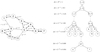 |
Fig. 1 Timescale matrix for a VENICE implementation. Left: representation of the coupling timescale matrix, τ, of an operator set as an undirected, weighted graph. Edges are labelled with the coupling timescale; some edges between triangulated nodes share labels for clarity. The coupling timescale between unconnected nodes is ∞. Right: tree representation of the recursive splitting of connected components, for the system on the left. Dotted lines denote skipped layers of nodes with a single parent and child node. |
3.3 Kick interactions
The BRIDGE scheme was introduced by Fujii et al. (2007) in order to couple different gravitational systems, such as stellar clusters within a galaxy. It uses operator-splitting to split the system into individual subsystems and interaction terms, each with their own time-steps. In this way, a stellar cluster’s internal dynamics can be solved on a shorter timescale than the cluster’s orbit in the galaxy, or the dynamics of the galaxy. This method was expanded by Pelupessy & Portegies Zwart (2012) to also allow gravitational coupling with smoothed-particle hydrodynamical models. Portegies Zwart et al. (2020a) have expanded the method to higher-order coupling and introduced augmented coupling patterns that allow for external forces (e.g. the YORP effect and general relativity into an otherwise Newtonian solver). We discuss how such a splitting can be incorporated into VENICE.
A bridged system can be seen as the following operator:
![Mathematical equation: $\[l_i=\sum_j\left(l_i^{(j)}+\sum_k \tilde{l}_i^{(j k)}\right),\]$](/articles/aa/full_html/2024/11/aa48614-23/aa48614-23-eq26.png) (8)
(8)
where ![Mathematical equation: $\[y_i^{(j)} \cap y_i^{(k)}=0 \quad \boldsymbol{\forall} \quad j \neq k\]$](/articles/aa/full_html/2024/11/aa48614-23/aa48614-23-eq27.png) ; in other words, all
; in other words, all ![Mathematical equation: $\[l_i^{(j)}\]$](/articles/aa/full_html/2024/11/aa48614-23/aa48614-23-eq28.png) use and change a different subvector of yi. These are the individual N-body systems. The operators,
use and change a different subvector of yi. These are the individual N-body systems. The operators, ![Mathematical equation: $\[\tilde{l}_i^{(j k)}\]$](/articles/aa/full_html/2024/11/aa48614-23/aa48614-23-eq29.png) , however, use both
, however, use both ![Mathematical equation: $\[y_i^{(j)}\]$](/articles/aa/full_html/2024/11/aa48614-23/aa48614-23-eq30.png) and
and ![Mathematical equation: $\[y_i^{(k)}\]$](/articles/aa/full_html/2024/11/aa48614-23/aa48614-23-eq31.png) , but affect only
, but affect only ![Mathematical equation: $\[y_i^{(j)}\]$](/articles/aa/full_html/2024/11/aa48614-23/aa48614-23-eq32.png) . These are the kick interactions that work on N-body system j.
. These are the kick interactions that work on N-body system j.
If we split the kick interactions, ![Mathematical equation: $\[\hat{\tilde{l}}_i^{(j k)}\]$](/articles/aa/full_html/2024/11/aa48614-23/aa48614-23-eq33.png) , into L1 and the evolutions,
, into L1 and the evolutions, ![Mathematical equation: $\[\hat{l}_i^{(j)}\]$](/articles/aa/full_html/2024/11/aa48614-23/aa48614-23-eq34.png) , into L2, we obtain the following second-order operatorsplitting (also see Portegies Zwart et al. 2020a, for higher-order couplings):
, into L2, we obtain the following second-order operatorsplitting (also see Portegies Zwart et al. 2020a, for higher-order couplings):
![Mathematical equation: $\[\begin{aligned}e^{l_i \Delta t}= & \left(\prod_j \prod_k e^{\hat{\tilde{l}}_i^{(jk)} \Delta t / 2}\right)\left(\prod_j e^{\hat{l}_i^{(j)} \Delta t}\right) \\& \times\left(\prod_j \prod_k e^{\hat{\tilde{l}}_i^{(j k)} \Delta t / 2}\right).\end{aligned}\]$](/articles/aa/full_html/2024/11/aa48614-23/aa48614-23-eq35.png) (9)
(9)
If an operator equivalent to a bridged system is present, it can be desirable to split it explicitly for flexibility and transparency. The individual operators, ![Mathematical equation: $\[l_i^{(j)}\]$](/articles/aa/full_html/2024/11/aa48614-23/aa48614-23-eq36.png) , can be treated much in the same way as other operators, li, but the kick operators,
, can be treated much in the same way as other operators, li, but the kick operators, ![Mathematical equation: $\[\tilde{l}_i^{(j k)}\]$](/articles/aa/full_html/2024/11/aa48614-23/aa48614-23-eq37.png) , require special treatment. Formally, they must be applied directly before and after the bridged operators, without any other, non-bridged operator in between. However, this becomes impossible when a bridged subsystem is also coupled to another operator on a shorter timescale3. In that case, the other operator must be included in the second factor of Eq. (9), and that factor must be decomposed into connected components following Eq. (7).
, require special treatment. Formally, they must be applied directly before and after the bridged operators, without any other, non-bridged operator in between. However, this becomes impossible when a bridged subsystem is also coupled to another operator on a shorter timescale3. In that case, the other operator must be included in the second factor of Eq. (9), and that factor must be decomposed into connected components following Eq. (7).
The question now is where to apply kick operators. We propose to place them between the evolution of the connected components and the rest set. This preserves Strang splitting if two operators are in different connected components. This is most obvious if both are in the rest set, where two kick operators flank the evolution operators. If both are in different Cis, the kick operators are applied without evolution operators in between, which instead are applied for half a time-step before and after the kick operators. This preserves the second-order BRIDGE scheme.
3.4 Dynamic coupling timescales
The decomposition of operators into connected components happens in every recursive evaluation, including those that happen after some operators have been (partly) applied. This means that if the timescale matrix, τij, were to change as the system evolves, the structure of the connected components could also change. In this way, VENICE can create a time-stepping scheme that adapts to the behaviour of the system. For example, if one operator represents stellar evolution, this operator can be coupled on long timescales so long as all stars remain on the main sequence, on shorter timescales when one or more stars move to more rapidly evolving stages of evolution, and then again on longer timescales when those stars become inert stellar remnants.
The coupled system remains consistent (with all operators applied for the same total time) so long as the connected components within one recursive function call of EVOLVE_CC (see Algorithm 1) are not changed (i.e. operators, li, do not move between different connected components, Ci, and/or the rest set, R). However, between two subsequent recursive function calls of EVOLVE_CC of a connected component, Ci, the decomposition into further connected components may be different.
In Algorithm 2, we show the VENICE algorithm extended with kick interactions and dynamic coupling timescales. For clarity, we present the algorithm with first-order splitting of R and the set C1 ..CK.
3.5 AMUSE implementation
Thus far, we have discussed VENICE as an operator-splitting algorithm. However, it can also be used as a coupling scheme for physical models that may not strictly solve a proper partial differential equation. The AMUSE platform provides a standardised structure for (interfaces to) physical models, making it an excellent environment to develop a reference implementation of the algorithm.
In the previous sections, we tacitly assumed that all operators affect the same data vector. However, in AMUSE every code has its own data vector (typically in the form of particle or grid data). Coupling must be done explicitly, by copying data from one code to another. In this implementation, we use the channels in AMUSE. These are defined from one data structure to another, and can copy any subset of data from one structure to the other. They must be explicitly called, which we do between operations. We could have chosen a lazy approach, whereby before the evolution of a code we copy all channels to that code. However, this results in an end state in which the data of different codes is different, and it is non-trivial to reconstruct which code contains the most recent state. Instead, we take an active approach, whereby we copy all channels from a code after its evolution step. This can introduce unnecessary copy operations, but is less prone to mistakes.
In many situations, the structure of a code’s dataset will be updated throughout the simulation (e.g. adaptive mesh refinement codes, particle-based stellar winds, and sink particles). To resolve this, every pair of codes can have a function that synchronises the datasets, defined by the user. This is done before channels are copied to ensure the data structures are compatible.
We also implemented a data output framework. This allows for analysis of fast subsystems without needing the same short time-step for the entire system (or the construction of a wrapper class whose only purpose besides evolving is writing data). We write three types of output: checkpoint files, plot files, and debug files. Checkpoint files are saved after the evolution of all codes, and contain the state of the entire system at a synchronised time. Plot files are saved after the evolution of an entire connected component. To prevent redundant files, saving checkpoint and plot files is skipped if there is only a single connected component, consisting of more than one code; in that case, the state at the end of the function is the same as at the end of the second recursive call. Debug files are saved after the evolution of individual codes.
The AMUSE implementation is available on Github4.
4 Testing VENICE
In this section, we present a number of tests of VENICE using the AMUSE implementation. The scripts to run these tests and produce the figures are also available on the VENICE Github page.
4.1 Gravity and stellar evolution
Coupled gravity-stellar evolution simulations are one of the oldest types of astrophysical multi-physics simulations, going back to Terlevich (1987). The coupling of these systems is relatively straightforward. Assuming a collisionless system and no changes in momentum during stellar evolution (e.g. supernova kicks), the only coupling is through the mass. Stars lose mass in stellar winds and at the end of their lifetime, and this changes the gravitational acceleration that they induce in other stars. Newton’s equations of motion can account for changing mass in differential form, but most astrophysical gravitational dynamics models do not include this. Coupling is typically done through operator-splitting.
We used the PH4 (McMillan et al. 2012) gravitational dynamics code and the SEBA parameterised stellar evolution code (Portegies Zwart & Verbunt 1996; Toonen et al. 2012). Coupling was done through a channel copying mass from the stellar evolution code to the gravitational dynamics code.
In Sect. 4.1.1, we use a constant coupling timescale. This becomes problematic if the stellar evolution timescale changes. This happens, for example, when a star leaves the main sequence. In Sect. 4.1.2, we expand the model with a dynamic coupling timescale.
For the initial conditions, we adopted a 100-star Plummer sphere in virial equilibrium. Stellar masses are distributed following a Kroupa initial mass function (IMF) (Kroupa 2001) between 0.08 and 8 M⊙. We manually set a randomly selected star to a higher mass, 16 M⊙ in Sect. 4.1.1 and 50 M⊙ in Sect. 4.1.2. The Plummer radius was set such that the free-fall time is 6 Myr (resulting in a Plummer radius of ~1.25 pc with the 16 M⊙ star, and ~1.47 pc with the 50 M⊙ star). This is also the total run-time of the tests. During this time, the 16 M⊙ star remains on the main sequence, and loses relatively little mass, allowing us to use relatively long coupling timescales compared to the total simulation time. The 50 M⊙ star leaves the main sequence and undergoes a supernova explosion during this time frame. This results in more rapid changes in mass, requiring very short coupling timescales at certain epochs. In Sect. 4.1.2, we demonstrate a timescale update function that can shorten the coupling timescale appropriately.
1: procedure EVOLVE_CC(L, Δt, τ)
2: ⊳ Update coupling timescales
3: UPDATE_TIMESCALES(L, Δt, τ)
4: ⊳ Split codes into connected components
5: C1 ..CK, R = SPLIT_CC(L, Δt, τ)
6: ⊳ Evolve connected components for half time
7: for Ci in C1 ..Ck do
8: EVOLVE_CC(Ci, Δt/2, τ)
9: end for
10: ⊳ Kick between connected components for half time
11: for li in l do
12: for lj in l do
13: if li and lj not in same Ck then
14: KICK(li, lj, Δt/2)
15: end if
16: end for
17: end for
18: ⊳ Evolve rest codes for full time
19: for li in R do
20: EVOLVE(li, Δt)
21: end for
22: ⊳ Kick between connected components for another half time
23: for li in l do
24: for lj in l do
25: if li and lj not in same Ck then
26: KICK(li, lj, Δt/2)
27: end if
28: end for
29: end for
30: ⊳ Evolve connected components for another half time
31: for Ci in C1..Ck do
32: EVOLVE_CC(Ci, Δt/2, τ)
33: end for
34: end procedure
4.1.1 Constant coupling timescale
In Pseudocode 1, we show how a VENICE system of gravitational dynamics and stellar evolution coupled at a constant timescale is set up.
1: procedure SETUP_GRAVITY_STELLAR_CONSTANT(gravity, stellar, dt)
2: system = VENICE()
3: system.ADD_CODE(gravity)
4: system.ADD_CODE(stellar)
5: system.timescale_matrix[0][1] = dt
6: ⊳ Copy mass from code 1 (stellar)
7: ⊳ to 0 (gravity)
8: system.ADD_CHANNEL(1, 0, [“mass”])
9: return system
10: end procedure
In Fig. 2, we show three views of the median position error, coupling timescale, and wall-clock run-time as functions of each other, for both first- and second-order splitting of the operator rest set, R (the splitting order of the connected components, C1 ...CK, does not affect the splitting procedure for <4 operators). We also show the time evolution of the median position error. The position error was defined as the distance between initially identical particles in runs with different timescales. We computed position errors between subsequent values of the coupling timescale, indicated by the end points of error bars.
Most gravitational systems of more than two bodies are chaotic (Miller 1964). As a result, any perturbation we introduce in the system triggers an exponential growth of that perturbation. Changing the timescale from one run to another is such a perturbation, and therefore triggers exponential growth. We observe that the median position error grows roughly linearly with time (although this may be the first-order behaviour of exponential growth at times much smaller than the Lyapunov time), and that there is a systematic offset between curves associated with subsequent coupling timescales. Therefore, we argue that the systematic change is caused by the coupling timescale, and not by the chaotic behaviour of the system.
The median position error scales approximately linearly with the coupling timescale, for both first- and second-order coupling. However, at the same time-step the error of the second-order method is an order of magnitude smaller. This comes at the cost of slightly longer wall-clock run-time5 but the median position error at a given run-time is typically lower for the second order than for the first order. In this model configuration (where the gravity model is the first element of the operator list, L), it is the gravity model that is evolved in two steps due to Strang splitting. This can be explained by the gravity model’s preferred internal time-step being larger than the largest coupling timescale, so that it performs a single numerical step every time VENICE evolves the model. In this case, the gravity model does not dominate the computation time, so the increase in run-time is small. This implies that second-order coupling results in the best trade-off between run-time and performance unless both models have a comparable run-time and have to shorten their internal time-step.
The order in which operators are split affects the outcome of numerical integration. To quantify this effect, we compare the model above with a model that is identical, except that the stellar evolution model is the first operator in L. This is done by reversing the order of ADD_CODE calls in Pseudocode 1, and results in the stellar evolution model being evolved twice per Strang splitting, instead of the gravity model. In Fig. 3, we show how the median position error and the wall-clock run-time depend on the coupling timescale, for the two reversed models, at the same coupling timescale, for both first- and second-order coupling.
We observe globally the same behaviour as for the convergence with timescale; the median position errors converges linearly with the timescale, for both first- and second-order coupling, although second-order coupling results in smaller errors. The magnitude of the errors are also roughly the same at a given coupling timescale. Finally, we again see that the code being evolved twice has a longer run-time6. This shows that the order of operators impacts the efficiency of the model, and while it also impacts the results, this error converges with shorter coupling timescales.
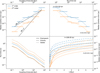 |
Fig. 2 Convergence and performance of a gravitational dynamics model and a stellar evolution one, coupled at a constant timescale. The top panels and the bottom left panel show three views of the median position error, coupling timescale, and wall-clock run-time as functions of each other. The bottom right panel shows the time evolution of the median position error in all runs. The dashed black lines in the top left plot show linear and quadratic scalings of the error with the timescale. |
4.1.2 Adaptive coupling timescale
In the test above, we were able to achieve a numerically converging solution at relatively long coupling timescales because no star evolved off the main sequence during the integration time. Off the main sequence, stars evolve rapidly, ultimately going supernova on a stellar free-fall time, or shedding their envelopes as planetary nebulae. Evolving the entire system at the shortest possible timescale at which the stellar population can evolve would result in a large overhead, leading to many unnecessary couplings. VENICE can easily resolve this using an UPDATE_TIMESCALE function. Setting this to some fraction, η, of the evolution timescale of the fastest-evolving star allows the system to couple more frequently when needed.
In principle, the most efficient integration would be achieved by coupling every star on its own timescale; the scheme we described evolves all stars, including those on the main sequence, on the timescale of the star with the shortest time-step. However, this increases the overhead of VENICE (note that the connected component algorithm scales quadratically with the number of operators). The optimal solution is to separate stars into a number of mass bins, but calibrating the optimal method of distribution is beyond the scope of this work.
In Pseudocode 2, we show how a VENICE system of gravitational dynamics and stellar evolution coupled at a dynamic timescale is set up.
We used the same initial conditions as in the previous section, except with a 50 M⊙ star instead of a 16 M⊙ one, and re-scaling the cluster radius and stellar velocities such that the dynamical time is still 6 Myr.
In Fig. 4, we show the median position error (top) and the wall-clock run-time (bottom) as a function of the coupling timescale parameter, η, for both first- and second-order coupling. The median position error scales roughly linearly for both first- and second-order coupling, but the error does not monotonically scale with the timescale parameter. The increase in run-time in second-order coupling is again due to gravity being split into two evolution steps.
1: procedure SETUP_GRAVITY_STELLAR_ADAPTIVE(gravity, stellar, η)
2: system = VENICE()
3: system.ADD_CODE(gravity)
4: system.ADD_CODE(stellar)
5: ⊳ lambda defines a function, as in Python
6: system.update_timescale[0][1] =
7: lambda code1, code2, dt:
8: η * code2.stellar_timesteps.MIN()
9: ⊳ Copy mass from code 1 (stellar)
10: ⊳ to 0 (gravity)
11: system.ADD_CHANNEL(l, 0, [“mass”])
12: return system
13: end procedure
In Fig. 5, we show how the coupling timescale evolves as a function of time for a number of values of η (top), and the stellar type of the 50 M⊙ star (bottom) over the same time interval. Over the first 4 Myr, the star is on the main sequence and the coupling timescale is mostly constant. At a number of transitions between phases (before and after the Hertzsprung gap and giant branch naked helium star phases, sometimes called “stripped stars”, these days), the coupling timescale drops by up to seven orders of magnitude, but also quickly increase by orders of magnitude afterwards. Then, when the star is a black hole, the coupling timescale becomes the same for values of η ≥ 0.1. This indicates that the coupling timescale dictated by the stellar evolution model is large compared to the remaining integration time.
We note that for η > 1, the model has a tendency to “overshoot” phases of stellar evolution. Ideally, the ratio of coupling timescales for two values of η should always be about η itself, but during, for example, the transition from the Hertzsprung gap to core helium-burning for η = 10, and the transition from giant branch naked helium star to black hole for η = 3, 10, the sharp drop to coupling timescales ≪1 kyr does not occur, while for higher values of η it does. In these cases, the stellar evolution model evolves through the rapid evolution phase without recomputing the coupling timescale. This implies that values of η ≲ 1 should be used.
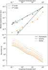 |
Fig. 3 Convergence and performance of a gravitational dynamics and stellar evolution model coupled at a constant timescale, with reversed operators. We show, as a function of the coupling timescale, the median position error (top) and wall-clock run-time (bottom). The dashed black lines in the top plot show linear and quadratic scalings of the error with the timescale. |
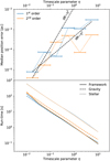 |
Fig. 4 Convergence and performance of a gravitational dynamics and a stellar evolution model coupled at an adaptive timescale. We show, as a function of the timescale parameter, η, the median position error (top) and wall-clock run-time (bottom). The median position error was computed for two subsequent values of the coupling timescale, indicated by the endpoints of the error bars. The dashed black lines in the top plot show linear and quadratic scalings of the error with the timescale. |
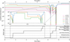 |
Fig. 5 Evolution of the dynamic coupling time-scales. Top: dynamic coupling timescale between the gravitational dynamics and stellar evolution models as a function of time, for a number of timescale parameters, η. Bottom: the stellar type through time of a 50 M⊙ star, which is the most massive one in the system of the top panel. |
4.2 BRIDGE d gravity
We demonstrate the BRIDGE algorithm in VENICE by simulating the dynamics of a star cluster in a galaxy.
The cluster consists of 100 stars, with masses drawn from a Kroupa IMF between 0.08 and 8 M⊙, distributed following a Plummer distribution with a radius of 10 pc. We again used PH4 to model the cluster’s gravitational dynamics.
We coupled this cluster to the analytic Bovy (2015) Milky-Way-like galaxy potential, which consists of a bulge (power law, exponentially cut-off density profile), disc (Miyamoto-Nagai density profile, Miyamoto & Nagai 1975), and halo (NFW density profile, Navarro et al. 1996).
We initialised the cluster at 8 kpc from the centre of the galaxy, with a velocity perpendicular to the direction to the centre. We parameterised this velocity in terms of an effective eccentricity: the velocity is that of a Keplerian orbit, at apocenter, for a central mass equal to the total mass within a circular orbit, given the effective eccentricity. If this eccentricity is 0, the orbit will be circular, but larger effective eccentricities do not result in elliptic orbits (because the mass enclosed in the orbit is not constant). We evolved the system for 223 Myr, one period of the adopted orbit.
4.2.1 Classical BRIDGE
In Pseudocode 3, we show how a VENICE system of two bridged gravitational dynamics models, coupled at a constant timescale, is set up. In this case, code 0 is the galaxy potential and code 1 is the cluster gravity.
We set the cluster’s orbital velocity such that the effective eccentricity is 0. In these tests, we used the cluster’s centre of mass to investigate the system’s convergence.
In Fig. 6, we show how the centre of mass error (top) and wall-clock run-time (bottom) depend on the coupling timescale. Because the only coupling is done through kick interactions (and there is no shared data between the gravity codes), the splitting order of the operator rest set, R, should not affect the result. For this reason, we only show the result of first-order splitting. However, we note that by construction the BRIDGE scheme has second-order error behaviour.
1: procedure SETUP_BRIDGED_GRAVITY_CONSTANT(grav-ity1, gravity2, dt)
2: system = VENICE()
3: system.ADD_CODE(gravity1)
4: system.ADD_CODE(gravity2)
5: system.timescale_matrix[0][1] = dt
6: ⊳ Kick interactions from code 0 to code 1
7: system.kick[0][1] = dynamic_kick
8: return system
9: end procedure
The position error indeed scales quadratically with the coupling timescale. Towards long coupling timescales, the run-time of the cluster gravity model appears to move towards an asymptote. This is the point at which the code no longer requires shortened time-steps to fit within the coupling timescale, but can take large internal time-steps.
4.2.2 Adaptive BRIDGE
Analogous to the time-step in the general N-body problem, the bridge time-step can potentially cover a large range. If a star cluster’s orbit within a galaxy is not circular, the appropriate bridge time-step can be smaller close to the galactic centre than farther away.
We based the adaptive coupling timescale on the freefall times of the particles in one model in the potential of the other model. The freefall time between two particles, i and j, is ![Mathematical equation: $\[\sqrt{r_{i j} / a_{i j}}\]$](/articles/aa/full_html/2024/11/aa48614-23/aa48614-23-eq38.png) , where rij is the distance between the particles and aij is the gravitational acceleration. The acceleration was computed for the BRIDGE interaction, and the distance is that to the centre of the central potential. Similar to the dynamic stellar coupling timescale, we next took the minimum among all particles and applied a scaling factor, η. We used the initial conditions described above, and set the cluster’s velocity such that the effective eccentricity is 0.5.
, where rij is the distance between the particles and aij is the gravitational acceleration. The acceleration was computed for the BRIDGE interaction, and the distance is that to the centre of the central potential. Similar to the dynamic stellar coupling timescale, we next took the minimum among all particles and applied a scaling factor, η. We used the initial conditions described above, and set the cluster’s velocity such that the effective eccentricity is 0.5.
1: procedure SETUP_BRIDGED_GRAVITY_ADAPTIVE(gravity 1, gravity2, η)
2: system = VENICE()
3: system.ADD_CODE(gravity1)
4: system.ADD_CODE(gravity2)
5: system.update_timescale[0][1] =
6: lambda code1, code2, dt:
7: η * MIN_FREEFALL_TIME(code1, code2)
8: ⊳ Kick interactions from code 0 to code 1
9: system.kick[0][1] = dynamic_kick
10: return system
11: end procedure
In Fig. 7, we show how the centre of mass error (top) and wall-clock run-time (bottom) depend on the coupling timescale parameter, η. Similarly to the case of the constant coupling timescale, the centre of mass error converges quadratically with the coupling timescale parameter, and the cluster gravity runtime no longer decreases at large coupling timescales. We note that the centre of mass error between η = 0.3 and η = 1 is larger than the initial distance from the galactic centre, while between η = 0.1 and η = 0.3 it is almost two orders of magnitude smaller than the initial distance. This implies that a value of η < 1 should be used.
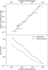 |
Fig. 6 Centre of mass error (top) and wall-clock run-time (bottom) as a function of constant coupling timescale, for a star cluster in a background galaxy potential. Centre of mass errors were computed between subsequent values of the coupling timescale, indicated by the ends of the error bars. The dashed black line indicates quadratic scaling of the centre of mass error with the coupling timescale. |
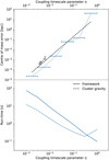 |
Fig. 7 Centre of mass error (top) and wall-clock run-time (bottom) as a function of timescale parameter, η, for a star cluster in a background galaxy potential. Centre-of-mass errors were computed between subsequent values of the coupling timescale, indicated by the ends of the error bars. The dashed black line indicates quadratic scaling of the centre of mass error with the coupling timescale. |
4.3 Combined model
Having demonstrated VENICE’s capabilities in small, controlled experiments, we now demonstrate its ability to build up complex simulations. In this section, we couple the models described above. We aim to simulate the dynamics of a star cluster in the potential of a galaxy, while following stellar mass loss due to stellar evolution. We set up the interactions between the cluster’s gravitational dynamics and stellar evolution models adaptively, in the same way as in Sect. 4.1.2, and the interaction between the cluster’s gravitational dynamics and the background potential as in Sect. 4.2.2. We used a stellar coupling timescale parameter (ηs) of 0.3, and a gravitational coupling timescale parameter (ηg) of 0.03.
1: procedure SETUP_BRIDGED_GRAVITY(gravity_cluster, stellar, gravity_galaxy, gravity_perturbers, ηs, ηg)
2: system = VENICE()
3: system.ADD_CODE(gravity_cluster)
4: system.ADD_CODE(stellar)
5: system.ADD_CODE(gravity_galaxy)
6: system.ADD_CODE(gravity_perturbers)
7: system.ADD_CHANNEL(1, 0, [“mass”])
8: ⊳ All gravity systems are coupled; stellar evolution only to cluster gravity
9: system.update_timescale[0][1] = lambda code1, code2, dt: ηs*code2.stellar_timesteps.MIN()
10: system.update_timescale[0][2] = lambda code1, code2, dt: ηg*MIN_FREEFALL_TIME(code1, code2)
11: system.update_timescale[0][3] = lambda code1, code2, dt: ηg*MIN_FREEFALL_TIME(code1, code2)
12: system.update_timescale[2][3] = lambda code1, code2, dt: ηg*MIN_FREEFALL_TIME(code1, code2)
13: ⊳ Galaxy and perturbers both kick cluster
14: system.kick[2][0] = dynamic_kick
15: system.kick[3][0] = dynamic_kick
16: ⊳ Galaxy kicks perturbers
17: system.kick[2][3] = dynamic_kick
18: return system
19: end procedure
In addition to combining the two models, we added two massive particles just outside the galactic disc, comparable in mass and location to the Large and Small Magellanic Clouds. We added these in their own gravity code, which is also coupled to the galaxy, and also perturbs the cluster (the cluster has no effect on other components). This separation into two codes allows us to couple the galaxy and these perturbers to the cluster on different timescales. In Pseudocode 5, we show how this system is set up.
For the cluster, we used the same 100-star, 10 pc Plummer sphere, with masses from a Kroupa IMF up to 8 M⊙, except that we gave three stars masses of 16, 30, and 50 M⊙. The cluster is initially on a circular orbit at 5 kpc from the galactic centre. The two perturbers have a mass of 1011 M⊙ each, and are initially at 50 and 60 kpc circular orbits, 180° and 90° ahead of the cluster, respectively. We evolved the system for 5 Gyr.
In Fig. 8, we show projections of this system on the galactic plane. The perturbers interact before having completed a full orbit, kicking the outer body inwards (towards the inner 10–15 kpc, still outside the cluster orbit) and kicking the inner body outwards. However, the cluster is still clearly perturbed; in runs without perturbers, the cluster disperses along a segment of a circle still 5 kpc in radius, while in runs with perturbers, stars are scattered throughout the galaxy. Overdensities remain in the inner 5 kpc, and around the final position of the perturber that was scattered inwards. A number of former cluster members appear to have become bound to this perturber.
In Fig. 9, we show the evolution of the star cluster by following the standard deviation of the cluster members’ polar co-ordinates through time.
If there are no perturbers, the radial standard deviation oscillates but remains below 1%, meaning that the stars remain close to their initial 5 kpc circular orbit. The azimuthal standard deviation increases mostly linearly, meaning that the cluster steadily disperses along its orbit. After 4 Gyr, there are steps in this standard deviation. This is likely a result from phase wrapping; if a considerable fraction of stars has angular co-ordinates around −π or π, the standard deviation may be biased. Some sections continue the initial linear trend, so the cluster continues to disperse. Both the radial and azimuthal standard deviations are smaller when stellar evolution is included. This is a counterintuitive result, because stellar evolution results in an increasingly unbound cluster that should promote dispersal into the galaxy.
When perturbers are added, the radial and azimuthal standard deviations increase and become less regular. After 3 Gyr, the radial standard deviation becomes of order unity, implying that the cluster is entirely scattered throughout the galaxy. The azimuthal standard deviation begins to deviate from the case without perturbers at about 2.5 Gyr. The standard deviation of a uniform distribution between [0, 2π] is ![Mathematical equation: $\[\frac{\pi}{\sqrt{3}} \approx 1.81\]$](/articles/aa/full_html/2024/11/aa48614-23/aa48614-23-eq39.png) , comparable to the value after 2.5 Gyr.
, comparable to the value after 2.5 Gyr.
In Fig. 10, we show the evolution time-steps of cluster gravity, perturber gravity, and stellar evolution codes through time, for the run with both perturbers and stellar evolution. The stellar time-steps drop below 1 yr during phases of rapid stellar evolution (as was seen before in Fig. 5), but can also be as large as ~100 Myr. The perturber and cluster time-steps are mostly constant before 3 Gyr (except when the stellar time-steps are small), reflecting that they mostly interact with the galaxy rather than each other. After 3 Gyr, these time-steps become much shorter, and this coincides with the moment the cluster’s radial standard deviation reaches unity. This confirms that the cluster’s disruption was due to interactions with a perturber.
5 Discussion
5.1 Future applications of the AMUSE implementation
Although almost any AMUSE simulation could be re-factored using VENICE, this does not necessarily yield a more efficient code or a clearer script. VENICE is especially useful in cases with many models or a wide (and dynamic) range of timescales. The adaptive coupling between gravity and stellar evolution could be worked out further; for example, by finding the ideal distribution of stars among multiple stellar evolution codes, depending on their lifetime distribution. This method could also be used for simulating the dynamics of smaller systems including planetary systems, such as the consequences of a planetary system once the parent star turns into a compact object, or the evolution of massive stellar triples (and higher-order multiples) in stellar clusters.
VENICE’s modular expandable nature can be used to gradually and hierarchically build up complex models, allowing both modules and interactions between modules to be characterised individually. A simple planet formation model where a single planet migrates and accretes from a static (gas, pebble, or planetesimal) disc can slowly be expanded to resemble, for example, the Bern model (see Fig. 2 in Emsenhuber et al. 2021, which has 14 physical modules), in which the effect of each module can be characterised individually. Codes can also be exchanged for more efficient or advanced alternatives, which should not affect interactions between other parts of the model that do not interact with that code.
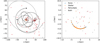 |
Fig. 8 Maps of the combined simulation projected on the galactic plane. The left panel shows a wide view, while the right panel is zoomed in on the centre. The dashed and dotted black lines show the trajectories of the two perturbers. Points show the positions at 5 Gyr of the cluster stars, where the colour indicates the model set-up (red and grey are with perturbers; orange and grey are with stellar evolution). |
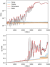 |
Fig. 9 Standard deviation of the distance to the galactic centre normalised to the mean distance (top) and of the azimuthal angle in the galactic plane (bottom) of the cluster members as a function of time. Colours indicate the model set-up (red and grey are with perturbers; orange and grey are with stellar evolution). |
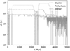 |
Fig. 10 Evolution timescales of different components of the combined model (including both stellar evolution and perturbers) through time. The dashed line indicates the cluster gravity, the dash-dotted line the perturber gravity, and the dotted line stellar evolution. |
5.2 Steps towards a differential equation solver
We have introduced VENICE, a coupling paradigm between numerical models. The designed method is also suitable for being applied to differential equation solvers. The main components that have not been developed yet are the integration of the individual operators (corresponding with the EVOLVE_MODEL functions) and the calculation of the coupling timescales, τij. Here, we sketch how such a method could be constructed.
The individual integration method could be practically any method with time-step control (e.g. Euler (forward or backward), (embedded) Runge–Kutta, or Bulirsch–Stoer), although a single method must be chosen for all operators. The coupling timescale of an operator pair will be the next time-step (predicted by the chosen method) for the differential equation where the right-hand side consists of just those two operators. If these operators are not coupled, this predicted timescale will be determined by the slowest of the two operators. This does not reflect their actual coupling timescale, which is still infinite. This was not an issue in the AMUSE implementation, where the internal evolution time-steps were decoupled from the coupling timescale.
The VENICE algorithm does not eliminate stiff parts of a set of differential equations, but decouples them from non-stiff parts. The integration method should therefore still be implicit in order to maintain stability. A (Bulirsch–Stoer-like) extrapolation method may be useful, because it may allow the slower operator of a fast pair to converge with few iterations, whereas an Euler or Runge–Kutta method will force the slow operator to take the same short time-steps as the fast operator.
A particular application for a VENICE-based differential equation solver would be a time-dependent chemical network integrator. This consists of many operators (chemical reactions) that operate on a range of timescales depending on reaction rates and chemical abundances.
6 Conclusion
We have introduced VENICE, an operator-splitting algorithm for multi-scale, multi-physics numerical problems, and demonstrated its working with examples from astrophysics. The simple examples show convergence with decreasing coupling times, although even with second-order (Strang) coupling this convergence is potentially only first-order, although second-order coupling typically results in smaller errors (even at a given wall-clock run-time). We have also shown that updating coupling timescales can result in appropriate adaptive time-stepping, and that gravitational BRIDGE interactions can be included as a coupling method. We then demonstrated how a complex model could be built up with VENICE.
The AMUSE implementation of VENICE can now be used as a framework for simulations, coupling a large number of numerical models on a wide range of timescales. We have also illustrated how VENICE can be used to construct a differential equation solver. This requires additional development, such as how to treat the timescales of individual evolution and coupling, and which integration method to use.
Acknowledgements
We thank Lourens Veen for the useful discussion on the differences and similarities between MUSCLE3 and VENICE, and Shuo Huang for early user feedback. MW is supported by NOVA under project number 10.2.5.12. The simulations in this work have been carried out on a work station equipped with an Intel Xeon W-2133 CPU, which consumes 140 W. At most, one out of six cores was used per simulation, putting power usage at 23 W. The amount of computer time used to develop and test VENICE and to produce the figures in this work were not recorded, but will be on the order of ~300 CPU hours. This puts the total power consumption at ~6 kWh. At 0.649 kWh/kg of CO2 emitted (Dutch norm for grey electricity), this comes to ~10 kg of CO2, comparable to a week of daily commutes.
References
- Aarseth, S. J. 1985, in Multiple Time Scales, 377 [Google Scholar]
- Allen, G., Benger, W., Dramlitsch, T., et al. 2001, in Euro-Par 2001 Parallel Processing: 7th International Euro-Par Conference Manchester, UK, August 28–31, 2001 Proceedings 7 (Springer), 817 [Google Scholar]
- Babur, O., Smilauer, V., Verhoeff, T., & van den Brand, M. 2015, in Procedia Computer Science Volume 51 Issue C, 1501 (Technische Universiteit Eindhoven), 1088 [Google Scholar]
- Borgdorff, J., Falcone, J.-L., Lorenz, E., et al. 2013, J. Parallel Distrib. Comput., 73, 465 [CrossRef] [Google Scholar]
- Bovy, J. 2015, ApJS, 216, 29 [NASA ADS] [CrossRef] [Google Scholar]
- Chopard, B., Borgdorff, J., & Hoekstra, A. 2014, Philos. Trans. Ser. A Math. Phys. Eng. Sci., 372 [Google Scholar]
- Christlieb, A. J., Liu, Y., & Xu, Z. 2015, J. Computat. Phys., 294, 224 [NASA ADS] [CrossRef] [Google Scholar]
- Einarsrud, K. E., Eick, I., Bai, W., et al. 2017, Appl. Math. Model., 44, 3 [CrossRef] [Google Scholar]
- Emsenhuber, A., Mordasini, C., Burn, R., et al. 2021, A&A, 656, A69 [NASA ADS] [CrossRef] [EDP Sciences] [Google Scholar]
- Fujii, M., Iwasawa, M., Funato, Y., & Makino, J. 2007, Publ. Astron. Soc. Japan, 59, 1095 [CrossRef] [Google Scholar]
- Goodale, T., Allen, G., Lanfermann, G., et al. 2003, in High Performance Computing for Computational Science – VECPAR 2002, ed. J. M. L. M. Palma, A. A. Sousa, J. Dongarra, & V. Hernández (Berlin, Heidelberg: Springer Berlin Heidelberg), 197 [CrossRef] [Google Scholar]
- Huang, S., Portegies Zwart, S., & Wilhelm, M. J. C. 2024, A&A, 689, A338 [NASA ADS] [CrossRef] [EDP Sciences] [Google Scholar]
- Jänes, J., Pelupessy, I., & Portegies Zwart, S. 2014, A&A, 570, A20 [NASA ADS] [CrossRef] [EDP Sciences] [Google Scholar]
- Jia, H., & Li, K. 2011, Math. Comput. Model., 53, 387 [CrossRef] [Google Scholar]
- Kroupa, P. 2001, MNRAS, 322, 231 [NASA ADS] [CrossRef] [Google Scholar]
- McMillan, S., Portegies Zwart, S., van Elteren, A., & Whitehead, A. 2012, in Advances in Computational Astrophysics: Methods, Tools, and Outcome, eds. R. Capuzzo-Dolcetta, M. Limongi, & A. Tornambè, Astronomical Society of the Pacific Conference Series, 453, 129 [NASA ADS] [Google Scholar]
- McMillan, S. L. W. 1986, in The Use of Supercomputers in Stellar Dynamics, 267, eds. P. Hut, & S. L. W. McMillan, 156 [NASA ADS] [CrossRef] [Google Scholar]
- Miller, R. H. 1964, ApJ, 140, 250 [NASA ADS] [CrossRef] [Google Scholar]
- Miyamoto, M., & Nagai, R. 1975, Publ. Astron. Soc. Japan, 27, 533 [Google Scholar]
- Navarro, J. F., Frenk, C. S., & White, S. D. M. 1996, ApJ, 462, 563 [Google Scholar]
- Pelupessy, F. I., & Portegies Zwart, S. 2012, MNRAS, 420, 1503 [NASA ADS] [CrossRef] [Google Scholar]
- Pelupessy, F. I., Jänes, J., & Portegies Zwart, S. 2012, New Astron., 17, 711 [Google Scholar]
- Pelupessy, F. I., van Elteren, A., de Vries, N., et al. 2013, A&A, 557, A84 [NASA ADS] [CrossRef] [EDP Sciences] [Google Scholar]
- Peters, B., Baniasadi, M., Baniasadi, M., et al. 2018, arXiv e-prints [arXiv:1808.08028] [Google Scholar]
- Portegies Zwart, S. 2018, Science, 361, 979 [NASA ADS] [CrossRef] [Google Scholar]
- Portegies Zwart, S. F., & Verbunt, F. 1996, A&A, 309, 179 [NASA ADS] [Google Scholar]
- Portegies Zwart, S., McMillan, S., Harfst, S., et al. 2009, New Astron., 14, 369 [Google Scholar]
- Portegies Zwart, S., McMillan, S. L. W., van Elteren, E., Pelupessy, I., & de Vries, N. 2013, Comput. Phys. Commun., 184, 456 [Google Scholar]
- Portegies Zwart, S., Pelupessy, I., Martínez-Barbosa, C., van Elteren, A., & McMillan, S. 2020a, Commun. Nonlinear Sci. Numer. Simul., 85, 105240 [Google Scholar]
- Portegies Zwart, S., Pelupessy, I., Martínez-Barbosa, C., van Elteren, A., & McMillan, S. 2020b, Commun. Nonlinear Sci. Numer. Simul., 85, 105240 [Google Scholar]
- Rin, R., Tomin, P., Garipov, T., Voskov, D., & Tchelepi, H., eds. 2017, SPE Reservoir Simulation Conference, Vol. Day 3 Wed, February 22, 2017, General Implicit Coupling Framework for Multi-Physics Problems, eds. R. Rin, P. Tomin, T. Garipov, D. Voskov, & H. Tchelepi, D031S012R001 [Google Scholar]
- Strang, G. 1968, SIAM J. Numer. Anal., 5, 506 [CrossRef] [MathSciNet] [Google Scholar]
- Terlevich, E. 1987, MNRAS, 224, 193 [NASA ADS] [CrossRef] [Google Scholar]
- Toonen, S., Nelemans, G., & Portegies Zwart, S. 2012, A&A, 546, A70 [NASA ADS] [CrossRef] [EDP Sciences] [Google Scholar]
- van Elteren, A., Portegies Zwart, S., Pelupessy, I., Cai, M. X., & McMillan, S. L. W. 2019, A&A, 624, A120 [NASA ADS] [CrossRef] [EDP Sciences] [Google Scholar]
- Veen, L. E., & Hoekstra, A. G. 2020, in Computational Science – ICCS 2020, eds. V. V. Krzhizhanovskaya, G. Závodszky, M. H. Lees, et al. (Cham: Springer International Publishing), 425 [CrossRef] [Google Scholar]
- Verlet, L. 1967, Phys. Rev., 159, 98 [CrossRef] [Google Scholar]
- Wielen, R. 1967, Veroeffentlich. Astron. Rechen-Inst. Heidelberg, 19, 1 [NASA ADS] [Google Scholar]
- Xianmeng, W., Mingyu, W., Xiao, H., et al. 2021, Veroeffentlichungen Simulation, 97, 687 [CrossRef] [Google Scholar]
Note the difference between timescales and time-steps: timescales are a derived physical quantity of a system, while time-steps are a property of the algorithm, external to the physics of the system.
Note the implicit assumption here that the BRIDGE timescale is the same as the previously defined coupling timescales, τij.
The increase in the run-time is due to the gravity model running twice as long.
If the system is evolved for multiple time-steps, Δt, there may be two sequential half-time-steps, e.g.: ![Mathematical equation: $\[e^{\hat{L}_1 \Delta t / 2} e^{\hat{L}_2 \Delta t}\left(e^{\hat{L}_1 \Delta t / 2} e^{\hat{L}_1 \Delta t / 2}\right) e^{\hat{L}_2 \Delta t} e^{\hat{L}_1 \Delta t / 2}\]$](/articles/aa/full_html/2024/11/aa48614-23/aa48614-23-eq40.png) . These could be combined in a single evolution step, with a potential for faster evolution, but for larger systems there could be operators in between, and the coupling timescales may change in between. Therefore, such recombination is not possible.
. These could be combined in a single evolution step, with a potential for faster evolution, but for larger systems there could be operators in between, and the coupling timescales may change in between. Therefore, such recombination is not possible.
All Figures
|
Fig. 1 Timescale matrix for a VENICE implementation. Left: representation of the coupling timescale matrix, τ, of an operator set as an undirected, weighted graph. Edges are labelled with the coupling timescale; some edges between triangulated nodes share labels for clarity. The coupling timescale between unconnected nodes is ∞. Right: tree representation of the recursive splitting of connected components, for the system on the left. Dotted lines denote skipped layers of nodes with a single parent and child node. |
| In the text | |
|
Fig. 2 Convergence and performance of a gravitational dynamics model and a stellar evolution one, coupled at a constant timescale. The top panels and the bottom left panel show three views of the median position error, coupling timescale, and wall-clock run-time as functions of each other. The bottom right panel shows the time evolution of the median position error in all runs. The dashed black lines in the top left plot show linear and quadratic scalings of the error with the timescale. |
| In the text | |
|
Fig. 3 Convergence and performance of a gravitational dynamics and stellar evolution model coupled at a constant timescale, with reversed operators. We show, as a function of the coupling timescale, the median position error (top) and wall-clock run-time (bottom). The dashed black lines in the top plot show linear and quadratic scalings of the error with the timescale. |
| In the text | |
|
Fig. 4 Convergence and performance of a gravitational dynamics and a stellar evolution model coupled at an adaptive timescale. We show, as a function of the timescale parameter, η, the median position error (top) and wall-clock run-time (bottom). The median position error was computed for two subsequent values of the coupling timescale, indicated by the endpoints of the error bars. The dashed black lines in the top plot show linear and quadratic scalings of the error with the timescale. |
| In the text | |
|
Fig. 5 Evolution of the dynamic coupling time-scales. Top: dynamic coupling timescale between the gravitational dynamics and stellar evolution models as a function of time, for a number of timescale parameters, η. Bottom: the stellar type through time of a 50 M⊙ star, which is the most massive one in the system of the top panel. |
| In the text | |
|
Fig. 6 Centre of mass error (top) and wall-clock run-time (bottom) as a function of constant coupling timescale, for a star cluster in a background galaxy potential. Centre of mass errors were computed between subsequent values of the coupling timescale, indicated by the ends of the error bars. The dashed black line indicates quadratic scaling of the centre of mass error with the coupling timescale. |
| In the text | |
|
Fig. 7 Centre of mass error (top) and wall-clock run-time (bottom) as a function of timescale parameter, η, for a star cluster in a background galaxy potential. Centre-of-mass errors were computed between subsequent values of the coupling timescale, indicated by the ends of the error bars. The dashed black line indicates quadratic scaling of the centre of mass error with the coupling timescale. |
| In the text | |
|
Fig. 8 Maps of the combined simulation projected on the galactic plane. The left panel shows a wide view, while the right panel is zoomed in on the centre. The dashed and dotted black lines show the trajectories of the two perturbers. Points show the positions at 5 Gyr of the cluster stars, where the colour indicates the model set-up (red and grey are with perturbers; orange and grey are with stellar evolution). |
| In the text | |
|
Fig. 9 Standard deviation of the distance to the galactic centre normalised to the mean distance (top) and of the azimuthal angle in the galactic plane (bottom) of the cluster members as a function of time. Colours indicate the model set-up (red and grey are with perturbers; orange and grey are with stellar evolution). |
| In the text | |
|
Fig. 10 Evolution timescales of different components of the combined model (including both stellar evolution and perturbers) through time. The dashed line indicates the cluster gravity, the dash-dotted line the perturber gravity, and the dotted line stellar evolution. |
| In the text | |
Current usage metrics show cumulative count of Article Views (full-text article views including HTML views, PDF and ePub downloads, according to the available data) and Abstracts Views on Vision4Press platform.
Data correspond to usage on the plateform after 2015. The current usage metrics is available 48-96 hours after online publication and is updated daily on week days.
Initial download of the metrics may take a while.