| Issue |
A&A
Volume 684, April 2024
|
|
|---|---|---|
| Article Number | A196 | |
| Number of page(s) | 9 | |
| Section | Extragalactic astronomy | |
| DOI | https://doi.org/10.1051/0004-6361/202348351 | |
| Published online | 24 April 2024 | |
Noema formIng Cluster survEy (NICE): Discovery of a starbursting galaxy group with a radio-luminous core at z = 3.95
1
School of Astronomy and Space Science, Nanjing University, Nanjing 210093, PR China
e-mail: This email address is being protected from spambots. You need JavaScript enabled to view it.
2
Key Laboratory of Modern Astronomy and Astrophysics (Nanjing University), Ministry of Education, Nanjing 210093, PR China
3
AIM, CEA, CNRS, Université Paris-Saclay, Université Paris Diderot, Sorbonne Paris Cité, 91191 Gif-sur-Yvette, France
4
IRAM, 300 rue de la piscine, 38406 Saint-Martin-d’Hères, France
5
Cosmic Dawn Center (DAWN), Jagtvej 128, 2200 Copenhagen N, Denmark
6
DTU-Space, Technical University of Denmark, Elektrovej 327, 2800 Kgs. Lyngby, Denmark
7
Max-Planck-Institut für Extraterrestrische Physik (MPE), Giessenbachstrasse 1, 85748 Garching, Germany
8
Purple Mountain Observatory, Chinese Academy of Sciences, 10 Yuanhua Road, Nanjing 210023, PR China
9
Niels Bohr Institute, University of Copenhagen, Jagtvej 128, 2200 Copenhagen N, Denmark
10
Instituto de Astrofísica de Canarias, C. Vía Láctea, s/n, 38205 La Laguna, Tenerife, Spain
11
Universidad de La Laguna, Dpto. Astrofísica, 38206 La Laguna, Tenerife, Spain
12
European Southern Observatory, Karl-Schwarzschild-Str. 2, 85748 Garching bei Munchen, Germany
13
Steward Observatory, University of Arizona, 933 N. Cherry Avenue, Tucson, AZ 85721, USA
14
INAF – Osservatorio Astronomico di Brera, Via Brera 28, 20121, Milano, Italy & Via Bianchi 46, 23807 Merate, Italy
15
Department of Astronomy, University of Geneva, Chemin Pegasi 51, 1290 Versoix, Switzerland
16
Instituto de Física, Pontificia Universidad Católica de Valparaíso, Casilla 4059, Valparaíso, Chile
17
INAF – Osservatorio Astronomico di Trieste, Via Tiepolo 11, 34131 Trieste, Italy
18
IFPU – Institute for Fundamental Physics of the Universe, Via Beirut 2, 34014 Trieste, Italy
19
Department of Physics, University of Helsinki, Gustaf Hällströmin katu 2, 00014 Helsinki, Finland
20
Department of Physics & Astronomy, University of California Los Angeles, 430 Portola Plaza, Los Angeles, CA 90095, USA
21
Chinese Academy of Sciences South America Center for Astronomy, National Astronomical Observatories, CAS, Beijing 100101, PR China
Received:
23
October
2023
Accepted:
7
February
2024
Abstract
The study of distant galaxy groups and clusters at the peak epoch of star formation is limited by the lack of a statistically and homogeneously selected and spectroscopically confirmed sample. Recent discoveries of concentrated starburst activities in cluster cores have opened a new window to hunt for these structures based on their integrated IR luminosities. Here, we carry out a large NOEMA (NOrthern Extended Millimeter Array) program targeting a statistical sample of infrared-luminous sources associated with overdensities of massive galaxies at z > 2, the Noema formIng Cluster survEy (NICE). We present the first result from the ongoing NICE survey, a compact group at z = 3.95 in the Lockman Hole field (LH-SBC3), confirmed via four massive (M⋆ ≳ 1010.5 M⊙) galaxies detected in the CO(4–3) and [CI](1–0) lines. The four CO-detected members of LH-SBC3 are distributed over a 180 kpc physical scale and the entire structure has an estimated halo mass of ∼1013 M⊙ and total star formation rate of ∼4000 M⊙ yr−1. In addition, the most massive galaxy hosts a radio-loud active galactic nucleus with L1.4 GHz, rest = 3.0 × 1025 W Hz−1. The discovery of LH-SBC3 demonstrates the feasibility of our method to efficiently identify high-z compact groups or cluster cores undergoing formation. The existence of these starbursting cluster cores up to z ∼ 4 provides critical insights into the mass assembly history of the central massive galaxies in clusters.
Key words: galaxies: clusters: general / galaxies: evolution / galaxies: high-redshift / submillimeter: galaxies
© The Authors 2024
 Open Access article, published by EDP Sciences, under the terms of the Creative Commons Attribution License (https://creativecommons.org/licenses/by/4.0), which permits unrestricted use, distribution, and reproduction in any medium, provided the original work is properly cited.
This article is published in open access under the Subscribe to Open model. This email address is being protected from spambots. You need JavaScript enabled to view it. to support open access publication.
1. Introduction
Galaxy groups and clusters at cosmic noon and earlier are key to understanding the physical processes that lead to the emergence of the peak in the cosmic star formation history (Madau & Dickinson 2014; Overzier 2016). They are the progenitors of the galaxy clusters in the local Universe, however, they are still actively forming stars (Kravtsov & Borgani 2012). Hence, they are ideal laboratories to study the formation and quenching of massive galaxies. Meanwhile, these high-z galaxy groups and clusters reside in massive halos and are expected to accrete cold gas effectively, fueling star formation in the structures, namely, as per cold accretion theory (Dekel et al. 2009; Daddi et al. 2021). This is contrast to local galaxy clusters where gas streams are disrupted or heated when entering the hot dark matter halos (Kereš et al. 2005). Furthermore, the statistics of the number of dark matter halos that host them as a function of redshift and total mass can be used to constrain cosmological parameters and test structure formation theories (see Allen et al. 2011 and references therein). However, observational constraints remain scarce.
Identifying star-forming structures is not straightforward. Radio galaxies have been used as tracers of proto-clusters (e.g., Miley et al. 2006; Daddi et al. 2009; Wylezalek et al. 2013; Shen et al. 2021), as they tend to reside in massive dark matter halos. However, they do not always trace the structures concurrently undergoing active star formation (Cooke et al. 2015). Quite a few Mpc-scale overdensities of emission line galaxies have been discovered in the last two decades (e.g., Pentericci et al. 2000; Kurk et al. 2000; Steidel et al. 2005; Koyama et al. 2013; Toshikawa et al. 2018; Lemaux et al. 2018), thanks to the spectroscopy and narrowband imaging of 10m class telescopes. Additionally, massive overdensities are revealed by strong intergalactic Lyα absorption systems in QSO spectra (Cai et al. 2017) and some other tracers including; for instance, Lyman α blobs and QSOs are also used (see Overzier 2016). These extended structures host multiple dark matter halos that may today end up in a single cluster (Chiang et al. 2013; Muldrew et al. 2015). However, it would be complicated to track down the formation history of the ensemble in simulations and test theories directly, as opposed to single dark matter halos. In this work, we focus on infrared luminous galaxy groups and clusters hosting the most massive halos at cosmic noon and earlier.
Submillimeter observations have achieved success in searching for these structures (e.g., Capak et al. 2011; Walter et al. 2012; Casey 2016; Wang et al. 2016a; Oteo et al. 2018; Miller et al. 2018; Zhou et al. 2020), but the samples remain limited and heterogeneous. Besides, selections via overdensities of submillimeter galaxies alone suffer from projection effects (Chen et al. 2023). Efficient searches require additional constraints on redshift. This has motivated the Noema formIng Cluster survEy (NICE), which systematically searches for the massive halos in formation at 2 ≲ z ≲ 4. The NICE survey selects overdensities of infrared luminous and massive galaxies based on deep far-infrared (FIR) and mid-infrared (MIR) priors from Herschel/SPIRE and Spitzer/IRAC observations, and then spectroscopically confirms them with the gas emission lines detected by NOEMA.
This paper presents an overview of the NICE survey. Among the first structures confirmed in the NICE survey, this paper also highlights the most distant one, LH-SBC3, which is a starbursting galaxy group with a radio-luminous core at z = 3.95. Throughout this paper, we adopt a spatially flat ΛCDM cosmological model with H0 = 70 km s−1 Mpc−1, Ωm = 0.3, and ΩΛ = 0.7. We assume a Salpeter (1955) initial mass function (IMF) with a conversion factor of 1.7 from the Chabrier (2003) IMF when necessary. All magnitudes are quoted in the AB system (Oke & Gunn 1983).
2. Noema formIng Cluster survEy (NICE)
2.1. Survey overview
The NICE survey is a 159-h NOEMA large program (PIs: E. Daddi and T. Wang, proposal ID:M21AA) targeting 48 galaxy overdensities selected from five fields, namely, Lockman Hole, Elais-N1, Boötes, XMM-LSS, and COSMOS. Altogether, 25 candidates in the southern sky are complemented by the 40-h ALMA Cycle8 observations (PI: E.Daddi, project ID: 2021.1.00815.S) in the ECDFS, COSMOS, and XMM-LSS fields, overlapping with 4 candidates in the NOEMA observations.
2.2. NICE candidates selection criteria
The NICE survey targets starbursting massive galaxy groups and clusters at 2 ≲ z ≲ 4. We select overdensities of high-z massive galaxies traced by red IRAC detections in association with SPIRE-350 μm peakers that show intense star formation. In the following, we concisely describe the selection criteria, a detailed introduction will be presented in Zhou et al. (in prep.).
2.2.1. IRAC selected overdensities
We used an IRAC color cut as shown in Eq. (1) to select massive galaxies at z > 2. This selection criterion is based on the 1.6 μm bump in the SEDs of galaxies resulting from a minimum in the opacity of the H− ion in the atmospheres of cool stars (John 1988). This method has proved to be efficient in isolating high-z galaxies (Papovich 2008; Galametz et al. 2012) and we chose a redder color to select galaxies at higher redshifts. Meanwhile, we constrained the [4.5] mag to select massive galaxies, while excluding the contamination from stars. In Fig. 1, we show the distribution of the galaxies compiled in the COSMOS2020 catalogue (Weaver et al. 2022) and find that most of the massive star-forming galaxies (SFGs) meet our selection criterion:
![Mathematical equation: $$ \begin{aligned}&{[3.6]-[4.5]} > {0.1} ; \nonumber \\&{20}<{[4.5]} < { 23}. \end{aligned} $$](/articles/aa/full_html/2024/04/aa48351-23/aa48351-23-eq1.gif) (1)
(1)
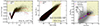 |
Fig. 1. NICE candidates selection criteria. Left: IRAC color to constrain the redshift to be 2 ≲ z ≲ 4. Data points are UVJ color selected massive SFGs from COSMOS2020 (Weaver et al. 2022). Solid and dashed red curves show the median and the lower limit of 90% of the galaxies. The yellow shade shows the selection criterion. Middle: IRAC2 magnitude to choose galaxies more massive than 1010 M⊙. Data points are UVJ color selected SFGs at 2 < zphot < 4 from COSMOS2020. The red curves and the yellow shade are the same as in the left panel. Right: Herschel/SPIRE colors to select starbursting structures at 2 ≲ z ≲ 4. Grey dots are the Herschel detections in all the NICE survey fields, while the black dots meet the selection criteria in Eq. (2). The blue, red, and magenta curves show the trend of main sequence galaxies, starbursts and SMGs and the circles are marked by the redshifts accordingly. The starbursting proto-cluster at z = 2.51, CL-J1001, is presented as an orange star. See details in Sect. 2.2.2. The inserted histogram displays the distribution of 500 μm fluxes. |
We used the Nth closest neighbour,  , where dN is the distance to the Nth closest galaxy, as the density estimator. For each field, we created a grid with cell sizes of 3″ and calculate ΣN at each cell to construct the surface density map of the color-selected sources. We then compute the mean and standard deviation of the surface density across each field. Regions above 5σ are defined as overdensities. We used both Σ5 and Σ10 and chose targets that satisfied either of those. Figure 2 (left) shows an example of the Σ10 map centred on LH-SBC3, which is so far the most distant galaxy group identified in the NICE survey.
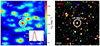 |
Fig. 2. LH-SBC3 selected following the method in Sect. 2.2. Left: smoothed Σ10 map of the red IRAC priors (Eq. (1)) over the 25′×25′ area around LH-SBC3. The construction of the map is described in Sect. 2.2.1. The inserted histogram is the distribution of Σ10 (black histogram) and the Gaussian fit (red dashed curve). The red arrow indicates the peak Σ10 value of LH-SBC3. Right: Herschel/SPIRE composite color image of the same area. The R, G, and B channels correspond to 500 μm, 350 μm, and 250 μm, respectively. The white circles in both figures have a radius of 2′. |
2.2.2. Herschel selected 350 μm peakers
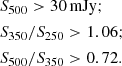
The Herschel/SPIRE observations typically have beam sizes of 20″–36″, consistent with spatial scales of massive halos at 2 ≲ z ≲ 4. Therefore, in addition to the IRAC color selection, we verify the collective star formation activities in massive halos with SPIRE colors. The SPIRE color evolution with redshifts for three different types of galaxy SEDs is shown in Fig. 1 (right). The main sequence and starburst SED templates are based on stacking (Magdis et al. 2012). The template for ALESS z ∼ 2 submillimeter galaxies (SMGs) is taken from da Cunha et al. (2015). Due to the different PSF sizes of the SPIRE bands, the fluxes at longer wavelengths include more sources. As a result, the observed colors of the galaxy clusters/groups are redder than those predicted by individual galaxies. This is corrected based on the comparison between SPIRE colors of the starbursting clusters at z = 2.51, CL-J1001 (Wang et al. 2016b), and individual galaxies at similar redshifts, which leads to our final sample selection criterion of 2 ≲ z ≲ 4 candidates as in Eq. (2). We also require sources to be IR bright with S500 > 30 mJy (above 5σ confusion noise), which corresponds to LIR ∼ 1013 L⊙ at z = 2.5:
 (2)
(2)
2.3. NOEMA observations
The NOEMA observations were conducted in band 1 with two setups. The first setup covers 87.7–95.7 GHz and 103.2–111.2 GHz or 80.0–88.0 GHz and 95.5–103.5 GHz depending on the estimated redshift of the structures, while the second setup is subsequently arranged on the basis of the detected lines from the first setup, meant to optimize the detections. In general, the observations allow detections of CO(3–2) if they fall at z ∼ 1.9–3.4, or CO(4–3) if they are at z ∼ 2.9–4.8. The spectra reach a typical rms sensitivity of ∼130 μJy beam−1 over 500 km s−1, and the continuum reaches ∼14.5 μJy beam−1 over the bandwidth of 16 GHz per polarization. Configurations C and D were adopted to spatially separate the different member galaxies while conserving their total fluxes and then the spatial resolution is θ ∼ 2″. The starbursting massive galaxy groups/clusters selected by the NICE survey are aptly covered by the half-power beam width (HPBW ∼ 50″).
2.4. NOEMA data reduction and source extraction
The NOEMA data were calibrated and reduced using GILDAS1. We produced uv tables following the standard NOEMA data reduction with GILDAS CLIC package2, which includes bandpass, phase, amplitude and flux scale calibration, and data flagging. We then made dirty and clean images using GILDAS MAPPING go uvmap and go clean tasks; meanwhile, we extracted spectra for multiple sources simultaneously in the uv plane using the run uv_fit task. This GILDAS uv_fit task can model analytical source models in the image plane and convert the emission to the Fourier space then directly fit the observed visibilities. This is similar to the CASA uvmodelfit, but the latter cannot fit multiple sources simultaneously. The phase centres were set as the coordinates of the NICE candidates, namely, the coordinates of the corresponding SPIRE-350 μm peakers. Primary beam attenuation correction was estimated for each source at their corresponding positions in the image, based on the GILDAS MAPPING go primary task with the correction factors ranging from 1.01 to 1.22, and the corrections were applied to the line and continuum measurements. Natural weighting was adopted in the imaging procedures to maximize the sensitivity and a cleaning threshold of 2.5σ is used when running the GILDAS MAPPINGgo clean task. We first extracted the spectra of continuum detections. If a source is spatially resolved, we use a Gaussian model to fit the uvdata and then extract the spectra. The unresolved sources were extracted by fitting point sources. The same procedure is also performed at the IRAC position of each cluster member candidate. After combining the spectra from two observation setups, we run the line-searching algorithm as in Coogan et al. (2019) over each 1D spectrum. We first measured the line-free continuum using a noise-weighted fit, assuming a slope of 3.7 in frequency and obtain the continuum flux. We then subtracted the continuum from the spectra and use MPFIT3 to fit the lines with Gaussians. We obtained the redshift from the first line considering the photometric of the galaxies and then fixed the redshift and measured the second.
3. LH-SBC3: A galaxy group at z = 3.95
LH-SBC3 is a galaxy group at z = 3.95 in the Lockman Hole field. Among the first NICE structures that are spectroscopically confirmed, it is also the most distant one. We present it here as a highlight.
LH-SBC3 consists of four members detected with CO(4–3), LH-SBC3.a, b, c, and d (as shown in Fig. 3). The two brightest ones, LH-SBC3.a and b, also show [CI](1–0) with which we robustly confirm their redshifts. The line and continuum detections are listed in Table 1. LH-SBC3.a and d are two spatially resolved peaks in the continuum at 3 mm. They are around 3″ apart, larger than the typical size of a massive star-forming galaxy at z ∼ 4. We will also show in Sect. 3.2 that LH-SBC3.d has marginal detection at 150 MHz 3″ from LH-SBC3.a. Two more sources have emission lines detected at fobs ∼ 108 GHz. Based on their photometric redshifts, they are most likely at z ∼ 2.2 and the lines correspond to CO(3–2). They could also be at z ∼ 3.2 if the lines are CO(4–3). In either case, they may be part of a foreground structure. The spectra of these two galaxies are shown in Fig. A.1.
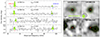 |
Fig. 3. The four members of LH-SBC3 spectroscopically confirmed by NOEMA. Left: NOEMA spectra of four confirmed cluster members. The channel width of the spectra is rebinned to be ∼150 km s−1. The detected lines are highlighted in yellow. CO(4–3) and [CI](1–0) frequencies are marked by vertical bars in red and blue, respectively. Right: 3 mm continuum images of the four members overlaid by CO(4–3) intensity contours in yellow. The red circles denote the positions of the galaxies determined by the flux peak of the 3 mm continuum. The CO(4–3) intensity contours start at 1σ (equivalent to ∼56 mJy km−1 beam−1) in steps of 1σ. Beams of the 3 mm and CO(4–3) intensity maps are shown in the second panel as black-hatched and yellow patterns corresponding to 3.43″ × 3.60″and 2.37″ × 2.02″, respectively. |
Line and continuum detections of LH-SBC3 members.
LH-SBC3 was selected to have a 7σ excess in Σ10 when searching in the entire Lockman Hole field (Fig. 2-Left). It contains six IRAC priors as selected by Eq. (1) within a radius of 25″ (r ∼ 180 pkpc, Fig. 4). The four NOEMA detections were not selected as priors because they are intrinsically faint (high dust obscuration) at the IRAC wavelength and tend to be blended in this crowded region, which increases the uncertainty of their photometry, and IRAC colors. We supplement the existing images with additional H, K observations from CFHT (PI: T. Wang) and use the deeper NIR images for source extraction. This is to avoid the dilution of these optically faint IRAC priors in the detection image. Finally, we confirmed that LH-SBC3.b and LH-SBC3.c should have been selected while LH-SBC3.a and LH-SBC3.d are too close to de-blend and hence missed. Besides, the spatial distribution of galaxies with photometric redshift intervals consistent with z ∼ 3.95 shows an apparent excess of massive galaxies centred on LH-SBC3 (Fig. 4), which reinforces the existence of an overdensed structure here.
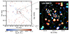 |
Fig. 4. Left: spatial distribution of galaxies with photometric redshift intervals consistent with z = 3.95. The dashed box denotes the 1′ × 1′(∼2 cMpc × 2 cMpc) region of the galaxy overdensity, LH-SBC3. The dots are color-coded by their stellar masses. Right: zoom-in RGB image (red: IRAC2; green: K; blue: i) of LH-SBC3. The white solid contours denote the 3 mm continuum, starting at 2σ in steps of 1σ. The four CO-confirmed members are labelled with their IDs. Note: LH-SBC3.a and d are very close. The cyan dashed circles are the IRAC-color selected priors. The priors labelled with a question mark could come from another structure at z = 3.25 or z = 2.19, see discussion in Sect. 3. The dotted white contours show 500 μm flux at 20, 40, 60 mJy beam−1 levels. |
LH-SBC3 shows strong emission in the FIR (Fig. 2, right panel) indicating intensive star formation. After deblending the foreground sources from the SPIRE images following Jin et al. (2018, also see Liu et al. 2018), we obtained the SPIRE fluxes of the structure to be S250 = 54.6 ± 5.3 mJy, S350 = 73.8 ± 6.7 mJy, and S500 = 69.3 ± 8.4 mJy. In Fig. 5, we find that the total flux of the four members at 3 mm is well fitted by an optically thin dust model with MERCURIUS4 as in Witstok et al. (2022). Therefore we rule out the line-of-sight interlopers contributing to the Herschel/SPIRE fluxes.
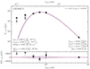 |
Fig. 5. FIR SED of LH-SBC3. Line-of-sight contamination to the SPIRE fluxes is subtracted using the deblending procedures in Jin et al. (2018). The 3 mm flux is well fitted by an optically thin dust model (Witstok et al. 2022). |
3.1. Properties of LH-SBC3
We fit the optical to mid-infrared SEDs using FAST++5, CIGALE (Boquien et al. 2019), and BAGPIPES (Carnall et al. 2018) to derive the stellar masses (M⋆). All codes give consistent results. We assume delayed star formation history and a Calzetti et al. (2000) attenuation curve in the fitting. If assuming constant star formation history, the derived masses would be no more than 0.3 dex lower. Three of the four members are massive, with M⋆ > 1010.5 M⊙ (Table 2).
Physical properties of LH-SBC3 members.
We calculated the star formation rate (SFR) with three methods. First, we fitted the mid-IR to 3 mm fluxes with CIGALE to get the SFRs. For LH-SBC3.a and LH-SBC3.b, we included the deblended SPIRE fluxes following the procedure described in Jin et al. (2018). Second, we scaled the 3 mm fluxes of the individual members with the total flux of the entire structure that can be used to derive the total SFR of the group; we confirm in Fig. 5 that the deblended SPIRE fluxes and 3 mm flux of LH-SBC3 match the dust emission model well. Third, we used the CO(4–3)–LIR scaling relation (Liu et al. 2015), which considers dense molecular gas emitting at high-J as good tracers of star formation. These three methods give consistent results overall. Hereafter, we use the scaled SFRs as in the second method.
The four CO detected members are concentrated in an area of r < 0.2 pMpc, the typical size of a proto-cluster core at z ∼ 4 (Chiang et al. 2017) and show tentative velocity dispersion within 500 km s−1 of the average redshift comparable to the virial velocity (e.g., Daddi et al. 2021), then LH-SBC3 is consistent with being a single massive halo. We estimated the halo masses (Mhalo) of LH-SBC3 with two different methods. First, we adopted the Mhalo − M⋆ scaling relation in Behroozi et al. (2013), with the most massive member of LH-SBC3 giving an upper limit of Mhalo ∼ 1013.2 M⊙. Second, we first derived the total stellar mass of the galaxies with stellar masses of M⋆ > 1010.5 M⊙ in LH-SBC3 to be 1011.37 M⊙ if we count only the CO detected members, or 1011.68 M⊙ if we include all the galaxies with zphot ∼ 3.95, as shown in Fig. 4. We then extrapolated a total stellar mass down to 107 M⊙ assuming the stellar mass function of field galaxies from Muzzin et al. (2013) at 3 ≤ z < 4, and obtain 1011.41 − 1011.72 M⊙. Finally, we adopted the scaling relation between total stellar and halo mass derived from z ∼ 1 clusters with halo masses in the range of 0.6–16 × 1014 M⊙ (van der Burg et al. 2014) and yielded a halo mass of Mhalo ∼ 1012.7 − 1013.2 M⊙.
We further measured the halo mass-normalized integrated SFR (ΣSFR/Mhalo) of LH-SBC3. Assuming that the star formation in the structure is dominated by the four NOEMA detected members, we obtained ΣSFR/Mhalo ∼ 2 − 10 × 10−10 yr−1, around 2 dex higher than the clusters at z = 1–2 (Alberts et al. 2016). Compared to clusters at lower redshifts, we find that ΣSFR/Mhalo rises rapidly with redshift, as predicted by Alberts et al. (2014; see a discussion in Popesso et al. 2015; Alberts & Noble 2022). This indicates vigorous star formation in the structures in the early Universe. We speculate that LH-SBC3 is still in the growing phase and will evolve into a transitioning phase, similarly to the case of CL J1001 at z ∼ 2.5 (Wang et al. 2016b).
In Fig. 6, we compare member galaxies of LH-SBC3 with those in two other starbursting proto-clusters at a z ∼ 4 Dense Red Core (DRC, Oteo et al. 2018), and SPT2349-56 (Miller et al. 2018). The LH-SBC3 member galaxies generally fall within the scatter shown by DRC and SPT2349-56. The two strongest CO emitters, LH-SBC3.a and LH-SBC3.b are massive and starbursting.
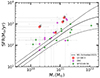 |
Fig. 6. Position of the LH-SBC3 member galaxies (red circles) with respect to the star-forming main sequence at z = 4 (Schreiber et al. 2015). Galaxies in the Dense Red Core (DRC, z = 4; Oteo et al. 2018; Long et al. 2020) and SPT2349-56 (z = 4.3, Miller et al. 2018; Hill et al. 2022) are shown as magenta and green circles, respectively. |
3.2. A radio-luminous core
The most massive of the four CO-confirmed members, LH-SBC3.a, shows strong radio emission at 150 MHz, S150 MHz = 1519 μJy. Comparing the fluxes in the high (0.3″) and low (6″) spatial resolution images (Sweijen et al. 2022; Tasse et al. 2021), we find that all the radio emission originates from the core of this galaxy (Fig. 7). This galaxy is also detected at 324.5 MHz (corresponding to 1.6 GHz in the rest-frame) by the VLA, with S324.5 MHz = 888 μJy (Owen et al. 2009). This gives a radio spectral index of α = −0.7 and we derive a radio luminosity of L1.4 GHz, rest = 3.0 × 1025 W Hz−1. We find that the radio luminosity is about five times higher than expected from star formation (Delhaize et al. 2017; Delvecchio et al. 2021), indicating the existence of a radio AGN. Still, it shows no signs of other active galactic nuclei (AGNs) in diagnostics available (optical, MIR, or X-ray). This massive galaxy resides at the centre of the structure, and it is likely merging and interacting with LH-SBC3.d, whose CO(4–3) shows an offest of 155 km s−1; therefore, it is probably a future brightest cluster galaxy (BCG) in the cluster.
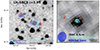 |
Fig. 7. A radio-luminous core in LH-SBC3. Left: IRAC2 image of the LH-SBC3 core area overlaid by the contours of NOEMA 3 mm continuum (blue), LOFAR 150 MHz (cyan) and SPIRE 500 μm (brown dashed). The four confirmed members are marked as red circles and labelled with their IDs. The 3 mm contours start at 2σ in steps of 1σ. The thick cyan contours show the 150 MHz continuum at 6″ starting at 3σ in steps of 1σ. The 500 μm contours are at 20, 40, 60 mJy beam−1 levels. Beams of the 3 mm map, the LOFAR 150MHz at 0.3″ and the LOFAR 150 MHz map at 6″ are shown in the bottom left corner in blue, cyan, and hatched cyan patterns, respectively. Right: zoom-in on the radio galaxy LH-SBC3.a. The cyan contours represent the 150 MHz continuum at 0.3″ starting at 3σ in steps of 1σ. Note that LH-SBC3.d. shows marginal detection of ∼3σ, which reinforces that it is a separate galaxy from LH-SBC3.a. |
Powerful radio AGNs are also revealed in DRC and SPT2349-56 (Oteo et al. 2018; Chapman et al. 2023). Among them, DRC-6 has a radio luminosity similar to LH-SBC3.a, but it is not at the center of the structure. The radio source found in SPT2349-56 is extremely bright, L1.4 GHz, rest = (2.4 ± 0.3)×1026 W Hz−1, 8× brighter than LH-SBC3.a, but this could result from blending several galaxies in the large beams of ATCA and ASKAP. Moreover, in these two cases, the radio galaxies are the main sequence galaxies, unlike the massive and starbursting LH-SBC3.a. Radio-loud galaxies have been used to trace high-z structures. Compared to the radio loud tracers in the CARLA survey (Wylezalek et al. 2013), we find the rest-frame 500 MHz radio luminosity of LH-SBC3.a is at least 1.7 dex lower. Therefore, the starbursting radio core in LH-SBC3 may indicate an early stage of the radio-loud phase when the negative feedback, such as heating from the AGN has not yet come into effect, or it may not evolve to a more powerful stage to impact the host galaxy or the environment negatively. High-redshift radio galaxies (HzRGs) are found to be the most massive galaxies and probable progenitors of BCGs in galaxy clusters (see Miley & De Breuck 2008 for a review). LH-SBC3, together with DRC and SPT2349-56, provides evidence of radio galaxies with vigorous star formation in proto-cluster cores, and the NICE survey will facilitate statistical studies on the probable evolution of radio galaxies into BCGs.
4. Summary
In this paper, we introduce the Noema formIng Cluster survEy (NICE) survey, a 159-h NOEMA large program to search for starbursting massive galaxy groups and clusters at z > 2. We selected candidates by associating SPIRE color-selected IR luminous sources with prominent overdensities of IRAC color-selected massive high-redshift galaxies. This survey will provide us with a statistically large sample to better understand the formation of these structures as well as their influence on the formation and evolution of the galaxies therein.
We verified the feasibility of the NICE candidate selection method by reporting the discovery of a galaxy group at zspec = 3.95, LH-SBC3 from the first quarter of the survey observations. It is spectroscopically confirmed by four galaxies with CO(4-3) and [CI](1–0) line detections within 20″ × 20″ (Fig. 3). All these galaxies are gas-rich and three of them are massive, M⋆ > 1010.5 M⊙. The most massive one, LH-SBC3.a, is a prominent starburst and resides at the centre of the structure. It also hosts a radio AGN with L1.4 GHz, rest = 3.0 × 1025 W Hz−1. The integrated SFR of LH-SBC3 reaches > 4000 M⊙ yr−1, with all the CO-detected members being star-forming and two of them lying significantly above the star-forming main sequence. We estimated the halo mass to be ∼1013 M⊙ and derived a halo mass-normalized total SFR of ∼ 2–10 × 10−10 yr−1, which is around 2 dex higher than the clusters at z = 1–2.
This suggests that the specific SFR per halo mass of clusters continues to grow back in cosmic time, up to z ∼ 4. Together with a few previously discovered similar structures at z ∼ 4, this finding indicates that these compact groups or starbursting cluster cores represent an important phase of massive galaxy assembly in cluster formation.
Acknowledgments
We thank the anonymous referee for the valuable comments. This work is supported by the National Natural Science Foundation of China (NSFC grants 13001103, 12173017 and 12141301). L.Z. and Y.S. acknowledge the support from the National Key R&D Program of China No. 2022YFF0503401, and the National Natural Science Foundation of China (NSFC grants 12121003, 11825302). T.W. acknowledges the support from the China Manned Space Project with No. CMS-CSST-2021-A07. G.E.M. acknowledges the Villum Fonden research grant 13160 “Gas to stars, stars to dust: tracing star formation across cosmic time,” grant 37440, “The Hidden Cosmos,” and the Cosmic Dawn Center of Excellence funded by the Danish National Research Foundation under the grant No. 140. C.G.G. acknowledges support from CNES. Z.J. acknowledges funding from JWST/NIRCam contract to the University of Arizona NAS5-02015. I.D. acknowledges support from INAF Minigrant “Harnessing the power of VLBA towards a census of AGN and star formation at high redshift”. C.d.E. acknowledges funding from the MCIN/AEI (Spain) and the “NextGenerationEU”/PRTR (European Union) through the Juan de la Cierva-Formación program (FJC2021-047307-I). S.J. is supported by the European Union’s Horizon Europe research and innovation program under the Marie Skłodowska-Curie grant agreement No. 101060888. This research used APLpy, an open-source plotting package for Python (Robitaille & Bressert 2012; Robitaille 2019). This work is based on observations carried out under project number M21AA with the IRAM NOEMA Interferometer. IRAM is supported by INSU/CNRS (France), MPG (Germany) and IGN (Spain). This research uses data obtained through the Telescope Access Program (TAP), which is funded by the National Astronomical Observatories, Chinese Academy of Sciences, and the Special Fund for Astronomy from the Ministry of Finance. This work is based on observations obtained with WIRCam, a joint project of CFHT, Taiwan, Korea, Canada, France, at the Canada-France-Hawaii Telescope (CFHT) which is operated by the National Research Council (NRC) of Canada, the Institute National des Sciences de l’Univers of the Centre National de la Recherche Scientifique of France, and the University of Hawaii.
References
- Alberts, S., & Noble, A. 2022, Universe, 8, 554 [Google Scholar]
- Alberts, S., Pope, A., Brodwin, M., et al. 2014, MNRAS, 437, 437 [NASA ADS] [CrossRef] [Google Scholar]
- Alberts, S., Pope, A., Brodwin, M., et al. 2016, ApJ, 825, 72 [NASA ADS] [CrossRef] [Google Scholar]
- Allen, S. W., Evrard, A. E., & Mantz, A. B. 2011, ARA&A, 49, 409 [Google Scholar]
- Behroozi, P. S., Wechsler, R. H., & Conroy, C. 2013, ApJ, 770, 57 [NASA ADS] [CrossRef] [Google Scholar]
- Boquien, M., Burgarella, D., Roehlly, Y., et al. 2019, A&A, 622, A103 [NASA ADS] [CrossRef] [EDP Sciences] [Google Scholar]
- Cai, Z., Fan, X., Bian, F., et al. 2017, ApJ, 839, 131 [NASA ADS] [CrossRef] [Google Scholar]
- Calzetti, D., Armus, L., Bohlin, R. C., et al. 2000, ApJ, 533, 682 [NASA ADS] [CrossRef] [Google Scholar]
- Capak, P. L., Riechers, D., Scoville, N. Z., et al. 2011, Nature, 470, 233 [Google Scholar]
- Carnall, A. C., McLure, R. J., Dunlop, J. S., & Davé, R. 2018, MNRAS, 480, 4379 [Google Scholar]
- Casey, C. M. 2016, ApJ, 824, 36 [CrossRef] [Google Scholar]
- Chabrier, G. 2003, ApJ, 586, L133 [NASA ADS] [CrossRef] [Google Scholar]
- Chapman, S. C., Hill, R., Aravena, M., et al. 2023, ApJ, submitted [arXiv:2301.01375] [Google Scholar]
- Chen, J., Ivison, R. J., Zwaan, M. A., et al. 2023, A&A, 675, L10 [NASA ADS] [CrossRef] [EDP Sciences] [Google Scholar]
- Chiang, Y.-K., Overzier, R., & Gebhardt, K. 2013, ApJ, 779, 127 [Google Scholar]
- Chiang, Y.-K., Overzier, R. A., Gebhardt, K., & Henriques, B. 2017, ApJ, 844, L23 [Google Scholar]
- Coogan, R. T., Sargent, M. T., Daddi, E., et al. 2019, MNRAS, 485, 2092 [NASA ADS] [CrossRef] [Google Scholar]
- Cooke, E. A., Hatch, N. A., Rettura, A., et al. 2015, MNRAS, 452, 2318 [NASA ADS] [CrossRef] [Google Scholar]
- da Cunha, E., Walter, F., Smail, I. R., et al. 2015, ApJ, 806, 110 [Google Scholar]
- Daddi, E., Dannerbauer, H., Stern, D., et al. 2009, ApJ, 694, 1517 [Google Scholar]
- Daddi, E., Valentino, F., Rich, R. M., et al. 2021, A&A, 649, A78 [NASA ADS] [CrossRef] [EDP Sciences] [Google Scholar]
- Dekel, A., Birnboim, Y., Engel, G., et al. 2009, Nature, 457, 451 [Google Scholar]
- Delhaize, J., Smolčić, V., Delvecchio, I., et al. 2017, A&A, 602, A4 [NASA ADS] [CrossRef] [EDP Sciences] [Google Scholar]
- Delvecchio, I., Daddi, E., Sargent, M. T., et al. 2021, A&A, 647, A123 [NASA ADS] [CrossRef] [EDP Sciences] [Google Scholar]
- Galametz, A., Stern, D., De Breuck, C., et al. 2012, ApJ, 749, 169 [NASA ADS] [CrossRef] [Google Scholar]
- Hill, R., Chapman, S., Phadke, K. A., et al. 2022, MNRAS, 512, 4352 [NASA ADS] [CrossRef] [Google Scholar]
- Jin, S., Daddi, E., Liu, D., et al. 2018, ApJ, 864, 56 [Google Scholar]
- Jin, S., Daddi, E., Magdis, G. E., et al. 2019, ApJ, 887, 144 [Google Scholar]
- John, T. L. 1988, A&A, 193, 189 [NASA ADS] [Google Scholar]
- Kereš, D., Katz, N., Weinberg, D. H., & Davé, R. 2005, MNRAS, 363, 2 [Google Scholar]
- Koyama, Y., Smail, I., Kurk, J., et al. 2013, MNRAS, 434, 423 [CrossRef] [Google Scholar]
- Kravtsov, A. V., & Borgani, S. 2012, ARA&A, 50, 353 [Google Scholar]
- Kurk, J. D., Röttgering, H. J. A., Pentericci, L., et al. 2000, A&A, 358, L1 [NASA ADS] [Google Scholar]
- Lemaux, B. C., Le Fèvre, O., Cucciati, O., et al. 2018, A&A, 615, A77 [NASA ADS] [CrossRef] [EDP Sciences] [Google Scholar]
- Liu, D., Gao, Y., Isaak, K., et al. 2015, ApJ, 810, L14 [NASA ADS] [CrossRef] [Google Scholar]
- Liu, D., Daddi, E., Dickinson, M., et al. 2018, ApJ, 853, 172 [Google Scholar]
- Long, A. S., Cooray, A., Ma, J., et al. 2020, ApJ, 898, 133 [NASA ADS] [CrossRef] [Google Scholar]
- Madau, P., & Dickinson, M. 2014, ARA&A, 52, 415 [Google Scholar]
- Magdis, G. E., Daddi, E., Béthermin, M., et al. 2012, ApJ, 760, 6 [NASA ADS] [CrossRef] [Google Scholar]
- Miley, G., & De Breuck, C. 2008, A&A Rev., 15, 67 [NASA ADS] [CrossRef] [Google Scholar]
- Miley, G. K., Overzier, R. A., Zirm, A. W., et al. 2006, ApJ, 650, L29 [NASA ADS] [CrossRef] [Google Scholar]
- Miller, T. B., Chapman, S. C., Aravena, M., et al. 2018, Nature, 556, 469 [CrossRef] [Google Scholar]
- Muldrew, S. I., Hatch, N. A., & Cooke, E. A. 2015, MNRAS, 452, 2528 [NASA ADS] [CrossRef] [Google Scholar]
- Muzzin, A., Wilson, G., Demarco, R., et al. 2013, ApJ, 767, 39 [NASA ADS] [CrossRef] [Google Scholar]
- Oke, J. B., & Gunn, J. E. 1983, ApJ, 266, 713 [NASA ADS] [CrossRef] [Google Scholar]
- Oteo, I., Ivison, R. J., Dunne, L., et al. 2018, ApJ, 856, 72 [Google Scholar]
- Overzier, R. A. 2016, A&A Rev., 24, 14 [NASA ADS] [CrossRef] [Google Scholar]
- Owen, F. N., Morrison, G. E., Klimek, M. D., & Greisen, E. W. 2009, AJ, 137, 4846 [Google Scholar]
- Papovich, C. 2008, ApJ, 676, 206 [NASA ADS] [CrossRef] [Google Scholar]
- Pentericci, L., Kurk, J. D., Röttgering, H. J. A., et al. 2000, A&A, 361, L25 [NASA ADS] [Google Scholar]
- Popesso, P., Biviano, A., Finoguenov, A., et al. 2015, A&A, 579, A132 [NASA ADS] [CrossRef] [EDP Sciences] [Google Scholar]
- Robitaille, T. 2019, Astrophysics Source Code Library [record ascl:1208.017] [Google Scholar]
- Robitaille, T., & Bressert, E. 2012, Astrophysics Source Code Library [record ascl:1208.017] [Google Scholar]
- Salpeter, E. E. 1955, ApJ, 121, 161 [Google Scholar]
- Schreiber, C., Pannella, M., Elbaz, D., et al. 2015, A&A, 575, A74 [NASA ADS] [CrossRef] [EDP Sciences] [Google Scholar]
- Shen, L., Lemaux, B. C., Lubin, L. M., et al. 2021, ApJ, 912, 60 [NASA ADS] [CrossRef] [Google Scholar]
- Steidel, C. C., Adelberger, K. L., Shapley, A. E., et al. 2005, ApJ, 626, 44 [NASA ADS] [CrossRef] [Google Scholar]
- Sweijen, F., van Weeren, R. J., Röttgering, H. J. A., et al. 2022, Nat. Astron., 6, 350 [NASA ADS] [CrossRef] [Google Scholar]
- Tasse, C., Shimwell, T., Hardcastle, M. J., et al. 2021, A&A, 648, A1 [EDP Sciences] [Google Scholar]
- Toshikawa, J., Uchiyama, H., Kashikawa, N., et al. 2018, PASJ, 70, S12 [NASA ADS] [CrossRef] [Google Scholar]
- van der Burg, R. F. J., Muzzin, A., Hoekstra, H., et al. 2014, A&A, 561, A79 [NASA ADS] [CrossRef] [EDP Sciences] [Google Scholar]
- Walter, F., Decarli, R., Carilli, C., et al. 2012, ApJ, 752, 93 [CrossRef] [Google Scholar]
- Wang, T., Elbaz, D., Daddi, E., et al. 2016a, ApJ, 816, 84 [CrossRef] [Google Scholar]
- Wang, T., Elbaz, D., Daddi, E., et al. 2016b, ApJ, 828, 56 [NASA ADS] [CrossRef] [Google Scholar]
- Weaver, J. R., Kauffmann, O. B., Ilbert, O., et al. 2022, ApJS, 258, 11 [NASA ADS] [CrossRef] [Google Scholar]
- Witstok, J., Smit, R., Maiolino, R., et al. 2022, MNRAS, 515, 1751 [Google Scholar]
- Wylezalek, D., Galametz, A., Stern, D., et al. 2013, ApJ, 769, 79 [NASA ADS] [CrossRef] [Google Scholar]
- Zhou, L., Elbaz, D., Franco, M., et al. 2020, A&A, 642, A155 [NASA ADS] [CrossRef] [EDP Sciences] [Google Scholar]
Appendix A: Supplementary data
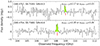 |
Fig. A.1. Spectra of the two galaxies detected at 108GHz as discussed in Section 3. The emission lines are highlighted in yellow with the red vertical bars indicating the line centres. The coordinates, the signal-to-noise ratio of the lines, and the implied redshifts are marked. |
All Tables
All Figures
|
Fig. 1. NICE candidates selection criteria. Left: IRAC color to constrain the redshift to be 2 ≲ z ≲ 4. Data points are UVJ color selected massive SFGs from COSMOS2020 (Weaver et al. 2022). Solid and dashed red curves show the median and the lower limit of 90% of the galaxies. The yellow shade shows the selection criterion. Middle: IRAC2 magnitude to choose galaxies more massive than 1010 M⊙. Data points are UVJ color selected SFGs at 2 < zphot < 4 from COSMOS2020. The red curves and the yellow shade are the same as in the left panel. Right: Herschel/SPIRE colors to select starbursting structures at 2 ≲ z ≲ 4. Grey dots are the Herschel detections in all the NICE survey fields, while the black dots meet the selection criteria in Eq. (2). The blue, red, and magenta curves show the trend of main sequence galaxies, starbursts and SMGs and the circles are marked by the redshifts accordingly. The starbursting proto-cluster at z = 2.51, CL-J1001, is presented as an orange star. See details in Sect. 2.2.2. The inserted histogram displays the distribution of 500 μm fluxes. |
| In the text | |
|
Fig. 2. LH-SBC3 selected following the method in Sect. 2.2. Left: smoothed Σ10 map of the red IRAC priors (Eq. (1)) over the 25′×25′ area around LH-SBC3. The construction of the map is described in Sect. 2.2.1. The inserted histogram is the distribution of Σ10 (black histogram) and the Gaussian fit (red dashed curve). The red arrow indicates the peak Σ10 value of LH-SBC3. Right: Herschel/SPIRE composite color image of the same area. The R, G, and B channels correspond to 500 μm, 350 μm, and 250 μm, respectively. The white circles in both figures have a radius of 2′. |
| In the text | |
|
Fig. 3. The four members of LH-SBC3 spectroscopically confirmed by NOEMA. Left: NOEMA spectra of four confirmed cluster members. The channel width of the spectra is rebinned to be ∼150 km s−1. The detected lines are highlighted in yellow. CO(4–3) and [CI](1–0) frequencies are marked by vertical bars in red and blue, respectively. Right: 3 mm continuum images of the four members overlaid by CO(4–3) intensity contours in yellow. The red circles denote the positions of the galaxies determined by the flux peak of the 3 mm continuum. The CO(4–3) intensity contours start at 1σ (equivalent to ∼56 mJy km−1 beam−1) in steps of 1σ. Beams of the 3 mm and CO(4–3) intensity maps are shown in the second panel as black-hatched and yellow patterns corresponding to 3.43″ × 3.60″and 2.37″ × 2.02″, respectively. |
| In the text | |
|
Fig. 4. Left: spatial distribution of galaxies with photometric redshift intervals consistent with z = 3.95. The dashed box denotes the 1′ × 1′(∼2 cMpc × 2 cMpc) region of the galaxy overdensity, LH-SBC3. The dots are color-coded by their stellar masses. Right: zoom-in RGB image (red: IRAC2; green: K; blue: i) of LH-SBC3. The white solid contours denote the 3 mm continuum, starting at 2σ in steps of 1σ. The four CO-confirmed members are labelled with their IDs. Note: LH-SBC3.a and d are very close. The cyan dashed circles are the IRAC-color selected priors. The priors labelled with a question mark could come from another structure at z = 3.25 or z = 2.19, see discussion in Sect. 3. The dotted white contours show 500 μm flux at 20, 40, 60 mJy beam−1 levels. |
| In the text | |
|
Fig. 5. FIR SED of LH-SBC3. Line-of-sight contamination to the SPIRE fluxes is subtracted using the deblending procedures in Jin et al. (2018). The 3 mm flux is well fitted by an optically thin dust model (Witstok et al. 2022). |
| In the text | |
|
Fig. 6. Position of the LH-SBC3 member galaxies (red circles) with respect to the star-forming main sequence at z = 4 (Schreiber et al. 2015). Galaxies in the Dense Red Core (DRC, z = 4; Oteo et al. 2018; Long et al. 2020) and SPT2349-56 (z = 4.3, Miller et al. 2018; Hill et al. 2022) are shown as magenta and green circles, respectively. |
| In the text | |
|
Fig. 7. A radio-luminous core in LH-SBC3. Left: IRAC2 image of the LH-SBC3 core area overlaid by the contours of NOEMA 3 mm continuum (blue), LOFAR 150 MHz (cyan) and SPIRE 500 μm (brown dashed). The four confirmed members are marked as red circles and labelled with their IDs. The 3 mm contours start at 2σ in steps of 1σ. The thick cyan contours show the 150 MHz continuum at 6″ starting at 3σ in steps of 1σ. The 500 μm contours are at 20, 40, 60 mJy beam−1 levels. Beams of the 3 mm map, the LOFAR 150MHz at 0.3″ and the LOFAR 150 MHz map at 6″ are shown in the bottom left corner in blue, cyan, and hatched cyan patterns, respectively. Right: zoom-in on the radio galaxy LH-SBC3.a. The cyan contours represent the 150 MHz continuum at 0.3″ starting at 3σ in steps of 1σ. Note that LH-SBC3.d. shows marginal detection of ∼3σ, which reinforces that it is a separate galaxy from LH-SBC3.a. |
| In the text | |
|
Fig. A.1. Spectra of the two galaxies detected at 108GHz as discussed in Section 3. The emission lines are highlighted in yellow with the red vertical bars indicating the line centres. The coordinates, the signal-to-noise ratio of the lines, and the implied redshifts are marked. |
| In the text | |
Current usage metrics show cumulative count of Article Views (full-text article views including HTML views, PDF and ePub downloads, according to the available data) and Abstracts Views on Vision4Press platform.
Data correspond to usage on the plateform after 2015. The current usage metrics is available 48-96 hours after online publication and is updated daily on week days.
Initial download of the metrics may take a while.