| Issue |
A&A
Volume 685, May 2024
|
|
|---|---|---|
| Article Number | A142 | |
| Number of page(s) | 17 | |
| Section | Astrophysical processes | |
| DOI | https://doi.org/10.1051/0004-6361/202348230 | |
| Published online | 17 May 2024 | |
Fitting the light curves of Sagittarius A* with a hot-spot model
Bayesian modeling of QU loops in the millimeter band
1
Department of Astrophysics/IMAPP, Radboud University, PO Box 9010 6500 GL Nijmegen, The Netherlands
e-mail: a.yfantis@astro.ru.nl
2
Max-Planck-Institut für Radioastronomie, Auf dem Hügel 69, 53121 Bonn, Germany
3
Research Centre for Computational Physics and Data Processing, Institute of Physics, Silesian University in Opava, Bezručovo nám. 13, 746 01 Opava, Czech Republic
Received:
11
October
2023
Accepted:
17
February
2024
Context. Sagittarius A* (Sgr A*) exhibits frequent flaring activity across the electromagnetic spectrum. Signatures of an orbiting hot spot have been identified in the polarized millimeter wavelength light curves observed with ALMA in 2017 immediately after an X-ray flare. The nature of these hot spots remains uncertain.
Aims. We expanded existing theoretical hot-spot models created to describe the Sgr A* polarized emission at millimeter wavelengths. We sampled the posterior space, identifying best-fitting parameters and characterizing uncertainties.
Methods. Using the numerical radiative transfer code ipole, we defined a semi-analytical model describing a ball of plasma orbiting Sgr A*, threaded with a magnetic field and emitting synchrotron radiation. We then explored the posterior space in the Bayesian framework of dynesty. We fit the static background emission separately, using a radiatively inefficient accretion flow model.
Results. We considered eight models with a varying level of complexity, distinguished by choices regarding dynamically important cooling, non-Keplerian motion, and magnetic field polarity. All models converge to realizations that fit the data, but one model without cooling, non-Keplerian motion, and magnetic field pointing toward us improved the fit significantly and also matched the observed circular polarization.
Conclusions. Our models represent observational data well and allow testing various effects in a systematic manner. From our analysis, we have inferred an inclination of ∼155 − 160 deg, which corroborates previous estimates, a preferred period of ∼90 min, and an orbital radius of 9 − 12.0 gravitational radii. Our non-Keplerian models indicate a preference for an orbital velocity of 0.6–0.9 times the Keplerian value. Last, all our models agree on a high dimensionless spin value (a* > 0.8), but the impact of spin on the corresponding light curves is subdominant with respect to other parameters.
Key words: black hole physics / magnetic fields / polarization / methods: numerical / methods: statistical / Galaxy: center
© The Authors 2024
 Open Access article, published by EDP Sciences, under the terms of the Creative Commons Attribution License (https://creativecommons.org/licenses/by/4.0), which permits unrestricted use, distribution, and reproduction in any medium, provided the original work is properly cited.
This article is published in open access under the Subscribe to Open model. Subscribe to A&A to support open access publication.
1. Introduction
The supermassive black hole (SMBH) at the center of our Galaxy, Sagittarius A*, is surrounded by a hot accretion flow comprising relativistic plasma that emits bright synchrotron radiation. Several decades of radio as well as infrared, X-ray, and γ-ray observations of Sgr A* led to a detailed model for the accreting structure in the close vicinity of this SMBH (e.g., Narayan et al. 1995; Quataert & Gruzinov 2000; Yuan et al. 2003). The strongly sub-Eddington luminosity of Sgr A* (LBol ∼ 10−8 LEdd) and high rotation measure (RM) toward the source indicate that the accretion rate is Ṁ ≈ 10−9−10−7 M⊙ yr−1 (e.g., Marrone et al. 2006; Event Horizon Telescope Collaboration 2022a). This low accretion rate for a 4 × 10⁶ M⊙ SMBH is only feasible via an advection-dominated accretion flow (ADAF) mode, and the observed emission is either the ADAF itself (Narayan et al. 1998), a jet launched by the ADAF (Falcke & Markoff 2000), or both (Yuan et al. 2002). Until recently, the main difficulty in elucidating the nature of the Sgr A* emission was the scattering screen that smears the radio view of the source up to millimeter waves (Issaoun et al. 2019, and references therein).
Recent observations of Sgr A* at millimeter wavelengths (λ = 1.3 mm, ν = 230 GHz) by the Event Horizon Telescope (EHT) for the first time revealed detailed images of the event-horizon-scale emission in the Galactic center (Event Horizon Telescope Collaboration 2022b, 2022c). The EHT observations are broadly consistent with predictions of the ADAF model realized via general relativistic magenetohydrodynamic (GRMHD) simulations (Event Horizon Telescope Collaboration 2022a). However, when comparing a large library of GRMHD simulations (with different black hole spins and multiple ion-electron temperature ratios, magnetic field strengths, and geometries) it has been found that one of the most prominent differences between numerical models of ADAF and millimeter observations of Sgr A* is the variability; the models are too variable in amplitude by a factor of two compared to the light-curve data (Event Horizon Telescope Collaboration 2022a; Wielgus et al. 2022a). This discrepancy between observations and models can be associated with two main uncertainties in the models. The first uncertainty is the unknown global geometry and stability of magnetic fields in ADAFs. The second even more problematic uncertainty is the poorly understood thermodynamics and acceleration of radiating electrons in a collisionless plasma, which is characteristic of ADAF solutions. These two main uncertainties prevent us from determining the spin of Sgr A* and understanding whether the observed photons originate in the accretion disk or at the jet base. Moreover, the challenges to explain all Sgr A* observational constraints using a single simulation are expected to increase rapidly as more detailed observational data sets are obtained. We have therefore entered an era of precision astrophysics, in which quantitative tests of theoretical predictions can be performed with event-horizon-scale astronomical observations.
Building a global model of a collisionless accretion flow and jet for Sgr A* using first-principle approaches, such as general relativistic particle-in-cell (GRPIC) simulations, where the electron thermodynamics and acceleration is calculated self-consistently, is currently impossible. This is mostly due to the computational complexity of the problem. GRPIC models are therefore mostly only focused on modeling outflowing magnetospheric electron-positron emission, often with unrealistic boundary conditions (Crinquand et al. 2022), or on simplified zero-angular momentum accretion models (Galishnikova et al. 2023). Another more computationally feasible approach is to model Sgr A* emission using semi-analytic models (e.g., Broderick & Loeb 2006; Broderick et al. 2011; Younsi & Wu 2015; GRAVITY Collaboration 2018, 2020a,b; Ball et al. 2021; Vos et al. 2022). These are particularly useful because a large parameter survey can be carried out a model like this is fit to observational data.
In this work, we fit the polarized observations of Sgr A* near event-horizon emission reported by Wielgus et al. (2022b; hereafter W22) with semi-analytic models. Our main goal is to give insight into possible conditions of collisionless plasma around Sgr A*, independent of the GRMHD and GRPIC interpretation. A byproduct of our fitting procedure is the determination of the spin of Sgr A*, its orientation on the sky, and the observer’s viewing angle geometry. These can be compared to geometrical parameters inferred from different types of data such as all EHT images (Event Horizon Telescope Collaboration 2022a,b,c) or results from GRAVITY (e.g., GRAVITY Collaboration 2018, 2020a,b; GRAVITY Collaboration 2023).
We used polarization data from the Atacama Large Millimeter/submillimeter Array (ALMA), which observed Sgr A* in April 2017. We focused on 230 GHz data that were collected immediately following an X-ray flare detected by the Chandra observatory on April 11 2017 (Event Horizon Telescope Collaboration 2022d; Wielgus et al. 2022a). The data set was presented and interpreted in W22, who found that Sgr A* polarimetric ALMA light curves show so-called 𝒬 − 𝒰 loops, which can be well described by a model of a Gaussian hot spot threaded by a vertical magnetic field on an equatorial orbit around a Kerr black hole (Gelles et al. 2021; Vos et al. 2022; Vincent et al. 2024). In previous works, only a very limited range of the spot model parameters (mostly geometrical parameters) have been explored (W22, Vos et al. 2022). In this work, we couple our semi-analytic model of an orbiting spot around the Kerr black hole to a Bayesian parameter estimation framework, which allows us to carry out a large survey of the physical and geometrical parameters. The current work also presents two main extensions to our previous model. We now also simulate in an approximate way the cooling of the hot spot. Observational indications of the dynamical importance of cooling after the X-ray flare were reported in Appendix G of W22. Additionally, we allow the spot to be on a non-Keplerian circular orbit, which was only briefly discussed in Appendix C of W22 and was studied theoretically by Vos et al. (2022). Our results have important implications for the GRMHD and GRPIC simulations, which are built to model Sgr A*, regarding the plasma conditions and dynamics.
The manuscript is structured as follows. In Sect. 2 we briefly describe our semi-analytic model of a hot spot around Sgr A*. In Sect. 3 we outline the data properties, our fitting framework, and the procedure. The results are presented in Sect. 4. We discuss the implications and provide conclusions in Sect. 5.
2. Model
To simulate millimeter emission from the flaring Sgr A*, we adoptede and further developd the semi-analytic model described in full detail by Vos et al. (2022). The model is inspired by work of Broderick & Loeb (2006; see also Fraga-Encinas et al. 2016). It consists of a semi-analytic model of a stationary accretion flow and a time-dependent component of an orbiting bright spot around a Kerr black hole. The model is fully built within ipole, which is a ray-tracing code for the covariant general relativistic transport of polarized light in curved space-times developed by Mościbrodzka & Gammie (2018). The ipole code was used, among other applications, to generate the EHT library of template black hole images based on GRMHD simulations (e.g., Event Horizon Telescope Collaboration 2022a).
To calculate thermal synchrotron emission (we assumed that electrons have a relativistic thermal energy distribution function; see Vincent et al. 2024, for a different approach), the radiative transfer model necessitates the specification of the underlying density, electron temperature, and magnetic field characteristics of the plasma. After the plasma configuration is defined, ipole generates maps of Stokes 𝓘,𝒬,𝒰, and 𝒱 at the selected observing frequencies. The underlying calculations employ the full relativistic radiative transfer model of ipole, including synchrotron emission, self-absorption, and the effects of Faraday rotation and conversion. Because Sgr A* indicates a moderate Faraday depth at 230 GHz, with a Faraday screen most likely collocated with the compact emission region (Wielgus et al. 2024), it may be necessary to incorporate a complete radiative transfer into the model for a quantitative comparisons with observations. We self-consistently accounted for the finite velocity of light, that is, we did not employ the commonly used fast light approximation.
The model is divided into two components: a static background, modeling a radiatively inefficient ADAF disk, and an orbiting hot spot. For the background variables, we used the bg subscript, and the governing equations read
where ne is the electron number density, σ = 0.3 characterizes the disk vertical thickness, Θe = kbTe/mec2 is the dimensionless electron temperature, Bbg is the magnetic field strength, rg = GM/c2 is the gravitational radius, r, θ are the coordinates, and n0, bg, Θ0, bg, B0, bg are the values at the center (r = 0). The field has a vertical orientation, unless specified otherwise (poloidal, or radial possibilities), with one of two possible polarities. The background ADAF is either on a fixed Keplerian orbit or deviates from it according to the parameter Kcoef, which corresponds to a period P of
where Kcoef is a parameter controlling the Keplerianity of the orbit (for Kcoef = 1, the disk orbit is Keplerian, and for Kcoef < 1, it is sub-Keplerian). In our model, all emission is cut below the innermost stable circular orbit (ISCO). The space-time is described with the Kerr metric, with the standard metric signature (− + + +) and dimensionless black hole spin a* = Jc/GM2. The units are natural (c = G = 1), hence, distance and time can be conveniently measured in units of M (M ≡ rg ≡ rg/c). We assumed a mass of Sgr A* M = 4.155 × 10⁶ M⊙, which is between the measurements of GRAVITY Collaboration (2022) and those of Do et al. (2019).
The second component of the model is the spot. The spot lies in a circular orbit in the equatorial plane, and its location in Kerr–Schild coordinates is defined as
Here, t is the coordinate time (in units of M), rs is the radial distance from the black hole center (also in units of M), and P is the orbital period defined in Eq. (2).
The plasma density, temperature, and magnetic field strength in the spot are then described by
where n0, s, Θ0, s, and B0, s are the values at the center of the spot, Δx is the Euclidean distance from the spot center to the photon emission site, connected to the distant observer’s screen with a null geodesic. Rs is the size of the Gaussian standard deviation, defining the size of the spot, and it remained fixed at 3 M to limit the number of parameters. Additionally, we used a spot boundary, ignoring matter when ne, s ≤ 0.01n0, s to limit the Gaussian “tail”.
We extended the spot models of Vos et al. (2022) and allowed the Gaussian spot to change its temperature as an exponential function of time. This is a simplistic general prescription that does not aim to simulate the synchrotron cooling, but rather enabled us to explore the impact of cooling without making additional assumptions regarding its physical mechanisms. We introduce the cooling coefficient Ccoef and the numerical parameter Tini = 2000 M, which guarantees that the spot cooled when Ccoef > 0 (we note that ipole tracks light backward in time from the camera position at r = 1000 M so that the coordinate time t is a negative quantity). The spot does not cool when Ccoef = 0.
Two numerical parameters of our model remain: the image field of view (FOV), and its resolution. We adopted FOV = 40 M ≈ 200 μ as because most of the millimeter emission of Sgr A* is generated close to the black hole event horizon, with the black hole shadow ring diameter observed by the EHT corresponding to around 10–11 M (Event Horizon Telescope Collaboration 2022b,e). Synthetic light curves were then generated by creating snapshot images at a predefined sequence of times and integrating their intensities over the FOV into total flux densities in all four Stokes parameters. Due to large numerical cost of these calculations, we adopted a resolution of 64 × 64 pixels per single frame. An analysis of the effects of the image resolution on the simulated light curves can be found in Appendix A, where we justify the intermediate value of the resolution we chose. Our reasoning was that despite some fractional differences in parts of the curves, the general behavior remains very similar and the relative differences are below the error level of the data.
3. Two-step parameter estimation procedure
ALMA observed Sgr A* on April 11, 2017, from 9 UTC until 13 UTC. Stokes 𝒬 − 𝒰 loops, interpreted as a signature of a bright spot around the black hole, were observed within the first two hours of this observing window. We fit ALMA light curves starting at 9:00 UTC until 10:30 UTC (see Fig. 1). Hence, the data segment we considered begins 20 min earlier than the segment used by W22. Our original data set had 710 data points, but we used 35 of these, sampling 1 out of 20 points. Within this time, the ALMA data have a few gaps in which it observed Sgr A* calibrators. In our modeling, we only fit Stokes 𝒬 and 𝒰 light curves, but we verified Stokes ℐ and 𝒱 for consistency afterward because we assumed that during the 𝒬 − 𝒰 loop, the strongest signal of the spot is visible in the linear polarization rather than in total intensity and circular polarization, which may be dominated by the black hole shadow component originating close to the event horizon of the black hole and associated with the background image of the accretion flow (W22).
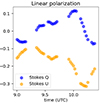 |
Fig. 1. Observed Sgr A* light curves for Stokes 𝒬 and 𝒰 from ALMA (W22). We only plot the points of the 35 time stamps that were used to infer the model parameters and not the 710 time stamps from the original light curve. |
To model the ALMA data, we set up a fitting framework that combined our ipole simulations with the dynesty software, introduced by Speagle (2020) and further developed by Koposov et al. (2023). dynesty is a Bayesian tool capable of performing dynamic nested sampling. It was introduced for computational usage in Skilling (2006). Given our model light curves, dynesty proved to be an excellent choice for our framework because it is compatible with low-dimensional but highly degenerate and potentially multimodal posteriors (e.g., Palumbo et al. 2022). We embedded ipole so that the sampler called a ray-tracing operation for every log-likelihood evaluation.
The posterior landscape of our model is very complex, and our model for the background emission (the shadow component) neither includes emission from regions within the ISCO nor has any variability. We therefore decided to simplify our fitting procedure. We introduced a two-step fitting scheme in which the spot light curve was fit separately from static background emission as follows. In our first fitting step, we fit emission from the spot alone, and in this step, the background linear polarization was modeled as the 𝒬sha and 𝒰sha parameters (where sha stands for shadow, following W22), which were simply added to the variable light curves. In our second fitting step, we fit the static background model to the estimated pair of (𝒬sha, 𝒰sha), which represents an average emission from near the shadow of the black hole that is always visible in the millimeter waves. This split in the fitting procedure works well as long as both Faraday effects between components are negligible, for example, when the two model components are spatially separated in the images. As shown below, our spot is usually located at r > 10 M with very narrow posterior distributions, so that the spot and the near horizon emission are usually well separated.
To be able to produce a fit on timescales shorter than a year, we sub-sampled the ALMA data set of W22 by a factor of 20, which changed cadence very little from 4 s to 80 s. Hence, we fit only 35 data points (or rather 70 because we took 𝒬 and 𝒰 values into account separately). Because of the temporal correlation timescales involved, the subsampling has little impact on the inference power. We finally had with a scheme that performed a single log-likelihood evaluation in less than 3 s, using 24 cores1.
The time per log-likelihood calculation requires a configuration for dynesty that converges with the least number of iterations. To do this, we used a dynamic sampler that was introduced by Higson et al. (2019) with 200 initial live points and 200 points per extra dynamical batch (10 in total). We used the default stopping criteria, meaning a terminating change in the log-evidence of 0.01. Additionally, we adopted a weight function that shifted the importance of the posterior exploration (rather than the evidence) to 100%. Last, we used “overlapping balls” that can generate more flexible bounding distributions. The balls were first mentioned in Buchner (2016). We also used a random walk as our sampling technique. This was developed by Skilling (2006).
Our log-likelihood function is defined in a standard way as
![$$ \begin{aligned} \mathcal{L} (\boldsymbol{p})=-\sum _j\frac{\left[Q_j-\hat{Q}_j(\boldsymbol{p})\right]^2}{2\sigma _{Q,j}^2} + \frac{\left[U_j-\hat{U}_j(\boldsymbol{p})\right]^2}{2\sigma _{U,j}^2}, \end{aligned} $$](/articles/aa/full_html/2024/05/aa48230-23/aa48230-23-eq5.gif)
where p is the vector of the parameters that are to be estimated, and Qj , Uj and  are the observed and modeled Stokes 𝒬 and 𝒰 for every data point (j). The modeled quantities were directly calculated during the ray-tracing. The errors are defined as
where ϵs = 0.02 is the assumed systematic error, and ϵt = 0.01 represents thermal noise. For the characterization of uncertainties in the ALMA data see Wielgus et al. (2022a), where the formal ALMA light-curve uncertainties were found to be underestimated. The reduced χ2 then naturally follows as
where χ2 = −2ℒ, nd = 70 , (2 × 35) is the number of data points, and nf = 10, 11, or 12 is the number of degrees of freedom, which is equal to the number of parameters that were fit simultaneously.
A comprehensive list of all the parameters and their ranges used in our fitting pipeline, referred to as bipole in the next sections, is shown in Table 1. For n0, s, Θ0, s, and B0, s we sampled the log space with Gaussian priors centered in the middle of their log ranges (i.e., log-normal priors). For the remaining parameters we considered, we assume flat priors.
Parameters and prior ranges used for the fitting.
Finally, before fitting the real data, we performed a controlled bipole run using synthetic data to demonstrate the ability of our pipeline to recover the truth value. The total number of fitted parameters was the same as for the real data (see Sect. 4) with the same priors. The results are presented in Fig. 2. On the left side, we present the trace plot, showing the evolution of the live points throughout the run. On the right side, we show the corner (or triangle) plot, showing the single and joint distributions for all parameters. All truth values, indicated with red lines, are comfortably covered by the posteriors. Additionally, we observe a correlation between the plasma parameters (n0, s Θ0, s, B0, s) that is expected for synchrotron emission, a correlation between rs and Kcoef, which is expected given the period relation, and an overall less strictly constrained Ccoef posterior, which is expected given the volatility of this parameter for small changes in plasma parameters.
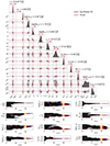 |
Fig. 2. Triangle and trace plots of the synthetic light-curve fitting. Top: Triangle plot, a combination of 1D and 2D marginalized posteriors, with the dashed lines denoting the median and 2σ or (90%) confidence levels (left and right). Similarly, the contours are for 90% (outer) and then 50% and 25% confidence levels. The truth is marked with red lines. Bottom: Trace plots showing the evolution of particles (and their marginal posterior distributions) in 1D projections, where lnX denotes the prior volume of the parameter space. The dots are color-coded with respect to their relative posterior mass, meaning that bright yellow values are present when convergence is achieved. |
4. Results
4.1. Spot fitting
We ran eight models that we list in Table 2 to fit the spot component to the ALMA observational data. The set of models was composed of all combinations of three criteria: (1) no cooling or fitting the cooling parameter Ccoef; (2) prescribed default or flipped magnetic field orientation; in the default models, the magnetic field vector was aligned with the black hole spin, which is also aligned with the angular momentum vector of the hot spot, which points away from us for the prior space of inclination (i > 90°); and (3) assumed Keplerian motion, or fitting a non-Keplerianity parameter Kcoef. The models were labeled to contain the information of the specific case. The first part refers to cooling (nc being no cooling), the second part to Bfield, and the last part to a Keplerian orbit (nk being the non-Keplerian orbit). We report below the posteriors from each run, discuss the goodness of fit, and show the produced light curves with the best parameters from every model.
Models used to fit Sgr A* ALMA data.
In Fig. 3 (top part) we show the posterior distributions for all parameters for two different magnetic field orientations in Keplerian models without cooling (nc_db_k, nc_fb_k). The first important feature to note is the agreement in the value of inclination for both models, which matches the fiducial model of W22, who assumed an inclination of 158 deg. Second, the values of rs are identical in the models (rs = 11.65 M and with narrow posteriors), but larger than those of W22, who assumed 10 − 11 M. This has a direct effect on the loop period (Eq. (2), for rs ∼ 10 M and fixed Keplerian motion spin has little effect), producing a period of T = 88 min, which is longer than the 70 min proposed in W22. This is further discussed in the next Sect. 5. The black hole spin is constrained at the upper end of the prior space (a* ∼ 0.9); this is further discussed in Sect. 5. The plasma density, electron temperature, and magnetic field strengths are normally distributed around n0, s ∼ 107 particles/cm−3, and Θ0, s ∼ 40, B0, s ∼ 5 G. There is also a correlation between n0, s, Θ0, s and B0, s similar to the synthetic data fit. The PA values lie around zero. Between the default and flipped Bfield fits, some parameters exhibit noticeable shifts, among which Qsha is most significantly affected (see Sect. 4.3). From the reported log(Evidence) alone, there is no strong preference for either of the two Bfield orientations. In the bottom part of Fig. 3, we present the light curves and the 𝒬 − 𝒰 loop using the model with the highest likelihood from each run as parameters for the ray-tracing. In the lower left corner of the light curve, we report the lowest  value. The nc_fb_k model has
  , that is, half of the
  for nc_db_k model.
For the second family of models used in the fitting pipeline (c_db_k, c_fb_k), we incorporated an additional parameter, namely Ccoef ≠ 0, which permits the time evolution of the electron temperature values in the spot according to Eq. (4). In Fig. 4 (top panels) we show the posterior distributions for all free parameters of this model. The inclination is consistent between the two orientations of Bfield and with the no-cooling models nc_db_k and nc_fb_k. In the case of c_db_k, the remaining parameters are also very similar to the models without cooling, but the plasma parameters show longer tails. This effect arises because Ccoef spans an order of magnitude with 2σ confidence. In contrast, in the case of c_fb_k, the remaining distributions exhibit many differences. First, there is a prominent bimodal character to the posteriors that affects all parameters except for the plasma parameters. Second, the plasma parameters do not remain similar either, with a modification of the synchrotron emission caused by higher Bfield values ( ∼ 60 G) and lower densities and temperatures (106 and 10, respectively). Of the two realizations of c_fb_k, the realization with high spin seems more likely because it produces a period of T = 91 min, while the other realization produces T = 101 min. The cooling coefficient is the same as the default Bfield (Ccoef ∼ 10−5 − 10−4), producing a drop in temperature ranging from 0.01% to 2% during the simulation (light-curve duration of ∼1.5 h). In the bottom panels of Fig. 4, we present the model c_b and c_fb light curves and the 𝒬 − 𝒰 loop using the highest likelihood models from each run as parameters for the ray-tracing. Their  is reported in the lower left corner of the figure. The two models with cooling again prefer high black hole spins, while
  and
and  here are twice higher than the values reported for model nc_fb_k. Models without and with cooling have similar Evidence.
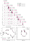 |
Fig. 3. Triangle plot and light curves for the Keplerian spot models without cooling (Kcoef = 1, Ccoef = 0). Top: Triangle plot of the posterior distributions for all parameters. The results for the two magnetic field polarities are shown in different colors, and their respected log(Evidence) values are reported in the label. Bottom: Best-fit model 𝒬 − 𝒰 light curves and 𝒬 − 𝒰 loops (color points) overplotted with ALMA observational data (gray points). The |

In Fig. 5 (top panels) we show the posterior distributions for all free parameters for the non-Keplerian model without cooling (models nc_db_nk and nc_fb_nk with Kcoef ≠ 1, Ccoef = 0). The differences between the two Bfield orientations are enhanced. Model nc_fb_nk produces a strikingly high log(Evidence) = −50 that distinguishes it among all other models, with log(Z) < − 63. The consistency in inclination and spin values persists, but the values for the spot radius are significantly lower (rs = 9 − 10 M). This is a direct effect of non-Keplerian motion expressed as subunit values of Kcoef = 0.6 − 1.0. The light curves are shown in the bottom panels of Fig. 5 together with the  values of each model. The low value of
  together with the log(Evidence) and the smooth posteriors make nc_fb_nk our best-bet model.
In Fig. 6 (top panels) we show the posterior distributions for all free parameters for the non-Keplerian model with cooling (models c_b_nk and c_fb_nk with Kcoef ≠ 1, Ccoef ≠ 0). The inclination and spin are still the same, but the two Bfield orientations again behave very differently when cooling is included. While both cases have a similar Ccoef range, Kcoef behaves much differently than in the nc_db_nk and nc_fb_nk cases. The c_db_nk has a wide Kcoef = 0.8 − 1.2 that correlates well with rs, while c_fb_nk has a narrow Kcoef = 0.5 that in combination with rs = 10.8 M does not reproduce the required period. The log(Evidence) for both models is lower than in any of the remaining models, but in particular, for c_fb_nk the Evidence together with the  make the fit most unreliable. The light curves are shown in the bottom panels of Fig. 6.
The orbital periods of most of the best-fit models (with just one exception) fall into a narrow range between 87 and 93 min, which corresponds to the duration of our fit light curve (1.5 h). For comparison, the model c_fb_nk has a much longer period of approximately 155 min. All orbital periods of the spots are reported in Table 5 in Sect. 5.
4.2. Cross-checking with other Stokes parameters
In this section, we report the behavior of the Stokes ℐ and 𝒱 light curves for the best-fit realizations of the eight discussed models. The goal is to verify the consistency of the models with the remaining observational information that was not used in the fitting procedure because of the model limitations listed in Sect. 3.
In the top row of Fig. 7, we present the Stokes ℐ light curves for all spot models. The shift (sha) of the light curves is just for visual aid, and it accommodates the contribution we expect from the background (the accretion disk). We did not fit for the best “shadow” (sha) values to Stokes ℐ (and 𝒱, see below). We observe only a small variation in Stokes ℐ in all models. This is expected since Stokes ℐ should be largely dominated by the background emission, and any variations could be due to the background variability, which we did not model here.
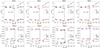 |
Fig. 7. Stokes ℐ, 𝒱 light curves for all models compared to the observational data from Wielgus et al. (2022a) and W22 (obs). The arrows represent a constant background component to facilitate comparison with the real data. |
In the bottom row of Fig. 7, we show the light curves for Stokes 𝒱. All models with flipped Bfield except for one model exhibit a behavior that resembles the data more closely than the default Bfield models. When we apply a shift with the same shadow concept as for Stokes ℐ, the coincidence with the data is evident. In particular, the best-bet model nc_fb_nk recovers the observed Stokes 𝒱 best, which is a strong independent argument in support of the model.
4.3. Background emission
Here, we report the second part of our two-step fitting algorithm. We fit the 𝒬sha, 𝒰sha values from every model (reported in Table 3) with the ADAF model described by Eqs. (1). Our goal was to obtain the density, temperature, and magnetic field strengths of the background component. To fit the plasma parameters of the background emission, we fixed all the geometric parameters (a*, i, PA), plus Kcoef for non-Keplerian models, at the values obtained in the spot-fitting (during the first step). The choice to simulate the disk with the same Kcoef as the spot is an assumption because other possibilities could be meaningful as well, for instance, a Keplerian disk with a sub-Keplerian spot. The exclusion of the radiation originating inside the ISCO constitutes an additional limitation. Last, we note that since the background is static, we only need one point (or rather two, for 𝒬 and 𝒰) to make the fit.
𝒬sha, 𝒰sha values for all models obtained in the first fitting step, as well as the average values of 𝒬 and 𝒰 from the ALMA data.
In Fig. 8 we show the posteriors from the aforementioned background models. All runs converge, but there is a clear difference between the two Bfield orientations, which is the level of correlation. The default Bfield has higher correlations, which is an indication that it might describe the background emission better. The values for all three parameters are roughly higher by an order of magnitude than what we expect, but this is most likely due to the lack of radiation from within the ISCO.
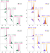 |
Fig. 8. Triangle plots for the background solution. The geometric parameters (i, a, PA), and Kcoef for nk cases were fixed at the values of the initial runs for the two Bfield orientations (color-coded) and without (left panels) and with cooling (right panels). |
Using the peaks of the posteriors from the three parameter runs, we calculated Stokes ℐBG, 𝒱BG produced from the background disk. Our motivation was to test whether any of the Stokes values match the reported ℐsha, 𝒱sha values used in Fig. 7. The values are reported in Table 4. All values from the default Bfield models match the shadow components fairly well. Moreover, the models with a flipped magnetic field orientation produce opposite values for Stokes 𝒱BG. We comment on the implications of these results in Sect. 5. Overall, this second step does not offer much inferring power at this point, but it serves as a pointer for the preferred Bfield orientation and is a sanity check and validation of our overall approach of splitting the fitting into two steps.
5. Discussion and conclusions
We generate a family of semi-analytic models of an accretion flow with a bright orbiting spot to fit Sgr A* millimeter data recorded by ALMA on April 11, 2017. Our models have a varying number of the degrees of freedom. The question which model represents the observational data best can be answered using either Bayesian or physical arguments.
The model that reproduces the data best, that is, corresponds to the lowest  parameter, is shown in Fig. 9, made with a flipped Bfield, no cooling, and a non-Keplerian orbit. Based on the
  , the two best models are with a flipped Bfield (magnetic field vector arrow pointing toward the observer for viewing angles i > 90 deg). It is worth pointing out that the only difference between the two orientations comes from Faraday effects, and particularly, rotation. Additionally, in Table 5, we report all the log-Evidence (marginal likelihood) from all models. Most models produce similar values, with two exceptions: nc_fb_nk, with a significantly higher value, and the two cooling and non-Keplerian models with a lower value.
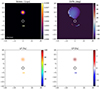 |
Fig. 9. Snapshot from the end of the light curve from our best-fitting model (nc_fb_nk), using 642 resolution, for Stokes ℐ, EVPA, fractional linear polarization (LP), and fractional circular polarization (CP). |

Based on physical arguments, the models that describe the observations best are those that in addition to Stokes 𝒬 and 𝒰 also show some consistency with the observed Stokes 𝒱 (also see Appendix E of W22). The model that satisfies this requirement particularly well is still the one without cooling and no-Keplerian orbits. All models with a default magnetic field orientation fail to recover the Stokes 𝒱 variability. We also find a mismatch between the modeled and observed Stokes ℐ during the flare, but this is expected. Stokes ℐ during the flare could be dominated by the background emission, which may be changing as well. The observed total intensity light curve appears to recover from the minimum following the X-ray flare, steadily increasing the flux density on a timescale of ∼2 h, which may be interpreted as the accretion disk cooling down after the energy injection (Wielgus et al. 2022a). Alternatively, Stokes ℐ during the flare may be also influenced by spot properties that we did not include in our simple model, such as the shearing of the spot or other spot interaction with the background flow (e.g., Tiede et al. 2020).
In observational data, the 𝒬 − 𝒰 loop disappears on timescales of about ∼2 h similar to the aforementioned total intensity recovery timescale. Thus, it might be argued that the best spot model synchrotron cooling timescale, Tcool, should also be close to 2 h. Given our best-fit values for Θ0, s and B0, s we calculated Tcool using (W22 and Mościbrodzka et al. 2011)
In Table 5, we report the Tcool values for all spot models. If the disappearance of the spot is due to radiative cooling, then there is only one model that matches this observational constraint reasonably well, the Keplerian model with cooling and a flipped magnetic field (Tcool = 1 h). However, we assumed that the electrons in the spot have a thermal distribution function. A different assumption, for instance, a nonthermal electron distribution function, could lead to different Tcool.
Regardless of their details, all spot models show consistently similar best-fitting viewing angles i ∈ (155, 160) deg and a spot orbital radius rs ∈ (9, 12.5) M. The viewing angle close to 180 deg determines a clockwise hot-spot rotation on the sky. This value is also fully consistent with the findings of W22 and other independent works (GRAVITY Collaboration 2018, 2020a,b; GRAVITY Collaboration 2023; Event Horizon Telescope Collaboration 2022a). For all models (with one exception), the preferred period is approximately 90 min (155 min for the exception), which is longer than the 70 min estimated by W22. We fit to a data segment starting at an earlier time than W22, and therefore, a possible interpretation of this discrepancy would be a decrease in the period with time that could result from a non-negligible radial velocity component of the hot spot toward the black hole, for example.
For the expected orbital radii, the period (Eq. (2)) only weakly depends on the black hole spin. Although we obtain a black hole spin estimate of high values (a* ∼ 0.8 − 0.9) in all cases, we did not consider negative spins in our priors. We therefore missed some of the parameter space. A brief analysis of this estimation is available in Appendix B. A convincing independent estimate of the Sgr A* spin in the literature is lacking as well, so that we cannot compare our value to it. All models except for c_fb_nk also consistently show PA ∈ [ − 10, 10] deg (or [170, 190] deg because the electric vector position angle (EVPA) has an ambiguity of 180 deg ambiguity, meaning that the magnetic field orientation (and, if it is nonzero, also the black hole spin) may have a specific orientation on the sky. The PA corresponds to the position angle of the spin vector projected on the observer’s screen, measured east-of-north (positive PA rotates the image counterclockwise). W22 reported a PA of 57 deg, following a 32 deg counterclockwise rotation of the EVPA, which they attributed to the external Faraday screen. The existence of the external Faraday screen has recently been challenged by Wielgus et al. (2024), and it is possible that the hot spot orbiting at rs ≈ 11 M is located outside of the internal Faraday screen zone. In this case, no rotation should be applied, and the estimate of W22 becomes PA = 25 deg. This value, given an uncertainty level of tens of degrees is close to our estimated range, which is acquired in a more systematic manner.
All models consistently show that our spot parameters should be in an approximate range of n0, s ∈ (106, 3 × 10⁷) particles/cm3, Θ0, s ∈ (15, 70), B0, s ∈ (2, 40) G. Additionally, the non-Keplerian models prefer Kcoef ∈ (0.5, 1), and in particular, (0.65 − 0.85). Subsequently, the properties of these hot spots might be found in more first-principle numerical (e.g., GRMHD or GRPIC) simulations of ADAFs. The GRMHD simulations of magnetically arrested disks (MADs; Narayan et al. 2003) are known to show large-scale disk inhomogeneities threaded by vertical magnetic fields. These structures, called flux tubes, are associated with magnetosphere reconnection and magnetic (flux) saturation of the black hole (Dexter et al. 2020; Porth et al. 2021). Our preliminary experiments with two-temperature 3D GRMHD simulations of MADs do show hot spots with properties matching our estimates of the spot parameters (Jiménez-Rosales et al., in prep.). The flux tube scenario in MAD systems could be consistent with the 𝒬 − 𝒰 loops, as recently demonstrated by Najafi-Ziyazi et al. (2023). Moreover, in the simulations, the flux eruption is usually associated with reconnection of the magnetosphere, which may explain the X-ray emission preceding the loop. MAD disks have sub-Keplerian orbital profiles, in our terminology, averaged MADs Kcoef ≈ 0.5 − 0.8; see Begelman et al. (2022), Conroy et al. (2023), which agrees very well with the values we report (0.65 − 0.85). Even though flux tubes are a strong candidate for explaining the occurrence of observable hot spots (Ripperda et al. 2022, W22), we note that there are other possibilities, such as the formation of plasmoids (Ripperda et al. 2020; El Mellah et al. 2023; Vos et al. 2024). Particularly when the orbital motion is super-Keplerian (based on the infrared data analysis by, e.g., Matsumoto et al. 2020; Aimar et al. 2023), this could be a more promising interpretation.
Fitting the background provided interesting results as well. First, the default Bfield models produced more naturally correlated posteriors for the plasma parameters, considering the synchrotron radiation mechanism. Furthermore, the models with a magnetic field pointing toward the observer, which seem to produce better results for the spot fitting, have Stokes 𝒱BG with the opposite sign to 𝒱sha and the ALMA average value. The default Bfield models, on the other hand, not only match the sign of Stokes 𝒱BG, but also the values for both Stokes ℐBG and 𝒱BG. A flipped magnetic field for the disk, or even better, a separate morphology entirely for the spot and disk, might be the optimal solution. Another possibility is that the shadow component has a negative circular polarization due to the gravitational lensing effect, which might be captured if our background model had a higher level of complexity (a similar change in the circular polarization sign of the direct and lensed image of the spot is visible in the bottom right panel in Fig. 9). Overall, the background fitting can consistently reproduce the Stokes 𝒬sha, 𝒰sha dictated by the spot models, which is its main purpose. At a second level, the current setup is capable of producing appropriate values for the Stokes parameters, but it remains somewhat dissociated from the spot component. In a more dedicated study, a combined disk-spot model using our two components might match all Stokes parameters from the observations.
Acknowledgments
We thank Jongseo Kim and the anonymous EHT Collaboration internal reviewer for helpful comments. This publication is a part of the project Dutch Black Hole Consortium (with project number NWA 1292.19.202) of the research programme of the National Science Agenda which is financed by the Dutch Research Council (NWO). M.M., A.J.R. and A.Y. acknowledge support from NWO, grant no. OCENW.KLEIN.113. M.M. also acknowledges support by the NWO Science Athena Award. M.W. acknowledges the support by the European Research Council advanced grant “M2FINDERS – Mapping Magnetic Fields with INterferometry Down to Event hoRizon Scales” (Grant No. 101018682). This paper makes use of the ALMA data set ADS/JAO.ALMA#2016.1.01404.V; ALMA is a partnership of ESO (representing its member states), NSF (USA) and NINS (Japan), together with NRC (Canada), NSC and ASIAA (Taiwan), and KASI (Republic of Korea), in cooperation with the Republic of Chile. The Joint ALMA Observatory is operated by ESO, AUI/NRAO and NAOJ.
References
- Aimar, N., Dmytriiev, A., Vincent, F. H., et al. 2023, A&A, 672, A62 [NASA ADS] [CrossRef] [EDP Sciences] [Google Scholar]
- Ball, D., Özel, F., Christian, P., Chan, C.-K., & Psaltis, D. 2021, ApJ, 917, 8 [NASA ADS] [CrossRef] [Google Scholar]
- Begelman, M. C., Scepi, N., & Dexter, J. 2022, MNRAS, 511, 2040 [NASA ADS] [CrossRef] [Google Scholar]
- Broderick, A. E., & Loeb, A. 2006, MNRAS, 367, 905 [Google Scholar]
- Broderick, A. E., Fish, V. L., Doeleman, S. S., & Loeb, A. 2011, ApJ, 735, 110 [NASA ADS] [CrossRef] [Google Scholar]
- Buchner, J. 2016, Stat. Comput., 26, 383 [Google Scholar]
- Conroy, N. S., Bauböck, M., Dhruv, V., et al. 2023, ApJ, 951, 46 [CrossRef] [Google Scholar]
- Crinquand, B., Cerutti, B., Dubus, G., Parfrey, K., & Philippov, A. 2022, Phys. Rev. Lett., 129, 205101 [NASA ADS] [CrossRef] [Google Scholar]
- Dexter, J., Tchekhovskoy, A., Jiménez-Rosales, A., et al. 2020, MNRAS, 497, 4999 [Google Scholar]
- Do, T., Hees, A., Ghez, A., et al. 2019, Science, 365, 664 [Google Scholar]
- El Mellah, I., Cerutti, B., & Crinquand, B. 2023, A&A, 677, A67 [NASA ADS] [CrossRef] [EDP Sciences] [Google Scholar]
- Event Horizon Telescope Collaboration (Akiyama, K., et al.) 2022a, ApJ, 930, L16 [NASA ADS] [CrossRef] [Google Scholar]
- Event Horizon Telescope Collaboration (Akiyama, K., et al.) 2022b, ApJ, 930, L12 [NASA ADS] [CrossRef] [Google Scholar]
- Event Horizon Telescope Collaboration (Akiyama, K., et al.) 2022c, ApJ, 930, L14 [NASA ADS] [CrossRef] [Google Scholar]
- Event Horizon Telescope Collaboration (Akiyama, K., et al.) 2022d, ApJ, 930, L13 [NASA ADS] [CrossRef] [Google Scholar]
- Event Horizon Telescope Collaboration (Akiyama, K., et al.) 2022e, ApJ, 930, L17 [NASA ADS] [CrossRef] [Google Scholar]
- Falcke, H., & Markoff, S. 2000, A&A, 362, 113 [NASA ADS] [Google Scholar]
- Fraga-Encinas, R., Mościbrodzka, M., Brinkerink, C., & Falcke, H. 2016, A&A, 588, A57 [NASA ADS] [CrossRef] [EDP Sciences] [Google Scholar]
- Galishnikova, A., Philippov, A., Quataert, E., et al. 2023, Phys. Rev. Lett., 130, 115201 [NASA ADS] [CrossRef] [Google Scholar]
- Gelles, Z., Himwich, E., Johnson, M. D., & Palumbo, D. C. M. 2021, Phys. Rev. D, 104, 044060 [NASA ADS] [CrossRef] [Google Scholar]
- GRAVITY Collaboration (Abuter, R., et al.) 2018, A&A, 618, L10 [NASA ADS] [CrossRef] [EDP Sciences] [Google Scholar]
- GRAVITY Collaboration (Bauböck, M., et al.) 2020a, A&A, 635, A143 [CrossRef] [EDP Sciences] [Google Scholar]
- GRAVITY Collaboration (Jiménez-Rosales, A., et al.) 2020b, A&A, 643, A56 [CrossRef] [EDP Sciences] [Google Scholar]
- GRAVITY Collaboration (Abuter, R., et al.) 2022, A&A, 657, L12 [NASA ADS] [CrossRef] [Google Scholar]
- GRAVITY Collaboration (Abuter, R., et al.) 2023, A&A, 677, L10 [NASA ADS] [CrossRef] [EDP Sciences] [Google Scholar]
- Higson, E., Handley, W., Hobson, M., & Lasenby, A. 2019, Stat. Comput., 29, 891 [Google Scholar]
- Issaoun, S., Johnson, M. D., Blackburn, L., et al. 2019, ApJ, 871, 30 [Google Scholar]
- Koposov, S., Speagle, J., Barbary, K., et al. 2023, https://doi.org/10.5281/zenodo.7995596 [Google Scholar]
- Marrone, D. P., Moran, J. M., Zhao, J.-H., & Rao, R. 2006, J. Phys. Conf. Ser., 54, 354 [NASA ADS] [CrossRef] [Google Scholar]
- Matsumoto, T., Chan, C.-H., & Piran, T. 2020, MNRAS, 497, 2385 [NASA ADS] [CrossRef] [Google Scholar]
- Mościbrodzka, M., & Gammie, C. F. 2018, MNRAS, 475, 43 [CrossRef] [Google Scholar]
- Mościbrodzka, M., Gammie, C. F., Dolence, J. C., & Shiokawa, H. 2011, ApJ, 735, 9 [CrossRef] [Google Scholar]
- Najafi-Ziyazi, M., Davelaar, J., Mizuno, Y., & Porth, O. 2023, MNRAS, submitted [arXiv:2308.16740] [Google Scholar]
- Narayan, R., Yi, I., & Mahadevan, R. 1995, Nature, 374, 623 [NASA ADS] [CrossRef] [Google Scholar]
- Narayan, R., Mahadevan, R., Grindlay, J. E., Popham, R. G., & Gammie, C. 1998, ApJ, 492, 554 [Google Scholar]
- Narayan, R., Igumenshchev, I. V., & Abramowicz, M. A. 2003, PASJ, 55, L69 [NASA ADS] [Google Scholar]
- Palumbo, D. C. M., Gelles, Z., Tiede, P., et al. 2022, ApJ, 939, 107 [NASA ADS] [CrossRef] [Google Scholar]
- Porth, O., Mizuno, Y., Younsi, Z., & Fromm, C. M. 2021, MNRAS, 502, 2023 [NASA ADS] [CrossRef] [Google Scholar]
- Quataert, E., & Gruzinov, A. 2000, ApJ, 545, 842 [NASA ADS] [CrossRef] [Google Scholar]
- Ripperda, B., Bacchini, F., & Philippov, A. A. 2020, ApJ, 900, 100 [NASA ADS] [CrossRef] [Google Scholar]
- Ripperda, B., Liska, M., Chatterjee, K., et al. 2022, ApJ, 924, L32 [NASA ADS] [CrossRef] [Google Scholar]
- Skilling, J. 2006, Bayesian Anal., 1, 833 [Google Scholar]
- Speagle, J. S. 2020, MNRAS, 493, 3132 [Google Scholar]
- Tiede, P., Pu, H.-Y., Broderick, A. E., et al. 2020, ApJ, 892, 132 [NASA ADS] [CrossRef] [Google Scholar]
- Vincent, F. H., Wielgus, M., Aimar, N., Paumard, T., & Perrin, G. 2024, A&A, 684, A194 [NASA ADS] [CrossRef] [EDP Sciences] [Google Scholar]
- Vos, J., Mościbrodzka, M. A., & Wielgus, M. 2022, A&A, 668, A185 [NASA ADS] [CrossRef] [EDP Sciences] [Google Scholar]
- Vos, J., Olivares, H., Cerutti, B., & Mo\’{s}cibrodzka, M. 2024, MNRAS, in press, https://doi.org/10.1093/mnras/stae1046 [Google Scholar]
- Wielgus, M., Marchili, N., Martí-Vidal, I., et al. 2022a, ApJ, 930, L19 [NASA ADS] [CrossRef] [Google Scholar]
- Wielgus, M., Moscibrodzka, M., Vos, J., et al. 2022b, A&A, 665, L6 (W22) [NASA ADS] [CrossRef] [EDP Sciences] [Google Scholar]
- Wielgus, M., Issaoun, S., Martí-Vidal, I., et al. 2024, A&A, 682, A97 [NASA ADS] [CrossRef] [EDP Sciences] [Google Scholar]
- Younsi, Z., & Wu, K. 2015, MNRAS, 454, 3283 [NASA ADS] [CrossRef] [Google Scholar]
- Yuan, F., Markoff, S., & Falcke, H. 2002, A&A, 383, 854 [CrossRef] [EDP Sciences] [Google Scholar]
- Yuan, F., Quataert, E., & Narayan, R. 2003, ApJ, 598, 301 [Google Scholar]
Appendix A: Resolution
To obtain the results presented in this paper on a reasonable timescale, we had to moderately reduce the image resolution in the ray-tracing part of bipole from the more typical 4002 or 1962 to 642. In what follows, we demonstrate that this does not affect the simulated light curves significantly, especially for Stokes 𝒬, 𝒰. The latter is particularly important for our algorithm, which relies on fitting 𝒬 and 𝒰 alone.
In Fig. A.1 we show the relative difference (in percentile) of the light curves using three different resolutions (162, 642, and 1962) for all Stokes parameters using a random combination of model parameters to create a test light curve that exhibits some structure (in essence, excluding models with constant light curves). Stokes ℐ exhibits a maximum deviation of ∼5% and Stokes 𝒱 of ∼2%. For Stokes 𝒬 and 𝒰 (see lower panels in Figure A.1), we calculated the average deviation for |𝒬, 𝒰|> 0.01. This amounts to 2% for 𝒬 and 1.5% for 𝒰. These values are lower than the assumed error budget (the thermal error is et = 0.01, and the systematic error is es = 0.02).
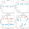 |
Fig. A.1. Relative differences between three different ipole image resolutions (162, 642, and 1962), for all Stokes parameters. In the case of Stokes 𝒰, we have shifted the curve 4 units higher for readability reasons. The bottom right plot shows the full light curves for Stokes 𝒬 and 𝒰, since fractional differences can be misleading for values close to zero. |
The second test we performed determined the relation of the first to the secondary image, and how in particular the latter is affected by the resolution. The results are shown in Fig. A.2, where it is clear that with a resolution of 16 × 16, it is really hard to capture the contribution of the secondary image to Stokes ℐ precisely, but at 64 × 64, the light curve resembles the higher resolution.
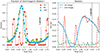 |
Fig. A.2. Comparison of emission from the first and the secondary image for different image resolutions. Left: Fraction of intensity contributed by the secondary image to the total Stokes I in a full period. The colors denote different image resolutions (162, 642, and 1962). Right: Absolute flux of the primary (solid line) and secondary (dashed line) image for the same three resolutions. |
Appendix B: Spin estimates
Although the spin estimates acquired in this work are simply a byproduct of our fitting algorithm and not the main focus of our analysis, we discuss them in some more detail.
In the first panel of Fig. B.1, we present what happens to our best-bet model if we keep all parameters the same and only change the spin to a* = 0. While the difference is not dramatic (the model still produces  ), it is certainly noticeable. To answer the question of what might cause this, we refer to panels 2 and 3, where we plot the light curves for the primary and secondary image separately. The middle panel clearly shows that the secondary image is necessary to produce the extreme similarity of our best-bet model with the data because the fit quality drops to
  . Another striking observation is that the difference between the models now is negligible. This most likely comes from the slight change in the period (affected by spin for a fixed orbital radius and Keplerianity parameter) from 92.5 to 89.5 min. This is further supported in the right panel of Fig. B.1, where the two light curves, corresponding to the secondary image alone, are shown. The differences are significant, more than 200% in relative terms and over 0.015 Jy in terms of the absolute flux density. This explains the spin preference, even though the spot is located so far way from the black hole. The dominant effect comes from the secondary image, which is formed by photons approaching the photon shell, which is located much closer to the black hole. A further analysis of the secondary image behavior and its dependence on the black hole spin necessitates a separate future work.
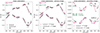 |
Fig. B.1. Difference in 𝒬, 𝒰 light curves from the best-bet model (nc_fb_nk), and the same model, but with the spin fixed to a* = 0 (nc_fb_nk_a0). Left: Full light curve. Middle: Primary image. Right: Secondary image. |
All Tables
𝒬sha, 𝒰sha values for all models obtained in the first fitting step, as well as the average values of 𝒬 and 𝒰 from the ALMA data.
All Figures
|
Fig. 1. Observed Sgr A* light curves for Stokes 𝒬 and 𝒰 from ALMA (W22). We only plot the points of the 35 time stamps that were used to infer the model parameters and not the 710 time stamps from the original light curve. |
| In the text | |
|
Fig. 2. Triangle and trace plots of the synthetic light-curve fitting. Top: Triangle plot, a combination of 1D and 2D marginalized posteriors, with the dashed lines denoting the median and 2σ or (90%) confidence levels (left and right). Similarly, the contours are for 90% (outer) and then 50% and 25% confidence levels. The truth is marked with red lines. Bottom: Trace plots showing the evolution of particles (and their marginal posterior distributions) in 1D projections, where lnX denotes the prior volume of the parameter space. The dots are color-coded with respect to their relative posterior mass, meaning that bright yellow values are present when convergence is achieved. |
| In the text | |
|
Fig. 3. Triangle plot and light curves for the Keplerian spot models without cooling (Kcoef = 1, Ccoef = 0). Top: Triangle plot of the posterior distributions for all parameters. The results for the two magnetic field polarities are shown in different colors, and their respected log(Evidence) values are reported in the label. Bottom: Best-fit model 𝒬 − 𝒰 light curves and 𝒬 − 𝒰 loops (color points) overplotted with ALMA observational data (gray points). The |
| In the text | |
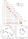 |
Fig. 4. Same as in Fig. 3, but for Keplerian models with cooling (Kcoef = 1, Ccoef ≠ 0). |
| In the text | |
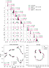 |
Fig. 5. Same as in Fig. 3, but for non-Keplerian models without cooling (Kcoef ≠ 1,Ccoef = 0). |
| In the text | |
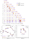 |
Fig. 6. Same as in Fig. 3, but for non-Keplerian models with cooling (Kcoef ≠ 1, Ccoef ≠ 0). |
| In the text | |
|
Fig. 7. Stokes ℐ, 𝒱 light curves for all models compared to the observational data from Wielgus et al. (2022a) and W22 (obs). The arrows represent a constant background component to facilitate comparison with the real data. |
| In the text | |
|
Fig. 8. Triangle plots for the background solution. The geometric parameters (i, a, PA), and Kcoef for nk cases were fixed at the values of the initial runs for the two Bfield orientations (color-coded) and without (left panels) and with cooling (right panels). |
| In the text | |
|
Fig. 9. Snapshot from the end of the light curve from our best-fitting model (nc_fb_nk), using 642 resolution, for Stokes ℐ, EVPA, fractional linear polarization (LP), and fractional circular polarization (CP). |
| In the text | |
|
Fig. A.1. Relative differences between three different ipole image resolutions (162, 642, and 1962), for all Stokes parameters. In the case of Stokes 𝒰, we have shifted the curve 4 units higher for readability reasons. The bottom right plot shows the full light curves for Stokes 𝒬 and 𝒰, since fractional differences can be misleading for values close to zero. |
| In the text | |
|
Fig. A.2. Comparison of emission from the first and the secondary image for different image resolutions. Left: Fraction of intensity contributed by the secondary image to the total Stokes I in a full period. The colors denote different image resolutions (162, 642, and 1962). Right: Absolute flux of the primary (solid line) and secondary (dashed line) image for the same three resolutions. |
| In the text | |
|
Fig. B.1. Difference in 𝒬, 𝒰 light curves from the best-bet model (nc_fb_nk), and the same model, but with the spin fixed to a* = 0 (nc_fb_nk_a0). Left: Full light curve. Middle: Primary image. Right: Secondary image. |
| In the text | |
Current usage metrics show cumulative count of Article Views (full-text article views including HTML views, PDF and ePub downloads, according to the available data) and Abstracts Views on Vision4Press platform.
Data correspond to usage on the plateform after 2015. The current usage metrics is available 48-96 hours after online publication and is updated daily on week days.
Initial download of the metrics may take a while.