| Issue |
A&A
Volume 691, November 2024
|
|
|---|---|---|
| Article Number | A327 | |
| Number of page(s) | 13 | |
| Section | Astrophysical processes | |
| DOI | https://doi.org/10.1051/0004-6361/202451884 | |
| Published online | 25 November 2024 | |
Hot spots around Sagittarius A*
Joint fits to astrometry and polarimetry
1
Department of Astrophysics/IMAPP, Radboud University, PO Box 9010 6500 GL Nijmegen, The Netherlands
2
Instituto de Astrofísica de Andalucía-CSIC, Glorieta de la Astronomía s/n, E-18008 Granada, Spain
3
Max-Planck-Institut für Radioastronomie, Auf dem Hügel 69, 53121 Bonn, Germany
⋆ Corresponding authors; a.yfantis@astro.ru.nl, maciek@wielgus.info
Received:
13
August
2024
Accepted:
10
October
2024
Context. Observations of Sagittarius A* (Sgr A*) in the near-infrared (NIR) show irregular flaring activity. Flares coincide with the astrometric rotation of the brightness centroid and with looping patterns in fractional linear polarization. These signatures can be explained with a model of a bright hot spot, transiently orbiting the black hole.
Aims. We extend the capabilities of the existing algorithms to perform parameter estimation and model comparison in the Bayesian framework using NIR observations from the GRAVITY instrument, and simultaneously fitting the astrometric and polarimetric data.
Methods. Using the numerical radiative transfer code ipole, we defined several geometric models describing a hot spot orbiting Sgr A*, threaded with a magnetic field, and emitting synchrotron radiation. We then explored the posterior space of our models with a nested sampling code dynesty. We used Bayesian evidence to make comparisons between the models.
Results. We have used 11 models to sharpen our understanding of the importance of various aspects of the orbital model, such as non-Keplerian motion, hot-spot size, and off-equatorial orbit. All considered models converge to realizations that fit the data well, but the equatorial super-Keplerian model is favoured by the currently available NIR dataset.
Conclusions. We have inferred an inclination of ∼155 deg, which corroborates previous estimates, a preferred period of ∼70 minutes, and an orbital radius of ∼12 gravitational radii with the orbital velocity of ∼1.3 times the Keplerian value. A hot spot with a diameter smaller than 5 gravitational radii is favoured. Black hole spin is not constrained well.
Key words: black hole physics / magnetic fields / polarization / methods: numerical / methods: statistical / Galaxy: center
© The Authors 2024
 Open Access article, published by EDP Sciences, under the terms of the Creative Commons Attribution License (https://creativecommons.org/licenses/by/4.0), which permits unrestricted use, distribution, and reproduction in any medium, provided the original work is properly cited.
This article is published in open access under the Subscribe-to-Open model. Subscribe to A&A to support open access publication.
1. Introduction
The supermassive black hole (SMBH) in our Galactic Centre, Sagittarius A* (Sgr A*), is a unique laboratory for studying dynamics near the black hole (BH) event horizon. With the Sgr A* mass of 4.3 × 10⁶ M⊙ (GRAVITY Collaboration 2022; Event Horizon Telescope Collaboration 2022a), the corresponding dynamical timescale at the innermost stable circular orbit (ISCO) is about 30 min assuming Schwarzschild space-time. This timescale sets our approximate expectations for the compact source variability, if it can be attributed to a physical orbiting component, rather than to a pattern motion (e.g. Matsumoto et al. 2020; Conroy et al. 2023).
Sgr A* exhibits frequent high energy outbursts, during which the near-infrared (NIR) flux density grows by 1–2 orders of magnitude (GRAVITY Collaboration 2020a). It has been proposed that the observed NIR flares correspond to an energized orbiting component – a hot spot (e.g. Broderick & Loeb 2006; Trippe et al. 2007; Hamaus et al. 2009; Tiede et al. 2020). Since 2018, the GRAVITY Collaboration has observed astrometric motion of the Sgr A* brightness centroid and polarimetric signatures associated with flares (GRAVITY Collaboration 2018, 2023) with the Very Large Telescope Interferometer (VLTI), supporting the hot-spot interpretation. Further observational support comes from the analysis of Atacama Large Millimeter/submillimeter Array (ALMA) polarimetric data, exhibiting similar observational features, associated with an X-ray flare (Wielgus et al. 2022a,b; Event Horizon Telescope Collaboration 2022b). A number of recent papers attempted to explain the detailed physics behind the formation of these polarimetric signatures of orbital motion (Gelles et al. 2021; Vos et al. 2022; Vincent et al. 2024) and to use the phenomenological hot-spot models to interpret NIR (GRAVITY Collaboration 2020b,c; Ball et al. 2021; Aimar et al. 2023) and millimetre (Wielgus et al. 2022b; Yfantis et al. 2024; Levis et al. 2024) data. Despite the variety of modelling setups and assumptions, all of these studies concluded a coherent clockwise orbital motion at a radius of roughly 10 M, on a low inclination near a face-on orbit (150 − 160 deg), with a vertical magnetic field component manifesting itself in the observations.
On the theoretical front, the hot-spot model phenomenology has been connected to the physics of magnetically arrested disk (MAD; Narayan et al. 2003) accretion systems, exhibiting flux eruption events resembling flaring activity of Sgr A* (Dexter et al. 2020; Scepi et al. 2022), and occasionally forming transiently orbiting flux tubes – large bubbles of electrons heated by reconnection and threaded with a predominantly vertical magnetic field (Porth et al. 2021; Ripperda et al. 2022). Numerical simulations show that such features may produce signatures consistent with the observations (Najafi-Ziyazi et al. 2024).
For this paper we further developed our Bayesian algorithm bipole1 (Yfantis et al. 2024, hereafter Y24), which was previously used for fitting the polarimetric millimetre observations of ALMA. We deployed bipole to simultaneously fit the polarimetric and astrometric NIR data of GRAVITY, presented in GRAVITY Collaboration (2023, hereafter G23). The analysis presented in G23 was based on fitting astrometric data, with constraints derived from polarimetry.
For our analysis we estimated the parameters of the hot-spot motion in order to compare them with the reported results from GRAVITY (G23) and ALMA (Wielgus et al. 2022b), as well as to discuss model selection in the Bayesian framework, using a statistically meaningful argument of the Bayesian evidence comparison. Our main findings are that the model constrains dynamical parameters of the hot-spot orbit, additionally showing preference for super-Keplerian orbital velocity and for a small hot-spot size. Black hole spin is not constrained well and the more complicated models, involving background emission or off-equatorial orbit, are not favoured.
2. Methods
In this section we describe the data, the model, and the fitting algorithm used to perform parameter estimation. The setup closely resembles the one developed in Y24 for the millimetre wavelength data analysis, including accounting for the finite light velocity (‘slow light’) and incorporating a complete model of the radiative transfer. Hence, in this paper we focus on presenting the differences between the specific applications to ALMA and to GRAVITY datasets.
2.1. Data
We utilized the data corresponding to the ensemble average of eight NIR flaring events (six with polarimetric and four with astrometric data available), observed by GRAVITY from 2018–2022 and first presented in G23 (see Fig. 1). Thus, following G23, we assume that separate events can be averaged together, that is, there exist well-defined mean parameters of the system, such as dynamical parameters of the hot-spot orbital motion. Furthermore, we assume that averaging between events helps to constrain these characteristic mean parameters by suppressing stochastic features of independent events. The data differ from ALMA observations (Wielgus et al. 2022b), analysed in Y24, in several ways. A much shorter observing wavelength (2.2 μm) implies a negligible impact of Faraday effects and synchrotron self-absorption. These effects presented a challenge for the millimetre data analysis (Wielgus et al. 2022b, 2024; Event Horizon Telescope Collaboration 2024). A shorter wavelength and higher energy of the emitting electrons also invalidate the assumption of a constant intrinsic radiative spectral power density of the orbiter as the NIR cooling timescale is generally expected to be shorter than the dynamical timescale. Hence, in order to avoid detailed modelling the internal physics of the source (e.g. Aimar et al. 2023), we worked with fractional polarization components (𝒬/ℐ and 𝒰/ℐ), which are robust against the changes of the intrinsic emission. What is more, the data cadence and error budgets differ significantly, as ALMA provides a much higher signal-to-noise ratio and cadence. On the other hand, GRAVITY data include astrometric information corresponding to the relative motion of the brightness centroid, which is simultaneous with the polarimetric variation, while ALMA provides no astrometric data.
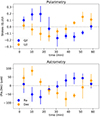 |
Fig. 1. Ensemble averaged dataset from G23. Top: Polarimetric data, fractional linear polarization components 𝒬/ℐ and 𝒰/ℐ as a function of time. Bottom: Astrometric data, brightness centroid position on the observer’s screen X (relative right ascension, Ra) and Y (relative declination, Dec) as a function of time. |
2.2. Model
We adopted the model used in Y24 to enable analysis of the NIR datasets. In NIR we expect the orbiting feature to dominate over the background, given a large change in brightness between the quiescent and flaring state (Do et al. 2019; GRAVITY Collaboration 2020a). This is in contrast to millimetre wavelengths, for which only a small change in brightness is present (e.g. Wielgus et al. 2022a). Hence, there is most likely no need to model a background accretion disk component for the NIR case. We tested this assumption with one of our hot-spot models discussed in Sect. 3.
On the other hand, the electron energy distribution (EED) plays a more important role in the NIR than at millimetre wavelengths, and it is most certainly non-thermal during the flaring state of the source. In bipole we assume a thermal relativistic EED. While no differences are expected for the astrometric data, the EED has an impact in the fractional polarization (Rybicki & Lightman 1979). The observed fractional polarization will additionally decrease in the partially incoherent magnetic field, which seems to be the case given the values observed by GRAVITY, peaking at about 25% (G23). Since this effect is difficult to be properly captured in a simple geometric model, we included an additional parameter LPfrac to scale the model fractional polarization with a constant number. Furthermore, the internal physics of the hot spot, which is probed only through fractional polarization, is not constrained well and degenerates between number density, temperature (or, more generally, EED), and the magnetic field strength for the synchrotron origin of the emission. For that reason we fixed the dimensionless electron temperature to a large value of Θe = 500, encouraging emission at the 2.2 μm wavelength. We additionally fixed the peak number density of the hot spot to ne = 107 cm−3, so the only estimated parameter related to the internal physics is the magnetic field strength B0, s. Given the nature of the data, it can essentially be considered to be a nuisance parameter, enforcing the idea that the synchrotron emission extends to the considered frequency.
The hot spot itself was modelled as a Gaussian blob with a radius (1 σ) of 3 M (M ≡rg = GM/c2, we used G = c = 1 units when it did not lead to ambiguities) and the Gaussian tail was suppressed at 1.5 σ. We assumed a clockwise direction for the orbital motion, which is strongly constrained by the astrometric data. The simulated hot spot travels as a rigid body on a circular orbit in the equatorial plane, with a constant orbital velocity equal to a fraction of the Keplerian orbital speed at the hot-spot centre, which was modelled with the Kcoef parameter. It affects the period of a circular orbit, which is given in Kerr space-time by
![$$ \begin{aligned} P=\frac{2\pi }{K_{\mathrm{coef}}}\frac{r_g}{c}\left[\left(\frac{r}{r_g}\right)^{1.5} + a_*\right], \end{aligned} $$](/articles/aa/full_html/2024/11/aa51884-24/aa51884-24-eq1.gif)
where r = rs is the distance of the spot from the BH centre, rg = GM/c2 is the gravitational radius, and a* = Jc/GM2 is the dimensionless BH spin. These aspects of the setup follow Vos et al. (2022) and Y24, and we assumed the magnetic field to be vertical in the comoving frame of the hot spot, similarly as in Y24 and consistent with the conclusions of GRAVITY Collaboration (2018), Wielgus et al. (2022b), and G23. This is also consistent with the theoretical expectations from magnetic reconnection in the equatorial current sheet (Porth et al. 2021; Ripperda et al. 2022). New developments include fitting astrometric data with the imaged hot-spot brightness centroid, fitting for the hot-spot size, joint model of a hot spot and a constant background component, and enabling circular off-equatorial orbits. Unlike in G23, our hot spot is not a Keplerian point source, we also did not neglect the impact of higher order images2, and we simultaneously fitted the astrometric and polarimetric observations.
2.3. Fitting procedure
We updated bipole in order to enable the simultaneous fitting of astrometric and polarimetric data. The software combines ipole, which is a ray-tracing code for the covariant general relativistic transport of polarized light in curved space-times developed in Mościbrodzka & Gammie (2018) with the nested sampling Bayesian tool dynesty, introduced by Speagle (2020) and further developed by Koposov et al. (2023).
The resolution of ray-traced images calculated by ipole was set to 64 × 64 pixels (see the discussion on the limitations of the resolution in Y24) and the dynesty sampling parameters were set to 800 live points with 100 extra live points for five batches, using the dynamical sampler introduced by Higson et al. (2019). The remaining hyper-parameters were identical with the setup of Y24, resulting in a single likelihood evaluation on a synthetic movie of an orbiting hot spot calculated in 0.5 second using a 24 cores machine3. The log-likelihood function ℒ was defined in a standard way as
![$$ \begin{aligned} \mathcal{L} (\boldsymbol{p}) = -\sum _j^S\frac{\left[S_j-\hat{S}_j(\boldsymbol{p})\right]^2}{2\sigma _{S,j}^2}\,, \end{aligned} $$](/articles/aa/full_html/2024/11/aa51884-24/aa51884-24-eq2.gif)
where p is the vector of the model parameters that are to be estimated, S represents the observed values of the four fitted quantities 𝒬 , 𝒰 , X, and Y, while  represents the predictions of the model. The uncertainties σS, j follow the values reported in G23. A list of all the fitted model parameters and their prior ranges is shown in Table 1.
Parameters and prior ranges used for the fitting.
3. Results
We fitted 11 variants of the orbiting hot-spot model to the dataset of G23 in order to understand the constraints posed by the NIR observations. The models and their performance are summarized in Table 2. We used the logarithm of the Bayesian evidence (marginal model likelihood) log(Z) as a statistically meaningful method to compare among models of different level of complication. At the level of uncertainties reported by G23, all considered variants produce good quality fits to the data, as indicated by the reduced effective (normalized by the number of data points minus the number of model parameters) χeff2 metric for the maximum likelihood estimators (MLEs), reported in Table 2. Our most successful models are the equatorial super-Keplerian ones without background emission. The orbital inclination is well constrained across the models to be around 155° ±5°, which is also consistent with constraints from G23, which were obtained with the Keplerian point source model of Gelles et al. (2021), as well as with ALMA constraints from Wielgus et al. (2022b) and Y24. Below we provide a description of the models and discuss constraints on other parameters. Quantitative information about the results of the fitting and associated uncertainties is given in Appendix A.
Hot-spot models used to fit Sgr A* GRAVITY data.
Evidence uncertainties. For the first test, we performed the fit of an orbiting hot spot on a Keplerian (circular time-like geodesic) orbit, using the two different polarities of the vertical magnetic field Bfield, models K_db and K_fb. The magnetic field polarity impacts the results only through Faraday effects, which should be negligible for NIR frequencies. As expected, two models find very similar MLE parameters. However, the estimated log evidence differs by 0.7. We used this result to calibrate the uncertainties of the evidence, concluding that in order to claim one model is preferable to another, we require a log-evidence difference of at least Δlog Z = 2.0. The models that we characterize as disfavoured have Δlog Z > 3.5 with respect to the best performing models. This corresponds to a Bayes factor of K > 33, indicating very strong preference in the model selection (Jeffreys 1998).
Orbital velocity and radius. We then compared the performance of super-Keplerian (supK_db) and sub-Keplerian (subK_db) models. There is some preference for super-Keplerian motion following the log-evidence argument (Δlog Z = 2.4, see Table 2); however, Keplerian, super-Keplerian, and sub-Keplerian MLEs all match the data well, as indicated in Fig. 2. In the case of the sub-Keplerian model, the ML estimator approaches the Keplerian limit, which is another indication that sub-Keplerian models are disfavoured. There are theoretical arguments for super-Keplerian, off-equatorial orbits, for example, by Ripperda et al. (2020), Matsumoto et al. (2020), and Lin et al. (2023). In particular, Aimar et al. (2023) discuss super-Keplerian motion of jet features tied to the equatorial plane at a smaller radius with magnetic forces. Preference was also given to super-Keplerianity in the case of equatorial orbit models by Antonopoulou & Nathanail (2024). Our analysis disfavours sub-Keplerian models, especially for typical MAD values, Kcoeff ∼ 0.5, thus encouraging these possibilities.
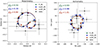 |
Fig. 2. Light curves from the ML estimators for models K_db, supK_db, and subK_db. The solid lines correspond to a max-likelihood (ML) estimator, which was recalculated at a higher image resolution (192 × 192). The χeff2 was calculated separately for polarimetry and astrometry. |
The quantity constrained well by the dataset is the period of the motion. Given the flexibility of non-Keplerian models there is a range of orbital velocities (scaled with Kcoeff) and orbital radii rs, that sustain the period to about 70 minutes. We make a conservative estimate of the orbital radius rs = 11 ± 2 M, which is consistent between the models. This value is also consistent with previous estimates, although slightly larger than that typically reported in the NIR of rs ≈ 9 M (GRAVITY Collaboration 2020b, G23).
Black hole spin. With the subsequent test, our aim was to see if the data constrain a deviation of the BH spin from a default assumption of Schwarzschild space-time (a* = 0). For that purpose we tested super- and sub-Keplerian models with the spin fixed to zero, supK_db_a0, and subK_db_a0, respectively. Fixing the spin results in only a very small decrease in the log-evidence, which is less than the assumed threshold for the model selection and less than the evidence estimation uncertainties. We conclude that the BH spin cannot be robustly inferred from the current dataset and its impact on the models is much less significant than that of the non-Keplerian orbital velocity. This is further confirmed by very broad and non-constraining BH spin posteriors in all other models as seen in the corner plots presented in Appendix A.
Spin axis position angle. The parameter PA, corresponding to the position angle of the BH spin on the observer’s screen appears to be well-constrained, much like the orbital inclination (see Table 2). The value we find, PA ∼130° ±20°, differs significantly from 180° reported in G23, but it is identical to the value reported in Ball et al. (2021), PA = 135°. On the other hand, for the ALMA dataset, Wielgus et al. (2022b) reported 57° (or 237°, given the model degeneracy) under the external Faraday screen model, which corresponds to 25° (or 205°) with the internal Faraday screen assumption and Y24 found reasonably consistent values under the internal Faraday screen assumption (see also Wielgus et al. 2024). Thus, we tested models with a PA fixed to 180° (supK_db_pa180 and subK_db_pa180). These models performed worse, and they can be disfavoured based on the log-evidence criterion. We conclude that the PA can be estimated based on this dataset, and that the value of 180° is disfavoured.
Hot-spot size. Our next test involved varying the size of the hot spot in the supK_db_ss variant of the model; this was done with the parameter ss that adjusts the 1 σ radius of the spot. By default, we used a large hot spot (ss = 3M) to allow for lower resolution of the reconstructed images and the computation time to be sped up. In order to model smaller hot spots, we increased the resolution from 64 × 64 to 192 × 192. We noticed only a marginal improvement of the log evidence for this more general model with respect to the supK_db model. Nonetheless, the marginalized posterior distribution indicates a preference for smaller hot-spot size. The results correspond to an upper limit on the hot-spot size at ss = 2.16 M (full width at half maximum of 5.09 M) at the 68% confidence level. This is a similar conclusion to the one given in GRAVITY Collaboration (2020b), where the hot-spot diameter was estimated to be smaller than 5 M. In our idealized geometric model, the change in hot-spot size manifests through detailed light curve properties, but the effect of depolarization from integrating over a large emission region is parametrized away with the LPfrac coefficient (see comments in Sect. 2.2). Nonetheless, we obtained consistent values of LPfrac = 0.2 (see Fig. A.5), indicating that the degree of depolarization is similar for a range of hot-spot sizes. This could be a consequence of an idealized geometric model, and the differences may be more pronounced for a realistic turbulent flow. Another argument favouring a smaller hot spot is related to shearing in a differential accretion flow, which we did not model here; for more details, readers can refer to GRAVITY Collaboration (2020b) and Tiede et al. (2020).
Accretion disk component. With the model supK_db_BG, we investigated a presence of another emission component, associated with the background accretion disk, which was invoked in G23 and other works. We modelled this component as an unpolarized feature with its brightness centroid located at the origin of the coordinate system. It affects both astrometric results (by reducing the width of the observed brightness centroid loop), and the polarimetric ones (by increasing the total flux density in the denominator of the fractional polarization). Adding a background component to a model results in a decrease in the log evidence by 2.9, which we interpret as the presence of a background emitter being discouraged by the data.
Off-equatorial orbit. For the final test, we considered a model supK_db_ofst, allowing for an off-equatorial, non-geodesic hot-spot orbit, at a fixed Boyer-Lindquist radius r and latitude θ, either in the background or in the foreground of the equatorial plane. This setup could model flux tubes or plasmoids in the jet’s sheath, both supported by pressure and magnetic forces (e.g. Ripperda et al. 2020). The offset results in an astrometric shift of the BH position by (Xoff, Yoff), which are additional fitted parameters, making this variant our most complicated one with a total of 11 degrees of freedom (Table 2). A reason to consider this generalization is related to the potential presence of a shift between the astrometric location of the Sgr A* centre of mass and the centre of the astrometric loops (GRAVITY Collaboration 2018), as well as hints of a super-Keplerian off-equatorial hot-spot motion (Matsumoto et al. 2020; Aimar et al. 2023). This model neither improves log evidence nor χeff2. Thus, our conclusion is that the available data do not support more general off-equatorial models.
4. Summary and conclusions
Very simple phenomenological models of an orbiting hot spot nicely explain the astrometric and polarimetric NIR observations of flaring Sgr A* obtained by VLTI/GRAVITY. Given the associated uncertainties, one overfits the data already with the basic Keplerian equatorial model. Nonetheless, the relative likelihood of the models can be studied, and constraints on different model parameters can be compared. We find that these models consistently constrain parameters of orbital radius, inclination, and the observed PA of the axis normal to the orbital plane (spin axis). The depolarization of the orbiting component is also constrained, and the preference for a smaller size of the emitting region is identified. We also show how BH spin is not constrained by the available dataset. Furthermore, super-Keplerian motion is favoured over sub-Keplerian. We show that data are consistent with one zone emission model (only the orbiting hot spot and no background emission) and with the near equatorial orbit model (±20°). More complicated models, such as the separate background component, are not justified by the constraining power of the currently available datasets.
There are excellent prospects for future observations of flaring Sgr A* to test, validate, and sharpen the orbital model. In the NIR, the upgraded GRAVITY instrument (GRAVITY+ Collaboration 2022) will provide improved observing sensitivity. Additionally, it is particularly interesting to study NIR flares with simultaneous (sub-)millimetre monitoring, which can be done with ALMA with full polarization, at an extremely high signal-to-noise ratio and time cadence. Simultaneous observations with very long baseline interferometric arrays could, in the near future, allow for the structure of the flaring source to be resolved in both time and space (Emami et al. 2023; Johnson et al. 2023). Such multiwavelength observations would not only yield a strong test of the hot-spot model, but they would also enable detailed studies of thermodynamics of the orbiting component to better understand the mechanism and energetics behind the phenomenon of flares. Development of dedicated data analysis pipelines, as the one presented in this paper, will be crucial to extract science from these more constraining future observations.
bipole (Bayesian ipole) refers to the combination of ipole (Mościbrodzka & Gammie 2018) with dynesty (Speagle 2020).
Acknowledgments
We thank F. Vincent, M. Bauböck, and D. Ribeiro for useful discussions. We also thank Paris Observatory in Meudon, where part of this research was conducted, for the hospitality. This publication is a part of the project Dutch Black Hole Consortium (with project number NWA 1292.19.202) of the research programme of the National Science Agenda which is financed by the Dutch Research Council (NWO). MM and AY acknowledge support from NWO, grant no. OCENW.KLEIN.113. MM also acknowledges support by the NWO Science Athena Award. AY thanks the “Summer School for Astrostatistics in Crete” for providing training on the statistical methods adopted in this work.
References
- Aimar, N., Dmytriiev, A., Vincent, F. H., et al. 2023, A&A, 672, A62 [NASA ADS] [CrossRef] [EDP Sciences] [Google Scholar]
- Antonopoulou, E., & Nathanail, A. 2024, A&A, 690, A240 [NASA ADS] [CrossRef] [EDP Sciences] [Google Scholar]
- Ball, D., Özel, F., Christian, P., Chan, C.-K., & Psaltis, D. 2021, ApJ, 917, 8 [NASA ADS] [CrossRef] [Google Scholar]
- Broderick, A. E., & Loeb, A. 2006, MNRAS, 367, 905 [Google Scholar]
- Conroy, N. S., Bauböck, M., Dhruv, V., et al. 2023, ApJ, 951, 46 [CrossRef] [Google Scholar]
- Dexter, J., Tchekhovskoy, A., Jiménez-Rosales, A., et al. 2020, MNRAS, 497, 4999 [Google Scholar]
- Do, T., Witzel, G., Gautam, A. K., et al. 2019, ApJ, 882, L27 [NASA ADS] [CrossRef] [Google Scholar]
- Event Horizon Telescope Collaboration (Akiyama, K., et al.) 2022a, ApJ, 930, L12 [NASA ADS] [CrossRef] [Google Scholar]
- Event Horizon Telescope Collaboration (Akiyama, K., et al.) 2022b, ApJ, 930, L13 [NASA ADS] [CrossRef] [Google Scholar]
- Event Horizon Telescope Collaboration (Akiyama, K., et al.) 2024, ApJ, 964, L26 [CrossRef] [Google Scholar]
- Emami, R., Tiede, P., Doeleman, S. S., et al. 2023, Galaxies, 11, 23 [NASA ADS] [CrossRef] [Google Scholar]
- Gelles, Z., Himwich, E., Johnson, M. D., & Palumbo, D. C. M. 2021, Phys. Rev. D, 104, 044060 [NASA ADS] [CrossRef] [Google Scholar]
- GRAVITY Collaboration (Abuter, R., et al.) 2018, A&A, 618, L10 [NASA ADS] [CrossRef] [EDP Sciences] [Google Scholar]
- GRAVITY Collaboration (Abuter, R., et al.) 2020a, A&A, 638, A2 [NASA ADS] [CrossRef] [EDP Sciences] [Google Scholar]
- GRAVITY Collaboration (Bauböck, M., et al.) 2020b, A&A, 635, A143 [CrossRef] [EDP Sciences] [Google Scholar]
- GRAVITY Collaboration (Jiménez-Rosales, A., et al.) 2020c, A&A, 643, A56 [CrossRef] [EDP Sciences] [Google Scholar]
- GRAVITY Collaboration (Abuter, R., et al.) 2022, A&A, 657, L12 [NASA ADS] [CrossRef] [Google Scholar]
- GRAVITY Collaboration (Abuter, R., et al.) 2023, A&A, 677, L10 [NASA ADS] [CrossRef] [EDP Sciences] [Google Scholar]
- GRAVITY+ Collaboration (Abuter, R., et al.) 2022, The Messenger, 189, 17 [NASA ADS] [Google Scholar]
- Hamaus, N., Paumard, T., Müller, T., et al. 2009, ApJ, 692, 902 [NASA ADS] [CrossRef] [Google Scholar]
- Higson, E., Handley, W., Hobson, M., & Lasenby, A. 2019, Statistics and Computing [Google Scholar]
- Jeffreys, H. 1998, The Theory of Probability, Oxford Classic Texts in the Physical Sciences (Oxford: OUP) [Google Scholar]
- Johnson, M. D., Akiyama, K., Blackburn, L., et al. 2023, Galaxies, 11, 61 [NASA ADS] [CrossRef] [Google Scholar]
- Koposov, S., Speagle, J., Barbary, K., et al. 2023, https://doi.org/10.5281/zenodo.7995596 [Google Scholar]
- Levis, A., Chael, A. A., Bouman, K. L., Wielgus, M., & Srinivasan, P. P. 2024, Nat. Astron., 8, 765 [NASA ADS] [CrossRef] [Google Scholar]
- Lin, X., Li, Y.-P., & Yuan, F. 2023, MNRAS, 520, 1271 [NASA ADS] [CrossRef] [Google Scholar]
- Matsumoto, T., Chan, C.-H., & Piran, T. 2020, MNRAS, 497, 2385 [NASA ADS] [CrossRef] [Google Scholar]
- Mościbrodzka, M., & Gammie, C. F. 2018, MNRAS, 475, 43 [CrossRef] [Google Scholar]
- Najafi-Ziyazi, M., Davelaar, J., Mizuno, Y., & Porth, O. 2024, MNRAS, 531, 3961 [NASA ADS] [CrossRef] [Google Scholar]
- Narayan, R., Igumenshchev, I. V., & Abramowicz, M. A. 2003, PASJ, 55, L69 [NASA ADS] [Google Scholar]
- Porth, O., Mizuno, Y., Younsi, Z., & Fromm, C. M. 2021, MNRAS, 502, 2023 [NASA ADS] [CrossRef] [Google Scholar]
- Ripperda, B., Bacchini, F., & Philippov, A. A. 2020, ApJ, 900, 100 [NASA ADS] [CrossRef] [Google Scholar]
- Ripperda, B., Liska, M., Chatterjee, K., et al. 2022, ApJ, 924, L32 [NASA ADS] [CrossRef] [Google Scholar]
- Rybicki, G. B., & Lightman, A. P. 1979, Radiative processes in astrophysics [Google Scholar]
- Scepi, N., Dexter, J., & Begelman, M. C. 2022, MNRAS, 511, 3536 [NASA ADS] [CrossRef] [Google Scholar]
- Speagle, J. S. 2020, MNRAS, 493, 3132 [Google Scholar]
- Tiede, P., Pu, H.-Y., Broderick, A. E., et al. 2020, ApJ, 892, 132 [NASA ADS] [CrossRef] [Google Scholar]
- Trippe, S., Paumard, T., Ott, T., et al. 2007, MNRAS, 375, 764 [NASA ADS] [CrossRef] [Google Scholar]
- Vincent, F. H., Wielgus, M., Aimar, N., Paumard, T., & Perrin, G. 2024, A&A, 684, A194 [NASA ADS] [CrossRef] [EDP Sciences] [Google Scholar]
- Vos, J., Mościbrodzka, M. A., & Wielgus, M. 2022, A&A, 668, A185 [NASA ADS] [CrossRef] [EDP Sciences] [Google Scholar]
- Wielgus, M., Marchili, N., Martí-Vidal, I., et al. 2022a, ApJ, 930, L19 [NASA ADS] [CrossRef] [Google Scholar]
- Wielgus, M., Moscibrodzka, M., Vos, J., et al. 2022b, A&A, 665, L6 [NASA ADS] [CrossRef] [EDP Sciences] [Google Scholar]
- Wielgus, M., Issaoun, S., Martí-Vidal, I., et al. 2024, A&A, 682, A97 [NASA ADS] [CrossRef] [EDP Sciences] [Google Scholar]
- Yfantis, A. I., Mościbrodzka, M. A., Wielgus, M., Vos, J. T., & Jimenez-Rosales, A. 2024, A&A, 685, A142 [NASA ADS] [CrossRef] [EDP Sciences] [Google Scholar]
Appendix A: Posterior distributions for the fitted models
We characterize the posterior distributions of our 11 models fitted to data with the following corner plots. Above the one-dimensional posteriors on the diagonal we provide the estimates of the fitted parameters as a median of the distribution with a 68% confidence interval (thin dashed lines in diagonal panels). We also present the maximum likelihood estimator (thick black lines in the corner plot) and its consistency with the data (below the corner plots). The presentation of the models follows the order from Table 2.
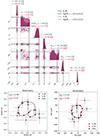 |
Fig. A.1. Top: Corner plot of the posterior distributions for all fitted parameters for the Keplerian orbital velocity models K_db and K_fb. The results for the two magnetic field polarities are shown in different colours, and their respected log-evidence values are reported in the legend. Bottom: Maximum likelihood estimators compared to the data. Points denote the fitting using observational timestamps, while lines are made in post-processing for visual aid. |
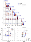 |
Fig. A.2. Same as Fig. A.1 but for models supK_db and subK_db, comparing sub-Keplerian and super-Keplerian setup. |
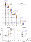 |
Fig. A.3. Same as Fig. A.1 but for models supK_db_a0 and subK_db_a0, testing for sensitivity to the BH spin. |
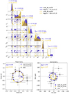 |
Fig. A.4. Same as Fig. A.1 but for models supK_db_pa180 and subK_db_180, testing for sensitivity to the observed PA of the spin axis. |
All Tables
All Figures
|
Fig. 1. Ensemble averaged dataset from G23. Top: Polarimetric data, fractional linear polarization components 𝒬/ℐ and 𝒰/ℐ as a function of time. Bottom: Astrometric data, brightness centroid position on the observer’s screen X (relative right ascension, Ra) and Y (relative declination, Dec) as a function of time. |
| In the text | |
|
Fig. 2. Light curves from the ML estimators for models K_db, supK_db, and subK_db. The solid lines correspond to a max-likelihood (ML) estimator, which was recalculated at a higher image resolution (192 × 192). The χeff2 was calculated separately for polarimetry and astrometry. |
| In the text | |
|
Fig. A.1. Top: Corner plot of the posterior distributions for all fitted parameters for the Keplerian orbital velocity models K_db and K_fb. The results for the two magnetic field polarities are shown in different colours, and their respected log-evidence values are reported in the legend. Bottom: Maximum likelihood estimators compared to the data. Points denote the fitting using observational timestamps, while lines are made in post-processing for visual aid. |
| In the text | |
|
Fig. A.2. Same as Fig. A.1 but for models supK_db and subK_db, comparing sub-Keplerian and super-Keplerian setup. |
| In the text | |
|
Fig. A.3. Same as Fig. A.1 but for models supK_db_a0 and subK_db_a0, testing for sensitivity to the BH spin. |
| In the text | |
|
Fig. A.4. Same as Fig. A.1 but for models supK_db_pa180 and subK_db_180, testing for sensitivity to the observed PA of the spin axis. |
| In the text | |
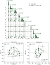 |
Fig. A.5. Same as in Fig. A.1 but for the model with variable hot-spot size supK_db_ss. |
| In the text | |
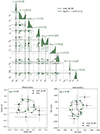 |
Fig. A.6. Same as Fig. A.1 but for the background component supK_db_BG model. |
| In the text | |
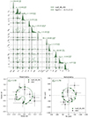 |
Fig. A.7. Same as Fig. A.1 but for the off-equatorial orbit model supK_db_ofst. |
| In the text | |
Current usage metrics show cumulative count of Article Views (full-text article views including HTML views, PDF and ePub downloads, according to the available data) and Abstracts Views on Vision4Press platform.
Data correspond to usage on the plateform after 2015. The current usage metrics is available 48-96 hours after online publication and is updated daily on week days.
Initial download of the metrics may take a while.